Interaction of a quantum well with squeezed light: Quantum statistical properties

Abstract

We investigate the quantum statistical properties of the light emitted by a quantum well interacting with squeezed light from a degenerate subthreshold optical parametric oscillator. We obtain analytical solutions for the pertinent quantum Langevin equations in the strong coupling and low excitation regimes. Using these solutions we calculate the intensity spectrum, autocorrelation function, quadrature squeezing for the fluorescent light. We show that the fluorescent light exhibits bunching and quadrature squeezing. We also show that the squeezed light leads to narrowing of the width of the spectrum of the fluorescent light.

I Introduction

Interaction of electromagnetic radiation with atoms has led to interesting quantum features such as antibunching and squeezing. In particular, interaction of two-level atoms with squeezed light has extensively been studied by many authors Gardiner86 ; Erenso02 ; Alebachew06 . These studies show that the squeezed light modifies the width of the spectrum of the incoherent light emitted by the atom. On the other hand, cavity QED in semiconductor systems has been the subject of interest in connection with its potential application in optoelectronic devices shiedls07 ; Baas04 ; Eleuch10 ; Eleuch08 ; Eleuch04 ; Giacobino02 . For example, such optical systems hold potential in realization of optical devices that exhibits exceptional properties such as monomode luminescence with high gain allowing the realization of thresholdless laser. The quantum properties of the light emitted by a quantum well embedded in a microcavity has been studied by several authors Karr04 ; Qatrtropani05 ; Eleuch08a . Unlike antibunching observed in atomic cavity QED, the fluorescent light emitted by the quantum well exhibits bunching Erenso03 ; Vyas00 . In the strong coupling regime–when the coupling frequency between the exciton and photon is larger than the relaxation frequencies of the medium and the cavity–the intensity spectrum of the exciton-cavity system has two well-resolved peaks representing two plaritons resonance Chen95 ; Wang97 . In the experimental setting, Weisbuch et al. Weisbuch92 demonstrated exciton-photon mode splitting in a semiconductor microcavity when the quantum well and the optical cavity are in resonance. Subsequent experiments on exciton-photon coupling confirmed normal mode splitting and oscillatory emission from exciton microcavities Pau95 ; Jacobson95 .

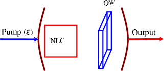
In this work, we study the effect of the squeezed light generated by a subthreshold degenerate parametric oscillator (OPO) on the squeezing and statistical properties of the fluorescent light emitted by a quantum well in a cavity. The system is outlined in Fig. 1. Degenerate OPO operating below threshold is a well-known source of squeezed light Lugiato83 ; Milburn83 . We explore the interaction between this light and a quantum well with a single exciton mode placed in the OPO cavity. Our analysis is restricted to the weak excitation regime where the density of excitons is small so that the interactions between an exciton and its neighbors can be neglected. Further, to gain insight into the physics we investigate the dynamics of the fluorescent light emitted by the quantum well in the strong coupling regime, which amounts to keeping the leading terms in the photon-exciton coupling constant $g$. We show that the fluorescent light exhibits bunching and quadrature squeezing. The former is due to the fact that two or more excitons in the quantum well can be excited by absorbing cavity photons. This implies there is a finite probability that two photons can be emitted simultaneously. We also show that the squeezed light leads to narrowing of the width of the spectrum of the fluorescent light.

We obtain the solution of the quantum Langevin equation for a cavity coupled to vacuum reservoir. The resulting solution, in the strong coupling limit, is used to calculate the intensity, spectrum, second order correlation function and quadrature squeezing of the fluorescent light.

II Hamiltonian and equations of evolution

We consider a system composed of a semiconductor quantum well and a degenerate parametric oscillator operating below threshold. In a degenerate parametric oscillator, a pump photon of frequency $2\omega_{0}$ is downconverted into a pair of identical sinal photons of frequency $\omega_{0}$. The signal photons are highly correlated and this correlation is responsible to the reduction of noise below the vacuum level. Such a system produces a maximum intracavity squeezing of 50$\%$. In a quantum well, the electromagnetic field can excite an electron from the filled valance band to the conduction band thereby creating a hole in the valance band. The electron-hole system possesses bound states which is also called exciton states analogous to the hydrogenic states or more precisely to the positronium bound states. We assume that the density of the excitons is small so that exciton-exciton interaction is negligible. The Hamiltonian describing the parametric process and interaction between exciton and cavity mode in the rotating wave approximation and at resonance is given by

$$H=\frac{i\varepsilon}{2}(a^{\dagger 2}-a^{2})+ig(a^{\dagger}b-ab^{\dagger})+H_{\text{loss}}.$$ (1)

Here $a$ and $b$, considered as boson operators, are the annihilation operators for the cavity and exciton modes, respectively; $g$ is the exciton cavity mode coupling; $H_{\text{loss}}$ is the Hamiltonian associated with the dissipation of the cavity and exciton modes by vacuum reservoir modes.

Figure 1: Schematic representation of a driven cavity containing a nonlinear crystal (NLC) and a quantum well (QW).

We assume here that the amplitude of the field $\varepsilon$ that drives the cavity is real and constant. The quantum Langevin equations of the system taking into account the cavity dissipation $\kappa$ and the exciton spontaneous emission $\gamma$ can be written as

$$\frac{da}{dt}=-\frac{\kappa}{2}a+\varepsilon a^{\dagger}+gb+F_{c}(t),$$ (2)

$$\frac{db}{dt}=-\frac{\gamma}{2}b-ga+F_{e}(t),$$ (3)

where $F_{c}$ and $F_{e}$ are the Langevin noise operators for the cavity and exciton modes, respectively. Both noise operators have zero mean, i.e., $\langle F_{c}\rangle=\langle F_{e}\rangle=0$. For a cavity mode damped by a vacuum reservoir, the noise operator satisfy the following correlations:

$$\left\langle F_{c}(t)F_{c}^{\dagger}(t^{\prime})\right\rangle=\kappa\delta(t-t^{\prime}),$$ (4)

$$\left\langle F_{c}^{\dagger}(t)F_{c}(t^{\prime})\right\rangle=\left\langle F_{c}(t)F_{c}(t^{\prime})\right\rangle=\left\langle F_{c}^{\dagger}(t)F_{c}^{\dagger}(t^{\prime})\right\rangle=0.$$ (5)

The exciton noise operators satisfy the following correlations:

$$\left\langle F_{e}(t)F_{e}^{\dagger}(t^{\prime})\right\rangle=\gamma\delta(t-t^{\prime}),$$ (6)

$$\left\langle F_{e}^{\dagger}(t)F_{e}(t^{\prime})\right\rangle=\left\langle F_{e}(t)F_{e}(t^{\prime})\right\rangle=\left\langle F_{e}^{\dagger}(t)F_{e}^{\dagger}(t^{\prime})\right\rangle=0.$$ (7)

III Photon statistics

In this section we analyze the photon statistics of he fluorescent light by calculating intensity, intensity spectrum and second order correlation function in the strong coupling regime. The solution of Eqs. (2) and (3) is rigorously derived in the Appendix. In the paper paper is devoted to the dynamics of the system in the strong coupling regime. To this end, imposing the strong coupling limit ($g\gg\kappa,\gamma$), which amounts to keeping only the leading terms in $g$, one obtains from Eqs. (41) and (46) that $\Delta=\Lambda=4ig$. As a result, the solution given by Eqs. (A) and (A) reduce to

$$a(t) =\lambda_{1}^{(+)}(t)a(0)+\lambda_{2}^{(+)}(t)a^{\dagger}(0)+\lambda_{3}(t)b(0)+\lambda_{4}(t)b^{\dagger}(0)$$

$$+\int_{0}^{t}dt^{\prime}~{}~{}\big{[}\lambda_{1}^{(+)}(t-t^{\prime})F_{c}(t^{\prime})+\lambda_{2}^{(+)}(t-t^{\prime})F_{c}^{\dagger}(t^{\prime})\big{]}$$

$$+\int_{0}^{t}dt^{\prime}~{}~{}\big{[}\lambda_{3}(t-t^{\prime})F_{e}(t^{\prime})+\lambda_{4}(t-t^{\prime})F_{e}^{\dagger}(t^{\prime})\big{]},$$ (8)

$$b(t) =\lambda_{1}^{(-)}(t)b(0)+\lambda_{2}^{(-)}(t)b^{\dagger}(0)-\lambda_{3}(t)a(0)-\lambda_{4}(t)a^{\dagger}(0)$$

$$-\int_{0}^{t}dt^{\prime}~{}~{}\big{[}\lambda_{3}(t-t^{\prime})F_{c}(t^{\prime})+\lambda_{4}(t-t^{\prime})F_{c}^{\dagger}(t^{\prime})\big{]}$$

$$+\int_{0}^{t}dt^{\prime}~{}~{}\big{[}\lambda_{1}^{(-)}(t-t^{\prime})F_{e}(t^{\prime})+\lambda_{2}^{(-)}(t-t^{\prime})F_{e}^{\dagger}(t^{\prime})\big{]},$$ (9)

where

$$\lambda_{1}^{(\pm)}(t) =\Big{[}\Big{(}\cos(gt)\pm\frac{\gamma-\kappa}{4g}\sin(gt)\Big{)}\cosh(\varepsilon t/2)$$

$$\pm\frac{\varepsilon}{2g}\sin(gt)\sinh(\varepsilon t/2)\Big{]}e^{-(\kappa+\gamma)t/4},$$ (10)

$$\lambda_{2}^{(\pm)}(t) =\Big{[}\Big{(}\cos(gt)\pm\frac{\gamma-\kappa}{4g}\sin(gt)\Big{)}\sinh(\varepsilon t/2)$$

$$\pm\frac{\varepsilon}{2g}\sin(gt)\cosh(\varepsilon t/2)\Big{]}e^{-(\kappa+\gamma)t/4},$$ (11)

$$\lambda_{3}(t)=\sin(gt)\cosh(\varepsilon t/2)e^{-(\kappa+\gamma)t/4},$$ (12)

$$\lambda_{4}(t)=\sin(gt)\sinh(\varepsilon t/2)e^{-(\kappa+\gamma)t/4}.$$ (13)

All quantities of interest which describe the dynamics of the system can fully be analyzed using these solutions.

III.1 Intensity of fluorescent light

The dynamical behavior of the intensity of light emitted by a single quantum well in GaAs microcavity has been measured experimentally Jacobson95 . We here seek to study the dynamical behavior of the light emitted by a single quantum well interacting with squeezed light. The intensity of the fluorescent light is proportional to the mean number of excitons in the system. Using Eq. (III) and the properties of the noise forces, we readily obtain

$$\langle b^{\dagger}b\rangle =\frac{2\varepsilon^{2}}{(\kappa+\gamma)^{2}-4\varepsilon^{2}}+\frac{1}{2}\bigg{[}\big{(}1+\bar{n}_{e}+\bar{n}_{e}\cos(2gt)$$

$$+\frac{\kappa-\gamma}{4g}(1+2\bar{n}_{e})\sin(2gt)\big{)}\cosh(\varepsilon t)$$

$$-\frac{1}{4g}[\kappa-\gamma+2\varepsilon(1+2\bar{n}_{e})\sin(gt)]\sinh(\varepsilon t)$$

$$-(\kappa+\gamma)\frac{2\varepsilon\sinh(\varepsilon t)+(\kappa+\gamma)\cosh(\varepsilon t)}{(\kappa+\gamma)^{2}-4\varepsilon^{2}}$$

$$+\frac{\gamma-\kappa}{2g}\text{sinh}^{2}(\varepsilon t/2)\text{sin}(2gt)\bigg{]}e^{-(\kappa+\gamma)t/2},$$ (14)

where $\bar{n}_{e}$ is the mean exciton number in the cavity at initial time. We assumed that the cavity mode is initially in vacuum state. It is easy to see that in the steady state the mean exciton number reduces to

$$\langle b^{\dagger}(t)b(t)\rangle_{ss}=\frac{2\varepsilon^{2}}{(\kappa+\gamma)^{2}-4\varepsilon^{2}},$$ (15)

which is a contribution to intensity of the fluorescent light due to the optical parametric oscillator.

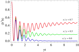
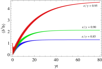
Figure 2: Plots of the fluorescent intensity [Eq. (III.1)] vs scaled time $\gamma t$ for $\gamma=\kappa$, $g/\gamma=5$, $\bar{n}_{e}=1$ and for different values of $\varepsilon/\gamma$.

Figure 3: Plots of the fluorescent intensity [Eq. (III.1)] near threshold vs scaled time $\gamma t$ for $\kappa/\gamma=1$, $g/\gamma=5$, $\bar{n}_{e}=1$ and for different values of $\varepsilon/\gamma$.

In Fig. 2, we plot the intensity as a function of scaled time $\gamma t$ for different values of the scaled pump field amplitude $\varepsilon/\gamma$. In this figure we have assumed that the cavity in initially prepared in such a way that it contains one exciton($\bar{n}_{e}=1$) but no photon. For simplicity we have taken the cavity and exciton decay rate to be the same, i.e., $\kappa=\gamma$. This figure shows the effect of the parametric oscillator on the intensity fluorescent light. It is not hard to see that the intensity oscillates with frequency equal to the coupling constant $g$, which is a signature of exchange of energy between the cavity and exciton modes. Moreover, the amplitude of the oscillations depends on the amplitude of the pump field, $\varepsilon$, which represents the optical parametric oscillator in our system. The stronger the pump field and the higher the amplitude of oscillation and the longer it takes to reach the steady state value of the intensity.

It worth emphasizing that since optical parametric oscillator is operating below threshold, the parameter $\varepsilon$ is constrained by the inequality $\kappa+\gamma>2\varepsilon$. We thus interpret $\kappa+\gamma=2\varepsilon$ as threshold condition for the parametric process. In the vicinity of the threshold the mean exciton number increases rapidly and exceeds unity as illustrated in Fig. 3. This shows that even though there is one exciton in the cavity initially, there is a finite probability for the squeezed light in the cavity to excite two or more excitons in the quantum well. This has an interesting effect on the photon statistics of the fluorescent light as discussed in Section C.

III.2 Intensity spectrum

We next proceed to calculate the power spectrum of the fluorescent light. The power spectrum of the fluorescent light can be expressed in terms of the bosonic operator as

$$S(\omega)=\frac{1}{\pi}\text{Re}\int_{0}^{\infty}d\tau~{}e^{i\omega\tau}\frac{\langle b^{\dagger}(t)b(t+\tau)\rangle_{ss}}{\langle b^{\dagger}(t)b(t)\rangle_{ss}}.$$ (16)

In the strong coupling regime the correlation function that appears in the integrand of the power spectrum in the steady state has the form

$$\frac{\langle b^{\dagger}(t)b(t+\tau)\rangle_{ss}}{\langle b^{\dagger}(t)b(t)\rangle_{ss}} =\Big{[}\frac{\gamma((\kappa+\gamma)^{2}-4\varepsilon^{2})}{4g(\kappa+\gamma)\varepsilon}\sin(g\tau)\sinh(\varepsilon\tau/2)$$

$$+\frac{\cos(gt)}{2\varepsilon}\big{(}2\varepsilon\cosh(\varepsilon\tau/2)$$

$$+(\kappa+\gamma)\sinh(\varepsilon\tau/2)\big{)}\Big{]}e^{-(\kappa+\gamma)\tau/4}.$$ (17)

Substituting this result in Eq. (16) and keeping the leading order in $g$, we obtain the power spectrum of the fluorescent light to be

$$S(\omega) =\frac{\gamma_{+}\gamma_{-}}{2\pi\varepsilon g(\kappa+\gamma)}\Big{[}\frac{g\kappa+3g\gamma-2\gamma\omega}{\gamma_{-}^{2}+(g-\omega)^{2}}-\frac{g\kappa+3g\gamma-2\gamma\omega}{\gamma_{+}^{2}+(g-\omega)^{2}}$$

$$+\frac{g\kappa+3g\gamma+2\gamma\omega}{\gamma_{-}^{2}+(g+\omega)^{2}}-\frac{g\kappa+3g\gamma+2\gamma\omega}{\gamma_{+}^{2}+(g+\omega)^{2}}\Big{]},$$ (18)

where $\gamma_{\pm}=(\gamma+\kappa\pm 2\varepsilon)/4$ are the half widths of the Lorentzians centered at $\omega=\pm g$. We immediately see that the width of the power spectrum depends on the amplitude of the pump field.

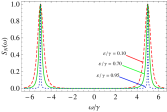
Figure 4: Plots the normalized intensity spectrum of the fluorescent light [$S_{N}(\omega)=S(\omega)/S(g)$] vs scaled frequency $\omega/\gamma$ for $\kappa/\gamma=1$, $g/\gamma=5$, $\bar{n}_{e}=1$, and for different values of $\varepsilon/\gamma$.

We observe that the maximum of the power spectrum occurs when the frequency equal to the coupling constant ($g$). In order of explore the effect of the squeezed light on the width of the spectrum it is convenient to plot the the power spectrum normalized by its maximum value, i.e., $S_{N}(\omega)=S(\omega)/S(g)$. In Fig. 4, we plot the normalized spectrum as a function of $\omega/\gamma$ for different values of the pump amplitude ($\varepsilon$). As clearly indicated in the figure, the the higher the amplitude of the pump field (the degree of squeezing), the narrower the width has become. It is also worth noting that the narrowing of the width is more pronounced close to the threshold, i.e., when the squeezing approaches to its maximum value. This is in contrary to the result obtained when the quantum well is coupled to a squeezed vacuum reservoir, where the spectrum is independent of the squeeze parameter Erenso03 .

We further note that the spectrum has two peaks symmetrically located at $\pm g$. This is the result of the strong coupling approximation ($g\gg\kappa,\gamma$). Both peaks have the same width which depends on the exciton and cavity modes decay rates and the amplitude of the pump field.

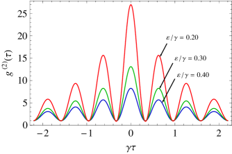
III.3 Autocorrelation function

5 We now turn our attention to the calculation of autocorrelation function, which is proportional to the probability of detecting one photon at $t+\tau$ given that another photon was detected at earlier time t. Quantum mechanically autocorrelation is defined by

$$g^{(2)}\left(\tau\right)=\frac{\left\langle b^{\dagger}(t)b^{\dagger}(t+\tau)b(t+\tau)b(t)\right\rangle}{\left\langle b^{\dagger}(t)b(t)\right\rangle^{2}}.$$ (19)

Using the Gaussian properties of the noise forces Walls94 , the autocorrelation function in the steady state can be put in a simpler form

$$g^{(2)}(\tau)=1+\frac{|\langle b^{\dagger}(t)b^{\dagger}(t+\tau)\rangle_{ss}|^{2}}{\langle b^{\dagger}(t)b(t)\rangle^{2}_{ss}}+\frac{|\langle b^{\dagger}(t)b(t+\tau)\rangle_{ss}|^{2}}{\langle b^{\dagger}(t)b(t)\rangle^{2}_{ss}}.$$ (20)

In order to find a closed form analytical expression for the autocorrelation function, one has to determine the two time correlation functions that appear in Eq. (19). This can be done using the solution (III) along with the correlation properties of the noise forces. After algebraic manipulations, we obtain the final expression of the autocorrelation function to be

$$g^{(2)}(\tau)=1+e^{-\frac{1}{2}(\kappa+\gamma)\tau}\cos(g\tau)\left[\mu_{1}\sin(g\tau)+\mu_{2}\cos(g\tau)\right],$$ (21)

where

$$\mu_{1}=\frac{\gamma((\kappa+\gamma)^{2}-4\varepsilon^{2})}{4g(\kappa+\gamma)\varepsilon^{2}}\left[(\kappa+\gamma)\cosh(\varepsilon\tau)+2\varepsilon\sinh(\varepsilon\tau)\right],$$

$$\mu_{2}=\frac{((\kappa+\gamma)^{2}+4\varepsilon^{2})\cosh(\varepsilon\tau)+4(\kappa+\gamma)\varepsilon\sinh(\varepsilon\tau)}{4\varepsilon^{2}}.$$

Expression (21) is valid only in the strong coupling regime ($g\gg\kappa,\gamma$).

The behavior of $g^{(2)}(\tau)$ as a function of the pump amplitude ($\varepsilon$) and for constant $g$ is illustrated in Fig. 5. This figure shows that the correlation function oscillates at frequency equals to $g$. The amplitude of this oscillations decreases fast when we increase the value of $\varepsilon$. The autocorrelation function at $\tau=0$ has the form $g^{(2)}(0)=2+(\kappa+\gamma)^{2}/4\varepsilon^{2}>1$ indicating the phenomenon of photon bunching. Here the underlying physics can be explained in terms of the mean exciton number (see Fig. 3). In that figure we have showed that, even though we start of one exciton initially, there is finite probability of exciting two or more excitons in the quantum well by the squeezed light. This allows the possibility of emission of two photon at a time which leads to of phenomenon of bunching in the fluorescent light.

Figure 5: Autocorrelation function versus normalized time $\gamma\tau$ for $g/\gamma=5$, $\kappa/\gamma=1$, $\bar{n}_{e}=1$, and for different value of pump amplitude $\varepsilon/\gamma$.

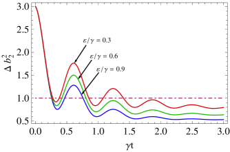
IV Quadrature squeezing

The squeezing properties of the fluorescent light can be analyzed by calculating the variances of the quadrature operators. The variances of the quadrature operators for the fluorescent light are given by

$$\Delta b_{1}^{2}=1+2\langle b^{\dagger}b\rangle+\langle b^{2}\rangle+\langle b^{\dagger 2}\rangle,$$ (22)

$$\Delta b_{2}^{2}=1+2\langle b^{\dagger}b\rangle-(\langle b^{2}\rangle+\langle b^{\dagger 2}\rangle),$$ (23)

where $b_{1}=b^{\dagger}+b$ and $b_{2}=i(b^{\dagger}-b)$. These quadrature operators satisfy the commutation relation $[b_{1},b_{2}]=2i$. On the basis of these definitions the fluorescent light is said to be in a squeezed state if either $\Delta b_{1}^{2}<1$ or $\Delta b_{2}^{2}<1$. In deriving $\eqref{Q1}$ and $\eqref{Q2}$ we have used $\langle b(t)\rangle=0$, which can easily be verified using $\eqref{A19eq}$. Applying Eq. (III) and the properties of the noise operators the variances turn out to be

$$\Delta b_{1}^{2}=1 +\frac{2\varepsilon}{k+\gamma-2\varepsilon}+e^{-(k+\gamma-2\varepsilon)t/2}A_{-}(t)$$

$$+e^{-(k+\gamma-\varepsilon)t/2}B_{-}(t),$$ (24)

$$\Delta b_{2}^{2}=1 -\frac{2\varepsilon}{k+\gamma+2\varepsilon}+e^{-(k+\gamma+2\varepsilon)t/2}A_{+}(t)$$

$$+e^{-(k+\gamma+\varepsilon)t/2}B_{+}(t),$$ (25)

in which

$$A_{\pm}(t) =1+\bar{n}_{e}+\bar{n}_{e}\cos(2gt)$$

$$\Big{[}\frac{\gamma-\kappa}{4g}e^{\pm\varepsilon t}+\frac{\kappa-\gamma\pm 2\varepsilon}{4g}(1+2\bar{n}_{e})\Big{]}\sin(2gt),$$

$$B_{\pm}(t)=-\frac{(\kappa+\gamma)e^{\pm\varepsilon t/2}}{\kappa+\gamma\pm 2\varepsilon}\pm\frac{\kappa-\gamma}{2g}\sinh(\varepsilon t/2)\sin(2gt).$$

It is straightforward to see that the variances reduce in the steady state to

$$\Delta b_{1}^{2} =1+\frac{2\varepsilon}{k+\gamma-2\varepsilon},$$ (26)

$$\Delta b_{2}^{2} =1-\frac{2\varepsilon}{k+\gamma+2\varepsilon}.$$ (27)

Expressions (26) and (27) represent the quadrature variance of a parametric oscillator operating below threshold. At threshold $\kappa+\gamma=2\varepsilon$, the squeezing becomes $50\%$ which is the maximum squeezing that can be obtained from subthreshold parametric oscillator Milburn83 . It is then not difficult to see that the squeezing occurs in the $b_{2}$ quadrature.

In Fig. 6, the time evolution of the variance of the $b_{2}$ quadrature, (IV), is plotted versus scaled time $\gamma t$. The variance in this quadrature oscillates with frequency equal to twice the Rabi frequency. The amplitude of oscillation damps out at longer time and eventually become flat at steady state. Moreover, it is interesting to note that the fluorescent light is not squeezed at initial moment however, it starts to exhibit transient squeezing before it becomes unsqueezed again. The more the exciton interacts with the squeezed light, the stronger the squeezing becomes. As a result of this we observe squeezed fluorescent light in longer periods which ultimately approaches to the $50\%$ maximum squeezing limit observed in parametric oscillator. The reduction of fluctuations noted in the fluorescent light is due to the interaction between the long-lived squeezed photons in the cavity and excitons in the quantum well. As can be seen from Fig. 6, the degree of squeezing of the fluorescent light depends on the amplitude of the pump field.

Figure 6: Plots of the quadrature variance [Eq. (IV)] vs scaled time $\gamma t$ for $g/\gamma=5$, $\kappa=\gamma$, $\bar{n}_{e}=1$ and for the different values of the pump field amplitude $\varepsilon/\gamma$.

V Conclusion

The quantum statistical properties of the fluorescent light emitted by exciton in a quantum well interacting with squeezed light is presented. Analytical solutions for the pertinent quantum Langevin equations are rigorously derived. These solutions, in the strong coupling limit in which the exciton-cavity mode coupling is much greater than the cavity as well as exciton spontaneous decay rates $(g\gg\kappa,\gamma)$ are used to study the dynamical behavior of the generated light. We find that the squeezed light enhances the mean photon number and narrows the width of the intensity spectrum of the fluorescent light. Further, the fluorescent light shows normal-mode splitting, which is a signature of strong coupling. We note that unlike atomic cavity QED where the fluorescent light exhibits antibunching, the fluorescent light in the present system rather exhibits bunching. The manifestation of bunching is attributed to the possibility of exciting two or more excitons in the quantum well which in turn leads a finite probability of emission of two photons simultaneously.

Appendix A Solution for the quantum Langevin equations

In this appendix we derive the solution of the following quantum Lagevin equations:

$$\frac{da}{dt}=-\frac{\kappa}{2}a+\varepsilon a^{\dagger}+gb+F_{c}(t),$$ (28)

$$\frac{db}{dt}=-\frac{\gamma}{2}b-ga+F_{e}(t).$$ (29)

In order to solve these equations it is more convenient to introduce new variable defined by

$$a_{\pm}=a^{\dagger}\pm a~{}~{}~{}~{}~{}~{}~{}~{}~{}b_{\pm}=b^{\dagger}\pm b.$$ (30)

With the help of Eqs. (28) and (29) and their complex adjoint we obtain

$$\frac{d}{dt}a_{+} = -\frac{1}{2}(\kappa-2\varepsilon)a_{+}+gb_{+}+F_{+}$$ (31)

$$\frac{d}{dt}b_{+} = -\frac{\gamma}{2}b_{+}-ga_{+}+G_{+}$$ (32)

$$\frac{d}{dt}a_{-} = -\frac{1}{2}(\kappa+2\varepsilon)a_{-}+gb_{-}+F_{-}$$ (33)

$$\frac{d}{dt}b_{-} = -\frac{\gamma}{2}b_{-}-ga_{-}+G_{-},$$ (34)

where $F_{\pm}=F_{c}^{\dagger}\pm F_{c}$ and $G_{\pm}=F_{e}^{\dagger}\pm F_{e}$. Note that Eqs. (31) and (32) are decoupled from (33) and (34). These coupled equations can be solved using the method of Laplace transform.

The Laplace transform of Eqs. (31) and (32) gives

$$A(s) =\frac{4g}{\chi}G(s)+\frac{2(2s+\gamma)}{\chi}F(s)$$

$$+\frac{1}{\chi}\big{[}4gb_{+}(0)+2(2s+\gamma)a_{+}(0)\big{]}$$ (35)

$$B(s) =\frac{2}{\chi}(\kappa+2s-2\varepsilon)G(s)-\frac{4g}{\chi}F(s)$$

$$+\frac{1}{\chi}\big{[}-4ga_{+}(0)+2(\kappa+2s-2\varepsilon)b_{+}(0)\big{]},$$ (36)

where $\chi=4g^{2}+(2s+\gamma)(\kappa+2s-2\varepsilon)$ and $A(s)=\mathcal{L}(a_{+}),B(s)=\mathcal{L}(b_{+}),G(s)=\mathcal{L}(G_{+})$ and $F(s)=\mathcal{L}(F_{+})$ with $\mathcal{L}$ denoting Laplace transform. The inverse Laplace transform of Eqs. (A) and (A) yields

$$a_{+}(t) =a_{+}(0)f_{+}(t)+b_{+}(0)f_{2}(t)+\int_{0}^{t}f_{+}(t-t^{\prime})F_{+}(t^{\prime})dt^{\prime}$$

$$+\int_{0}^{t}f_{2}(t-t^{\prime})G_{+}(t^{\prime})dt^{\prime}$$ (37)

$$b_{+}(t) =b_{+}(0)f_{-}(t)-a_{+}(0)f_{2}(t)+\int_{0}^{t}f_{-}(t-t^{\prime})G_{+}(t^{\prime})dt^{\prime}$$

$$-\int_{0}^{t}f_{2}(t-t^{\prime})F_{+}(t^{\prime})dt^{\prime},$$ (38)

where

$$f_{\pm}(t)=\left[\cosh(\Delta t/4)\pm\frac{\gamma-\kappa+2\varepsilon}{\Delta}\sinh(\Delta t/4)\right]e^{-\gamma_{-}t}$$ (39)

$$f_{2}(t)=\frac{4g}{\Delta}\sinh(\Delta t/4)e^{-\gamma_{-}t}.$$ (40)

$$\Delta=\sqrt{-16g^{2}+(\gamma-\kappa+2\varepsilon)^{2}},~{}~{}\gamma_{-}=\frac{1}{4}(\kappa+\gamma-2\varepsilon)$$ (41)

Note that the solution of the coupled equations (33) and (34) can easily be obtained by replacing $\varepsilon$ by $-\varepsilon$, $F_{+}$ by $F_{-}$, and $G_{+}$ by $G_{-}$ in the solution of Eqs. (31) and (32). We thus have

$$a_{-}(t) =a_{-}(0)h_{+}(t)+b_{-}(0)h_{2}(t)+\int_{0}^{t}h_{+}(t-t^{\prime})F_{-}(t^{\prime})dt^{\prime}$$

$$+\int_{0}^{t}h_{2}(t-t^{\prime})G_{-}(t^{\prime})dt^{\prime}$$ (42)

$$b_{-}(t) =b_{-}(0)h_{-}(t)-a_{-}(0)h_{2}(t)+\int_{0}^{t}h_{-}(t-t^{\prime})G_{-}(t^{\prime})dt^{\prime}$$

$$-\int_{0}^{t}h_{2}(t-t^{\prime})F_{-}(t^{\prime})dt^{\prime},$$ (43)

where

$$h_{\pm}(t)=\left[\cosh(\Lambda t/4)\pm\frac{\gamma-\kappa-2\varepsilon}{\Lambda}\sinh(\Lambda t/4)\right]e^{-\gamma_{+}t}$$ (44)

$$h_{2}(t)=\frac{4g}{\Lambda}\sinh(\Lambda t/4)e^{-\gamma_{+}t}.$$ (45)

$$\Lambda=\sqrt{-16g^{2}+(\gamma-\kappa-2\varepsilon)^{2}},~{}~{}\gamma_{+}=\frac{1}{4}(\kappa+\gamma+2\varepsilon)$$ (46)

Applying the inversion formula $a=(a_{+}-a_{-})/2$ and $b=(b_{+}-b_{-})/2$ the solution for $a(t)$ and $b(t)$ turn out to be

$$a(t) =\eta_{1}^{(+)}(t)a(0)+\eta_{2}^{(+)}(t)a^{\dagger}(0)+\eta_{3}^{(+)}(t)b(0)+\eta_{3}^{(-)}(t)b^{\dagger}(0)$$

$$+\int_{0}^{t}dt^{\prime}~{}~{}\big{[}\eta_{1}^{(+)}(t-t^{\prime})F_{c}(t^{\prime})+\eta_{2}^{(+)}(t-t^{\prime})F_{c}^{\dagger}(t^{\prime})\big{]}$$

$$+\int_{0}^{t}dt^{\prime}~{}~{}\big{[}\eta_{3}^{(+)}(t-t^{\prime})F_{e}(t^{\prime})+\eta_{3}^{(-)}(t-t^{\prime})F_{e}^{\dagger}(t^{\prime})\big{]},$$ (47)

$$b(t) =\eta_{1}^{(-)}(t)b(0)+\eta_{2}^{(-)}(t)b^{\dagger}(0)-\eta_{3}^{(+)}(t)a(0)-\eta_{3}^{(-)}(t)a^{\dagger}(0)$$

$$-\int_{0}^{t}dt^{\prime}~{}~{}\big{[}\eta_{3}^{(+)}(t-t^{\prime})F_{c}(t^{\prime})+\eta_{3}^{(-)}(t-t^{\prime})F_{c}^{\dagger}(t^{\prime})\big{]}$$

$$+\int_{0}^{t}dt^{\prime}~{}~{}\big{[}\eta_{1}^{(-)}(t-t^{\prime})F_{e}(t^{\prime})+\eta_{2}^{(-)}(t-t^{\prime})F_{e}^{\dagger}(t^{\prime})\big{]},$$ (48)

where

$$\eta_{1}^{(\pm)}(t) =\frac{1}{2}\Big{(}\cosh(\Delta t/4)\pm\frac{\gamma-\kappa+2\varepsilon}{\Delta}\sinh(\Delta t/4)\Big{)}e^{-\gamma_{-}t}$$

$$+\frac{1}{2}\Big{(}\cosh(\Lambda t/4)\pm\frac{\gamma-\kappa-2\varepsilon}{\Lambda}\sinh(\Lambda t/4)\Big{)}e^{-\gamma_{+}t}$$ (49)

$$\eta_{2}^{(\pm)}(t) =\frac{1}{2}\Big{(}\cosh(\Delta t/4)\pm\frac{\gamma-\kappa+2\varepsilon}{\Delta}\sinh(\Delta t/4)\Big{)}e^{-\gamma_{-}t}$$

$$-\frac{1}{2}\Big{(}\cosh(\Lambda t/4)\pm\frac{\gamma-\kappa-2\varepsilon}{\Lambda}\sinh(\Lambda t/4)\Big{)}e^{-\gamma_{+}t}$$ (50)

$$\eta_{3}^{(\pm)}(t)=\frac{2g}{\Delta}\sinh(\Delta t/4)e^{-\gamma_{-}t}\pm\frac{2g}{\Lambda}\sinh(\Lambda t/4)e^{-\gamma_{+}t}.$$ (51)

References

(1) C. W. Gardiner, Phys. Rev. Lett. 56, 1917 (1986).
(2) D. Erenso and R. Vyas, Phys. Rev. A 65, 063808 (2002).
(3) E. Alebachew and K. Fessaha, Opt. Comm. 271, 154
(2006); E. Alebachew, J. Mod. Opt. 55, 1159 (2008).
(4) A. J. Shields, Nature Photonics 1, 215 (2007).
(5) A. Baas, J. Ph. Karr, H. Eleuch, and E. Giacobino, Phys. Rev. A 69, 023809 (2004).
(6) H. Eleuch and N. Rachid, Eur. Phys. J. D 57, 259
(2010)
(7) H. Eleuch, J. Phys. B 41, 055502 (2008).
(8)H. Eleuch and R. Bennaceur, J. Opt. B 6, 189 (2004)
(9) E. Giacobino, J.Ph. Karrr, G. Messin, H. Eleuch, C.R. Physique 3, 41
(2002).
(10) J. Ph. Karr, A. Baas, R. Houdré and E. Giacobino Phys. Rev. A 69, 031802 (2004).
(11) A. Quattropani and P. Schwendimann, Phys. Status Solidi
242, 2302 (2005).
(12) H. Eleuch, Eur. Phys. J. D 49, 391
(2008); H. Eleuch, Eur. Phys. J. D 48, 139 (2008).
(13) D. Erenso, R. Vyas and S. Singh, Phys. Rev A
67,013818 (2003).
(14) R. Vyas and S. Singh, J. Opt. Soc. Am. B 7, 634 (2000).
(15) Y. Chen, A. Tredicucci and F. Bassani, Phys. Rev. B 52, 1800 (1995).
(16) H. Wang, Y. Chough, S. E. Palmer, and H. J. Carmichael, Opt. Express 1, 370 (1997).
(17) C. Weisbuch, M. Nishioka, A. Ishikawa, and Y. Arakawa,
Phys. Rev. Lett. 69, 3314 (1992).
(18) S. Pau, G. Björk, J. Jacobson, H. Cao, and Y. Yamamoto, Phys.
Rev. B 51, 14 437 (1995); H. Cao, J. Jacobson, et
al., Appl. Phys. Lett. 66, 1107 (1995).
(19) J. Jacobson, S. Pau, H. Cao, G. Björk,
and Y. Yamamoto, Phys. Rev. A 51, 2542 (1995).
(20) L. A. Lugiato and G. Strini, Opt. Comm. 41, 67 (1982).
(21) G. J. Milburn and D. F. Walls, Phys. Rev. A 27, 392
(1983).
(22) D. F. Walls and G. J. Milburn, Quantum Optics (Springer-Verlag, Berlin, 1994).