Complex dynamics in learning complicated games

Abstract

Game theory is the standard tool used to model strategic interactions in evolutionary biology and social science. Traditional game theory studies the equilibria of simple games. But is traditional game theory applicable if the game is complicated, and if not, what is? We investigate this question here, defining a complicated game as one with many possible moves, and therefore many possible payoffs conditional on those moves. We investigate two-person games in which the players learn based on experience. By generating games at random we show that under some circumstances the strategies of the two players converge to fixed points, but under others they follow limit cycles or chaotic attractors. The dimension of the chaotic attractors can be very high, implying that the dynamics of the strategies are effectively random. In the chaotic regime the payoffs fluctuate intermittently, showing bursts of rapid change punctuated by periods of quiescence, similar to what is observed in fluid turbulence and financial markets. Our results suggest that such intermittency is a highly generic phenomenon, and that there is a large parameter regime for which complicated strategic interactions generate inherently unpredictable behavior that is best described in the language of dynamical systems theory.

Traditional game theory usually gives a good understanding for simple games with a few players, or with only a few possible moves, characterizing the solutions in terms of their equilibria vonneumann ; nash . The applicability of this approach is not clear when the game becomes more complicated, for example due to more players or a larger strategy space, which can cause an explosion in the number of possible equilibria opper ; opper2 ; berg ; berg2 . This is further complicated if the players are not rational and must learn their strategies ho ; camerer ; camerer1 ; fudenberg ; young . In a few special cases it has been observed that the strategies display complex dynamics and fail to converge to equilibrium solutions sato ; skyrms ; hommes . Are such games special, or is this typical behavior? More generally, under what circumstances should we expect that games become so hard to learn that their dynamics fail to converge? What kind of behavior should we expect and how should we characterize the solutions?

As an example of what we mean compare the games of tic-tac-toe and chess. Tic-tac-toe is a simple game with only $765$ possible positions and $26,830$ distinct sequences of moves. Young children easily discover the Nash equilibrium, which results in a draw, at which point the game becomes uninteresting. In contrast, chess is a complicated game with roughly $10^{47}$ possible positions and $10^{123}$ possible sequences of moves; despite a huge effort, the Nash equilibrium (corresponding to an ideal game) remains unknown. Equilibrium concepts of game theory are not useful in describing complicated games such as chess or go (which has an even larger game tree with roughly $10^{360}$ possible sequences of moves). An example that is even closer to what we have in mind here is investing in financial markets, which is a non-zero sum game where players can choose between thousands of assets and a rich set of possible strategies.

Here we show that if the players use a standard approach to learning, for complicated games there is a large parameter regime in which one should expect complex dynamics. By this we mean that the players never converge to a fixed strategy. Instead their strategies continually vary as each player responds to past conditions and attempts to do better than the other players. The trajectories in the strategy space display high-dimensional chaos, suggesting that for most intents and purposes the behavior is essentially random, and the future evolution is inherently unpredictable.

I Model

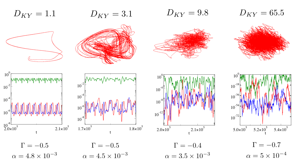
Figure 1: An illustration of complex learning dynamics, depicted in terms of trajectories of the strategy ${\bf x}^{\mu}(t)$ for different parameters ($\beta=0.01$). In (a) the attractor is a limit cycle, whereas (b-d) are chaotic attractors of increasingly high dimension. There are $N=50$ possible moves; the upper panel shows an arbitrary three-dimensional projection of each attractor in the $98$-dimensional phase space, and lower panels show the strategy as a function of time for the corresponding three coordinates. For clarity we use logarithmic scale. As the dimension of the attractor increases, so does the range of $x^{\mu}_{i}$. For the highest dimensional case a given move has occasional bursts where it is highly probable, and long periods where it is extremely improbable (as low as $10^{-72}$).

To address the questions raised above we study two-player games. For convenience call the two players Alice and Bob. At each time step $t$ player $\mu\in\mbox{\{Alice = A, Bob = B\}}$ chooses between one of $N$ possible moves, picking the $i^{th}$ move with frequency $x_{i}^{\mu}(t)$, where $i=1,\ldots,N$. The frequency vector ${\bf x}^{\mu}(t)=(x_{1}^{\mu},\dots,x_{N}^{\mu})$ is the strategy of player $\mu$. If Alice plays $i$ and Bob plays $j$, Alice receives receives payoff $\Pi_{ij}^{A}$ and Bob receives payoff $\Pi_{ji}^{B}$.

We assume that the players learn their strategies ${\bf x}^{\mu}$ via a form of reinforcement learning called experience weighted attraction. This has been extensively studied by experimental economists who have shown that it provides a reasonable approximation for how real people learn in games ho ; camerer1 ; camerer . Actions that have proved to be successful in the past are played more frequently and moves that have been less successful are played less frequently. To be more specific, the probability of a given move is

$$x_{i}^{\mu}(t)=\frac{e^{\beta Q_{i}^{\mu}(t)}}{\sum_{k}e^{\beta Q_{k}^{\mu}(t)}},$$ (1)

where $Q_{i}^{\mu}$ is called the attraction for player $i$ to strategy $\mu$. In the special case of experience weighted attraction that we use here, Alice’s attractions are updated according to

$$Q_{i}^{A}(t+1)=(1-\alpha)Q_{i}^{A}(t)+\sum_{j}\Pi_{ij}^{A}x_{j}^{B}$$ (2)

and similarly for Bob with $A$ and $B$ interchanged.

The dynamics for updating the strategies ${\bf x}^{\mu}$ of the two players are completely deterministic. This approximates the situation in which the players vary their strategies slowly in comparison to the timescale on which they play the game.

The key parameters that characterize the learning strategy are $\alpha$ and $\beta$. The parameter $\beta$ is called the intensity of choice; when $\beta$ is large a small historical advantage for a given move causes that move to be very probable, and when $\beta=0$ all moves are equally likely. The parameter $\alpha$ specifies the memory in the learning; when $\alpha$ = 1 there is no memory of previous learning steps, and when $\alpha=0$ all learning steps are remembered and are given equal weight, regardless of how far in the past. The case $\alpha=0$ corresponds to the much-studied replicator dynamics used to describe evolutionary processes in population biology sato2 ; nowak ; sigmund .

We choose games at random by drawing the elements of the payoff matrices $\Pi_{ij}^{\mu}$ from a normal distribution may ; opper ; opper2 ; berg ; berg2 . The mean and the covariance are chosen so that $E[\Pi_{ij}^{\mu}]=0$, $E[(\Pi^{\mu}_{ij})^{2}]=1/N$, and $E[\Pi_{ij}^{A}\Pi_{ji}^{B}]=\Gamma/N$, where $E[x]$ denotes the average of $x$. The variable $\Gamma$ is a crucial parameter which measures the deviation from a zero-sum game. When $\Gamma=-1$ the game is zero sum, i.e. the amount Alice wins is equal to the amount Bob loses, whereas when $\Gamma=0$ their payoffs are uncorrelated.

II Results

We simulate randomly constructed games with $N=50$ possible moves, corresponding to a $98$ dimensional state space (there are two $50$ dimensional strategy vectors and two probability constraints). The behavior observed depends on the parameters. In some cases we see stable learning dynamics, in which the strategies ${\bf x}^{\mu}$ of both players converge on a fixed point. For a large section of the parameter space, however, the strategies converge to a more complicated orbit, either a limit cycle or a chaotic attractor. We characterize the local stability properties of the attractors by numerically computing the Lyapunov exponents $\lambda_{i}$, $i=1,\ldots,2N-2$, which quantify the rate of expansion or contraction of nearby points in the state space. The Lyapunov exponents also determine the Lyapunov dimension $D$, which measures the number of degrees of freedom of the motion on the attractor.

We give several examples of the observed learning dynamics at different parameter values in Fig. 1. These include a limit cycle and chaotic attractors of varying dimensionality. There can also be long transients in which the trajectory follows a complicated orbit for a long time and then suddenly collapses into a fixed point. In general the behavior observed depends on the random draws of the payoff matrices $\Pi_{ij}^{\mu}$, but as we move away from the stability boundary, for a given set of parameters we observe fairly consistent behavior .

Simulating games at many different parameter values reveals the stability diagram given in Fig. 2. Roughly speaking we find that the dynamics are stable f1 when $\Gamma\approx-1$ (zero sum games) and $\alpha$ is large (short memory), i.e. in the lower right of the diagram, and unstable when $\Gamma\approx 0$ (uncorrelated payoffs) and $\alpha$ is small (long memory), i.e. in the upper left. Interestingly, for reasons that we do not understand the highest dimensional behavior is observed when the payoffs are moderately anti-correlated ($\Gamma\approx-0.6$) and when players have long-memory ($\alpha\approx 0$).

In order to make the problem analytically tractable we have made specific choices in the parameters for experience weighted attraction (EWA). Comparison with behavioral experiments modeled with EWA as reported in ho shows that the particular form we are using here is roughly within the range observed in real experiments. Values for memory-loss parameters and intensity of choice reported from experiments suggest that real-world decision making may well operate near or in the chaotic phase (see Supplementary Information). Most experimental data is limited to low-dimensional games however, whereas here we study games with a large number of possible moves. A good example where high dimensional chaotic behavior is likely is in financial markets, where there are a huge number of possible moves and learning times are measured in years. High dimensional chaotic behavior can be effectively indistinguishable from noise.

A good approximation of the boundary between the stable and unstable regions of the parameter space can be computed analytically using techniques from statistical physics. We use path-integral methods from the theory of disordered systems dedominicis ; opper to compute the stability in the limit of infinite payoff matrices, $N\to\infty$. We do this in a continuous-time limit where, for fixed $\Gamma$, stability then depends only on the ratio $\alpha/\beta$ (see Supplementary Information).

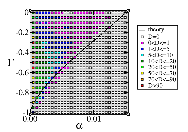
Figure 2: Stability diagram showing where stable vs. chaotic learning is likely ($\beta=0.01$). The solid line is the stability boundary estimated using path-integral methods. The coloured squares are from simulations of the learning dynamics and represent the typical dimension of the attractor (averaged over $10$ or more independent payoff matrices per data point).

We have simulated games for various values of $N$. If $D>0$ at small $N$, the dimension $D$ tends to increase with $N$. At this stage we have been unable to tell whether $D$ reaches a finite limit or grows without bound as $N\to\infty$.

An interesting property of this system is the time dependence of the received payoffs. As shown in Fig. 3, when the dynamics are chaotic the total payoff to all the players varies, with intermittent bursts of large fluctuations punctuated by relative quiescence. This is observed, although to varying degrees, throughout the chaotic part of the parameter space. There is a strong resemblance to the clustered volatility observed in financial markets, which in turn resembles the intermittency of fluid turbulence ghashghaie ; hommes . We also observe heavy tails in the distribution of the fluctuations, as described in more detail in the Supplementary Information. This suggests that these properties, which have received a great deal of attention in studies of financial markets, may occur simply because they are generic properties of complicated games f2 .

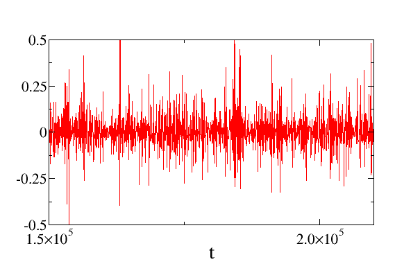
Figure 3: Chaotic dynamics display clustered volatility. We plot the difference of payoffs on successive time steps for case (c) in Fig. 1. The amplitude of the fluctuations increases with the dimension of the attractor.

III Why is dimensionality relevant?

The dimensionality $D$ is relevant to this problem because high dimensionality suggests that failure to converge to a fixed point is independent of the learning algorithm, i.e. the game is intrinsically hard to learn. The fact that the equilibria of a game are unlearnable with any particular learning algorithm, such as reinforcement learning, does not imply that learning is not possible with some other learning algorithm. For example, if the learning dynamics settles into a limit cycle or a low dimensional attractor, a careful observer could collect data and make better predictions about the other player using the method of analogues lorenz , or refinements based on local approximation farmer . If the dimension of the chaotic attractor is too high, however, the curse of dimensionality makes this impossible with any reasonable amount of data farmer . This suggests that there exists no learning algorithm that can provide an improvement when learning must occur inductively based on past data. The observation of high-dimensional dynamics here leads us to conjecture that there are some games that are inherently unlearnable, in the sense that any learning algorithms will inevitably result in high-dimensional chaotic learning dynamics (See also Sato et al. sato ).

Our work here makes it possible to predict a priori the qualitative properties of the learning dynamics of any given complicated two player game under reinforcement learning. This is because the payoff matrix of any given game is a possible draw from an ensemble of random games. One can make a good estimate of the stability properties of the learning dynamics by locating the game and the learning parameters in the stability diagram of Fig. 2. We have shown that a key property of a game is its “zero-sumness”, characterized by $\Gamma$. Games become harder to learn (in the sense that the strategies do not converge) when they are non-zero-sum, particularly if the players use learning algorithms with long memory. This analysis can potentially be extended to multiplayer games, games on networks, alternative learning algorithms, etc.

Our results suggest that under many circumstances it is more useful to abandon the tools of classic game theory in favor of those of dynamical systems. It also suggests that many behaviors that have attracted considerable interest, such as clustered volatility in financial markets, may simply be specific examples of a highly generic phenomenon, and should be expected to occur in a wide variety of different situations.

Appendix A Experience weighted attraction learning

A.1 General definitions for multi-player games

We here briefly describe the experience weighted attraction learning (EWA) model put forward in camerer ; camerer1 ; camerer2 . Consider a game played by $p$ players, who each choose from a set of $N$ actions (pure strategies) at each time step. In the EWA model the probability for player $\mu\in\{1,\dots,p\}$ to choose action $i\in\{1,\dots,N\}$ at time $t$ is

$$x^{\mu}_{i}(t)=\frac{e^{\beta Q^{\mu}_{i}(t)}}{\sum_{k}e^{\beta Q^{\mu}_{k}(t)}},$$ (3)

where the $\{Q_{i}^{\mu}\}$ are referred to as attractions or propensities. The basic idea is that $Q^{\mu}_{i}(t)$ gives the “attraction” of player $\mu$ to action $i$ at time $t$, based on how successful strategy $i$ has been in the past. The model parameter $\beta\geq 0$ is called the intensity of choice. For $\beta=0$ players pick actions with equal probability (i.e. they play completely at random), and for $\beta\to\infty$ each player’s choice is deterministic, i.e. that player will always choose the same action for given values of $Q_{i}^{\mu}$, namely the action with the highest attraction.

The update rule for the attractions $\{Q^{\mu}_{i}\}$ in the EWA model reads camerer ; camerer1 ; camerer2

$$Q^{\mu}_{i}(t+1)=\frac{\phi{\cal N}(t)Q^{\mu}_{i}(t)+[\delta+(1-\delta)I(i,s_{\mu}(t)]\Pi^{\mu}(i,\bm{s}_{-\mu}(t))}{{\cal N}(t)},$$ (4)

where the quantity ${\cal N}(t)$ is updated according to

$${\cal N}(t+1)=\phi(1-\kappa){\cal N}(t)+1,$$ (5)

see camerer1 . The notation is explained below:

• We write $s_{\mu}(t)\in\{1,\dots,N\}$ for the action player $\mu$ takes at time step $t$ in a given realization of the dynamics. The notation $-\mu$ labels all players other than $\mu$, i.e. $-\mu$ is the set $\{1,\dots,p\}\backslash\{\mu\}$. The notation $\bm{s}_{-\mu}(t)$ indicates the set of actions that the opponents of player $\mu$ took in a given round. Thus $\bm{s}_{-\mu}\in\{1,\dots,N\}^{p-1}$ is a $(p-1)$-component vector, each component of which is one of the possible actions.

• For a given $\bm{s}_{-\mu}(t)\in\{1,\dots,N\}^{p-1}$ the quantity $\Pi^{\mu}(i,\bm{s}_{-\mu}(t))$ is a payoff matrix element, and indicates the payoff player $\mu$ receives when playing pure strategy $i$ and facing the actions $\bm{s}_{-\mu}(t)$ of the other agents at time $t$.

• The variable $\cal{N}$ indicates a weight factor. An initial condition needs to be specified, which is then updated according to relation (5). When $\phi(1-\kappa)=1$, this is just the number of times the game has been played. In this case, since $\cal{N}$ cancels in the first term in the numerator on the RHS of Eq. (4), and since it divides the second term, as time goes on the influence of the updates becomes smaller and smaller, i.e. past moves have more weight than recent moves and the behavior becomes “set”.

• The notation $I(\cdot,\cdot)$ stands for the indicator function (also called the Kronecker delta), i.e. $I(a,b)=1$ if $a=b$ and $I(a,b)=0$ otherwise.

• The parameter $\delta$ specifies the relative weighting given to strategies that are played vs. those that are not played. In the case of $\delta=1$ players update all attractions $Q^{\mu}_{i}$ in every round, irrespective of what actions they actually took. The choice $\delta=0$ corresponds to a case where only the scores of strategies that are actually used in a given round are updated after that round.

• The parameter $\kappa$ interpolates between average reinforcement learning ($\kappa=0$) and cumulative reinforcement learning ($\kappa=1$), see camerer ; camerer1 ; camerer2 ; we have ${\cal N}(t)=1$ for all $t$ if $\kappa=1$, the attractions $Q_{i}^{\mu}$ then represent the cumulative outcome of all past play (depending on the choice of $\phi$ potentially discounted over time), for $\kappa=0$ the normalisation factor ${\cal N}(t)$ grows with time.

• The parameter $\phi$ specifies the weight of outcomes of play in the distant past relative to more recent iterations. If $\kappa=1$ and $\phi=1$ all past experience carries equal weight, no matter how much time has elapsed, for $\phi=0$ only the most recent round affects the players’ future decisions. Intermediate values of $\phi$ correspond to exponential discounting.

A.2 The specific case that we study here

There are many parameters within the formalism of experience weighted attraction, and it is beyond the scope of this paper to investigate all of the possible cases. We thus restrict ourselves to a particular case that is both analytically tractable and reasonably close to how real people play.

We first assume that Eq. (5) reaches a fixed point $\cal{N}^{*}$ in the long-run. Letting ${\cal{N}}(t+1)={\cal{N}}(t)={\cal N}^{*}$ gives

$${\cal N}^{*}=\frac{1}{1-\phi(1-\kappa)}.$$ (6)

The update rule then simplifies to

$$Q^{\mu}_{i}(t+1)=\phi Q^{\mu}_{i}(t)+(1-\phi(1-\kappa))[\delta+(1-\delta)I(i,\bm{s}_{\mu}(t)]\Pi^{\mu}(i,\bm{s}_{-\mu}(t)).$$ (7)

We will focus here on the case $\delta=1$, i.e. all strategy scores are updated in every iteration. Then we have

$$Q^{\mu}_{i}(t+1)=\phi Q^{\mu}_{i}(t)+(1-\phi(1-\kappa))\Pi^{\mu}(i,\bm{s}_{-\mu}(t)).$$ (8)

Focusing on cumulative re-inforcement learning camerer ; camerer1 ; camerer2 , i.e. the case $\kappa=1$, and replacing $\phi\rightarrow 1-\alpha$ for later convenience, we have

$$Q^{\mu}_{i}(t+1)=(1-\alpha)Q^{\mu}_{i}(t)+\Pi^{\mu}(i,\bm{s}_{-\mu}(t)).$$ (9)

Eq. (9) is the learning rule used in sato ; sato2 . The parameter $\alpha$ describes memory loss. For $\alpha=0$ past payoffs are not discounted, and the memory of players covers the full history of play. For $0<\alpha<1$ past payoffs are taken into account with exponentially decreasing weights.

To summarise, the learning model we investigate is defined by Eq. (3) together with Eq. (9):

• Eq. (3) specifies how a given player $\mu\in\{1,\dots,p\}$ translates his or her set of attractions $Q^{\mu}_{i}$, $i\in\{1,\dots,N\}$, into a mixed strategy $(x_{1}^{\mu},\dots,x_{N}^{\mu})$. He or she will choose action $\mu\in\{1,\dots,N\}$ with the probabilities defined by Eq. (3).

• Eq. (9) specifies how the attractions are updated from time step $t$ to $t+1$ once all players have chosen their actions in time step $t$.

The correspondence with the EWA model of camerer1 can be summarized as follows:

model of Camerer et al. $$\leftrightarrow$$ notation in present work

$$P_{\mu}^{i}~{}~{}~{}~{} \leftrightarrow ~{}~{}~{}~{}x^{\mu}_{i},$$

$$A_{\mu}^{i}~{}~{}~{}~{} \leftrightarrow ~{}~{}~{}~{}Q^{\mu}_{i},$$

$$\phi~{}~{}~{}~{} \leftrightarrow ~{}~{}~{}~{}1-\alpha.$$ (10)

A.3 Relation to experimental data

Parameters of the EWA learning model were fit to real-world data in camerer2 , see in particular Table 4. This table shows that there is substantial variation in the parameters that provide a best fit to the data across different games. While we have chosen parameters that were tractable for the theoretical calculations that follow, comparison to their experimental results indicates that these values are fairly reasonable. For example, they find values of the parameter $\kappa$ in the range $0.15$-$0.99$; we fix $\kappa=1$. The model parameter $\delta$ obtained from experimental data varies from $\delta=0$ to $\delta=0.94$, suggesting that there is no clear conclusion on whether or not players use forgone payoffs in their adaptation; we fix $\delta=1$, i.e. the propensities of all strategies are updated at every step.

The most interesting model parameters from the point of view of our analysis are the memory-loss parameter $\alpha$ and the intensity of choice $\beta$. For a fixed game, these parameters largely determine whether or not one should expect convergence or chaotic motion. More precisely the ratio $\alpha/\beta$ is the crucial indicator for the onset of chaos, as explained above. Pooled data from camerer2 suggests a ratio of $\alpha/\beta\approx 0.03$ (but again with considerable variation across games). Depending on the character of the game (zero-sum or not) this can position such experiments inside the chaotic phase, see Fig. 5. It is important to keep in mind, however, that the games used in the experiments of camerer2 are low-dimensional, in the sense that each player has the choice only between a small number of moves. Care needs to be taken when extrapolating results for high-dimensional random games to these cases. Nonetheless, if one assumes that parameters would not dramatically change in moving from simple games to complicated games, then the data and model fitting of camerer1 , taken together with our results, suggests that real-world learning in non-zero sum games may well operate in or near the chaotic phase.

A.4 Adiabatic limit and deterministic learning

The update of Eq. (9) is intrinsically stochastic, as the $(p-1)$-component action vector $\bm{s}_{-\mu}(t)$ at time $t$ is drawn according to the mixed strategy profiles of the $p-1$ opponents player $\mu$ is facing. More precisely, player $\mu$ will face a specific realization of the actions $\bm{s}_{-\mu}=(s_{1},\dots,s_{\mu-1},s_{\mu+1},\dots,s_{p})\in\{1,\dots,N\}^{p-1}$ of all the other players with probability

$$\mathbf{x}^{-\mu}_{\bm{s}_{-\mu}}=\prod_{\nu\neq\mu}x^{\nu}_{s_{\nu}}.$$ (11)

In order to simplify the problem we follow sato ; sato2 and consider an adiabatic limit of this process. This corresponds to averaging over batches of a large (infinite) number of rounds between two adaptation steps i.e. to the replacement

$$\Pi^{\mu}(i,\bm{s}_{-\mu}(t))\longrightarrow\overline{\Pi^{\mu}_{i}}(t):=\sum_{\bm{s}_{-\mu}}\Pi^{\mu}(i,\bm{s}_{-\mu})\mathbf{x}^{-\mu}_{\bm{s}_{-\mu}}(t).$$ (12)

in Eq. (9). The sum over $\bm{s}_{-\mu}$ here runs over all elements of $\{1,\dots,N\}^{p-1}$. We have introduced the notation $\overline{\Pi^{\mu}_{i}}(t)$ to indicate that the right-hand-side is the mean of the left-hand-side, i.e. $\overline{\Pi_{i}^{\mu}}(t)$ is the expected payoff for player $\mu$ if she chooses to play action $i$ and given her opponents’ mixed strategy profiles at time $t$. In this sense the adiabatic limit can be understood as describing the dynamics on expectation. Fluctuation effects induced by the stochastic choice of pure actions by the players are here neglected, see however gallaprl ; realpe ; gallanoise for systematic studies of noisy learning in simple games.

The equation for updating the attractions becomes

$$Q_{i}^{\mu}(t+1)=(1-\alpha)Q_{i}^{\mu}(t)+\overline{\Pi^{\mu}_{i}}(t).$$ (13)

Taking into account Eq. (3) the learning process can then be described by the following deterministic map

$$x^{\mu}_{i}(t+1)=\frac{x^{\mu}_{i}(t)^{1-\alpha}e^{\beta\overline{\Pi^{\mu}_{i}}(t)}}{\sum_{k}x^{\mu}_{k}(t)^{1-\alpha}e^{\beta\overline{\Pi^{\mu}_{k}}(t)}}.$$ (14)

Here, each player chooses between $N$ actions, $i=1,\dots,N$, and there are $p$ players, so we have $p\times N$ variables $\{x^{\mu}_{i}\}$ in total. These variables satisfy the constraints $\sum_{i}x^{\mu}_{i}(t)=1$ at all times $t$ for all $\mu=1,\dots,p$. Eq. (14) therefore defines a map in a $p\times(N-1)$-dimensional phase space.

Appendix B Details of the two-player learning model

B.1 Definition of the dynamics

While the previous sections described learning in a general $p$-player game, we will now restrict the further discussion to the case $p=2$, i.e. to two-player games. The two players are Alice (A) and Bob (B). Each of them has $N$ strategies to choose from. Eqs. (9) then read

$$Q^{A}_{i}(t+1) = (1-\alpha)Q^{A}_{i}(t)+\Pi^{A}(i,s_{B}(t)),$$

$$\ Q^{B}_{i}(t+1) = (1-\alpha)Q^{B}_{i}(t)+\Pi^{B}(i,s_{A}(t)).$$ (15)

Simplication of notation:
We will write $x_{i}(t)$ for the probability with which Alice uses action $i$ at time $t$, and similarly $y_{i}(t)$ is the probability with which Bob plays action $i$ at that time. For simplicity we will change the notation by letting $a_{ij}$ be the payoff Alice receives when she plays action $i$ and when Bob plays action $j$. The payoff for Bob in this situation will be $b_{ji}$. The two $N\times N$ matrices $(a_{ij})$ and $(b_{ij})$, with $i,j\in\{1,\dots,N\}$ then define an asymmetric two-player game, in which each player has $N$ pure strategies to choose from. Taking the deterministic limit, as described above, the update rules for the attractions now read

$$Q^{A}_{i}(t+1) = (1-\alpha)Q^{A}_{i}(t)+\sum_{j}a_{ij}y_{j}(t)$$

$$\ Q^{B}_{i}(t+1) = (1-\alpha)Q^{B}_{i}(t)+\sum_{j}b_{ij}x_{j}(t),$$ (16)

and the map of strategy updates is given by

$$x_{i}(t+1)=\frac{x_{i}(t)^{1-\alpha}e^{\beta\sum_{j}a_{ij}y_{j}(t)}}{\sum_{k}x_{k}(t)^{1-\alpha}e^{\beta\sum_{j}a_{kj}y_{j}(t)}},~{}~{}~{}~{}~{}~{}y_{i}(t+1)=\frac{y_{i}(t)^{1-\alpha}e^{\beta\sum_{j}b_{ij}x_{j}(t)}}{\sum_{k}y_{k}(t)^{1-\alpha}e^{\beta\sum_{j}b_{kj}x_{j}(t)}}.$$ (17)

B.2 Relation between discrete-time dynamics and continuous-time Sato-Crutchfield equations

Chaotic motion in learning dynamics of the above type has previously been reported for relatively low-dimensional games in sato ; sato2 . These studies were carried out for continuous-time processes, and it is therefore useful to elaborate on the relation of the discrete-time map defined by Eq. (17) and the continuous-time dynamics of Sato et al.

The discrete-time dynamics of Eq. (17) can be written as

$$x_{i}(t+1) = \frac{x_{i}(t)^{1-\alpha}e^{\beta\sum_{j}a_{ij}y_{j}(t)}}{Z_{x}(t)},$$

$$y_{j}(t+1) = \frac{y_{j}(t)^{1-\alpha}e^{\beta\sum_{i}b_{ji}x_{i}(t)}}{Z_{y}(t)},$$ (18)

where we define the normalisation factors

$$Z_{x}(t)=\sum_{k}x_{k}(t)^{1-\alpha}e^{\beta\sum_{j}a_{kj}y_{j}(t)},~{}~{}~{}~{}Z_{y}(t)=\sum_{k}y_{k}(t)^{1-\alpha}e^{\beta\sum_{j}b_{kj}x_{j}(t)}.$$ (19)

The continuous-time Sato-Crutchfield dynamics on the other hand is given by

$$\dot{x}_{i}=x_{i}\left(\sum_{j}a_{ij}y_{j}-\alpha^{\prime}\ln x_{i}-Z_{x}^{\prime}\right),$$

$$\dot{y}_{j}=y_{j}\left(\sum_{i}b_{ji}x_{i}-\alpha^{\prime}\ln y_{j}-Z_{y}^{\prime}\right),$$ (20)

see sato ; sato2 for details. The parameter $\alpha^{\prime}$ indicates memory loss in this continuous dynamics, and it is hence analogous to the parameter $\alpha$ in the above map (18). We will detail the relation between $\alpha$ and $\alpha^{\prime}$ further below. Similarly, the role of $Z_{x}^{\prime}$ and $Z_{y}^{\prime}$ in Eqs. (20) is to enforce the normalisation $\sum_{i}x_{i}=\sum_{i}y_{i}=1$ at all times. These quantities can be thought of as Lagrange multipliers, they can be expressed explicitly as

$$Z_{x}^{\prime}=\sum_{i}x_{i}\left(\sum_{j}a_{ij}y_{j}-\alpha^{\prime}\ln x_{i}\right),~{}~{}~{}Z_{y}^{\prime}=\sum_{i}y_{i}\left(\sum_{j}b_{ij}x_{j}-\alpha^{\prime}\ln y_{i}\right).$$ (21)

Similar to what is the case for $\alpha$ and $\alpha^{\prime}$ there is a close relation between $Z_{x}$ and $Z_{x}^{\prime}$ and between $Z_{y}$ and $Z_{y}^{\prime}$ respectively. This will be explained in more detail below.

Limit of small $\beta$:
In order to relate the discrete-time update rule to the continuous-time Sato-Crutchfield dynamics we consider the limit $\beta\ll 1$ in Eq. (18). One first writes

$$\ln x_{i}(t+1)=(1-\alpha)\ln x_{i}(t)+\beta\sum_{j}a_{ij}y_{j}(t)-\ln Z_{x}(t),$$ (22)

and similarly for the second equation of (18). This is valid for all $\beta$, and can be re-arranged to give

$$\frac{\ln x_{i}(t+1)-\ln x_{i}(t)}{\beta}=-\frac{\alpha}{\beta}\ln x_{i}(t)+\sum_{j}a_{ij}y_{j}(t)-Z_{x}^{\prime}(t)$$ (23)

where $Z_{x}^{\prime}(t)=\ln Z_{x}(t)/\beta$. In the limit $\beta\to 0$, fixing the ratio $\alpha/\beta$ during the limiting procedure, and upon appropriate re-scaling of time, this turns into

$$\frac{d}{dt}\ln x_{i}(t)=-\frac{\alpha}{\beta}\ln x_{i}(t)+\sum_{j}a_{ij}y_{j}(t)-Z_{x}^{\prime}(t),$$ (24)

i.e.

$$\dot{x}_{i}(t)=x_{i}(t)\left(-\frac{\alpha}{\beta}\ln x_{i}(t)+\sum_{j}a_{ij}y_{j}(t)-Z_{x}^{\prime}(t)\right),$$ (25)

which is exactly the first equation of the continuous-time dynamics (20), with the replacement $\alpha^{\prime}=\lim_{\beta\to 0}\alpha/\beta$. A similar argument can be made for the dynamics of $y_{i}(t)$.

We conclude that the small-$\beta$ limit of the discrete-time dynamics at memory-loss parameter $\alpha$ leads to the continuous-time Sato-Crutchfield dynamics with memory-loss parameter $\alpha^{\prime}=\alpha/\beta$, after a re-scaling of time.

Relation of fixed-points
For any choice of $\beta$ the fixed points of the equations

$$x_{i}(t+1) = \frac{x_{i}(t)^{1-\alpha}e^{\beta\sum_{j}a_{ij}y_{j}(t)}}{Z_{x}(t)},$$

$$y_{i}(t+1) = \frac{y_{i}(t)^{1-\alpha}e^{\beta\sum_{j}b_{ij}x_{j}(t)}}{Z_{y}(t)}$$ (26)

fulfill

$$\ln x_{i}^{*}=(1-\alpha)\ln x_{i}^{*}+\beta\sum_{j}a_{ij}y_{j}^{*}-\ln Z_{x}^{*},$$ (27)

with a similar equation for $y_{j}^{*}$. Asterisks here indicate quantities evaluated at the fixed point. We have here assumed that fixed points lie in the interior of the strategy simplex, i.e. that $x_{i}^{*}>0$ and $y_{i}^{*}>0$ for all $i$.

These fixed-point conditions can be reduced to

$$-\frac{\alpha}{\beta}\ln x_{i}^{*}+\sum_{j}a_{ij}y_{j}^{*}-Z_{x}^{\prime*} = 0$$

$$-\frac{\alpha}{\beta}\ln y_{j}^{*}+\sum_{i}b_{ji}x_{i}^{*}-Z_{y}^{\prime*} = 0,$$ (28)

which reproduces the fixed-point condition of the continuous dynamics, see Eqs. (20).

Summary:

1. Up to a re-scaling of time the small-$\beta$ limit of the discrete-time dynamics at parameters $\alpha$, $\beta$ corresponds to the continuous-time Sato-Crutchfield dynamics at parameter $\alpha^{\prime}=\alpha/\beta$.

2. For any choice of $\beta$ the fixed points of the map at parameters $\alpha,\beta$ are identical to those of the continuous-time dynamics at $\alpha^{\prime}=\alpha/\beta$.

3. Provided a fixed point of the map exists, its components only depend on the ratio $\alpha/\beta$.

In the following we will use the notation $r=\beta/\alpha$ to denote the relevant control parameter of the continuous dynamics. Given that $\alpha$ can be viewed as a damping parameter, and $\beta$ as a forcing term, the ratio $r=\beta/\alpha$ plays a role similar to that of a Reynolds number in fluid dynamics satofarmer .

B.3 Large random two-player games

We will now consider the case of large random games. To this end we will follow the standard spin-glass conventions parisimezardvirasoro ; opper ; opper2 ; opper3 and focus on payoff matrices with elements drawn from Gaussian distributions. These distributions are fully characterized by their first and second moments. Specifically we will choose the payoff matrix elements $\{a_{ij},b_{ij}\}$ such that

$${\mathbb{E}}[a_{ij}] = {\mathbb{E}}[b_{ij}]=0,$$

$${\mathbb{E}}[(a_{ij})^{2}] = {\mathbb{E}}[(b_{ij})^{2}]=\frac{1}{N},$$

$${\mathbb{E}}[a_{ij}b_{ji}] = \frac{\Gamma}{N}$$ (29)

for all pairs $i,j\in\{1,\dots,N\}$. The significance of the parameter $\Gamma$ will be explained below. The notation ${\mathbb{E}}[\cdots]$ denotes the average over the distribution of payoff matrices. Every single element of the payoff bi-matrix is a Gaussian random variable of mean zero. It is important to stress that while the payoff matrices are drawn at random at the beginning, they remain fixed during the time evolution of the dynamics. In the language of spin glass theory parisimezardvirasoro they constitute the quenched disorder of the problem. The factors of $1/N$ in Eqs. (29) indicate that each payoff matrix element is of magnitude $1/\sqrt{N}$. This scaling with $N$ is standard in spin glass theory, and chosen to ensure a non-trivial thermodynamic limit, $N\to\infty$, as explained below. We point out that payoff matrix elements occur in the learning process of Eqs. (18) only in combinations of the type $\beta a_{ij}$ and $\beta b_{ij}$. The choice of scaling of the payoff matrices is therefore equivalent to re-scaling the intensity of choice $\beta$.

The parameter $\Gamma$ in Eqs. (29) measures correlations between the payoff matrix elements $a_{ij}$ and $b_{ji}$. For example if $\Gamma=-1$ one has

$${\mathbb{E}}\left[(a_{ij}+b_{ji})^{2}\right]={\mathbb{E}}\left[(a_{ij})^{2}+(b_{ji})^{2}+2a_{ij}b_{ji}\right]=0,$$ (30)

i.e. $a_{ij}=-b_{ji}$ with probability one, corresponding to a zero-sum game. If $\Gamma=1$ one has

$${\mathbb{E}}\left[(a_{ij}-b_{ji})^{2}\right]=0,$$ (31)

i.e. $a_{ij}=b_{ji}$ almost surely. For $\Gamma=0$ the payoffs $a_{ij}$ and $b_{ji}$ are uncorrelated. Choices in the interval $\Gamma\in[-1,1]$ interpolate between the extremes. We focus on the regime of anti-correlation, $-1\leq\Gamma\leq 0$ throughout this paper, as we expect this to be more realistic than positively correlated payoffs.

Again, following the spin-glass conventions, and to make sure the thermodynamic limit is well defined, we will re-scale the $\{x_{i},y_{i}\}$ and consider the normalisation $\sum_{i}x_{i}=\sum_{i}y_{i}=N$. Each of the variables $\{x_{i},y_{i}\}$ is then of order $N^{0}$.

At finite $N$ the update rules in discrete time are given by

$$x_{i}(t+1) = N\frac{x_{i}(t)^{1-\alpha}e^{\beta\sum_{j}a_{ij}y_{j}(t)}}{\sum_{k}x_{k}(t)^{1-\alpha}e^{\beta\sum_{j}a_{kj}y_{j}(t)}}$$

$$y_{i}(t+1) = N\frac{y_{i}(t)^{1-\alpha}e^{\beta\sum_{j}b_{ij}x_{j}(t)}}{\sum_{k}y_{k}(t)^{1-\alpha}e^{\beta\sum_{j}b_{kj}x_{j}(t)}}.$$ (32)

The above choice of scaling now becomes more transparent. The exponentials contain terms of the form $\sum_{j=1}^{N}a_{ij}y_{j}$ and $\sum_{j=1}^{N}b_{ij}x_{j}$, which are well defined and of order one in the thermodynamic limit ($N\to\infty$) with the above scaling.

In continuous time one has

$$\frac{\dot{x}_{i}(t)}{x_{i}(t)}=\left(-r^{-1}\ln x_{i}(t)+\sum_{j}a_{ij}y_{j}(t)-Z_{x}^{\prime}(t)\right),$$

$$\frac{\dot{y}_{j}(t)}{y_{j}(t)}=\left(-r^{-1}\ln y_{j}(t)+\sum_{i}b_{ji}x_{i}(t)-Z_{y}^{\prime}(t)\right)$$ (33)

as before, but the Lagrange multipliers are now chosen such that $\sum_{i}x_{i}(t)=\sum_{i}y_{i}(t)=N$ at all times.

Appendix C Path-integral analysis

C.0.1 Generating functional description

We will here describe the technical details of the path-integral analysis of the dynamics. These techniques are standard in the theory of disordered systems, see e.g. parisimezardvirasoro , and in particular coolen ; coolen2 for texbook descriptions and a pedagogic review. They have previously been applied to learning in minority game dynamics in coolen . The original application to replicator equations is due to Opper and Diederich, see opper ; opper2 ; opper3 . Other applications of methods from disordered systems to large random games include the calculation of the number of Nash equilibria berg ; berg2 , and the dynamics of random replicator dynamics galla ; galla2 .

The starting point is the continuous dynamics

$$\frac{\dot{x}_{i}(t)}{x_{i}(t)}=\left(-r^{-1}\ln x_{i}(t)+\sum_{j}a_{ij}y_{j}(t)-\rho_{x}(t)+h_{x,i}(t)\right),$$

$$\frac{\dot{y}_{j}(t)}{y_{j}(t)}=\left(-r^{-1}\ln y_{j}(t)+\sum_{i}b_{ji}x_{i}(t)-\rho_{y}(t)+h_{y,i}(t)\right),$$ (34)

where we use the more compact notation $\rho_{x}(t)$ and $\rho_{y}(t)$ instead of $Z_{x}^{\prime}(t)$ and $Z_{y}^{\prime}(t)$. These quantities will be treated as Lagrange multipliers enforcing the normalisation $\sum_{i}x_{i}(t)=\sum_{j}y_{j}(t)=N$. The fields $h_{i,x}(t)$ and $h_{y,i}(t)$ have been introduced to generate response functions, and will be set to zero at the end of the calculation.
The dynamical generating functional is then given by

$$Z[{\mbox{\boldmath$\psi$}},{\mbox{\boldmath$\varphi$}}]=\int D[\mathbf{x},\mathbf{y}]\delta(\mbox{equations of motion})e^{i\sum_{i}\int dt\{x_{i}(t)\psi_{i}(t)+y_{i}(t)\varphi_{i}(t)\}}.$$ (35)

The source fields $\psi$ and $\varphi$ have been introduced to generate correlation functions, and will eventually be set to zero at the end of the calculation. The notation $\delta(\mbox{equations of motion})$ indicates that the integral in Eq. (35) is over paths of the dynamics (34) only, i.e. the delta-functions impose Eqs. (34) for all $t$ and $i$.

The next step is to write the delta functions in Eq. (35) in their Fourier representation. We then find

$$Z[{\mbox{\boldmath$\varphi$}},{\mbox{\boldmath$\psi$}}] = \int D[\mathbf{x},\mathbf{y},\widehat{}\mathbf{x},\widehat{}\mathbf{y}]\exp\Bigg{(}i\sum_{i}\int dt\Bigg{[}\widehat{x}_{i}(t)\Bigg{(}\frac{\dot{x}_{i}(t)}{x_{i}(t)}-\Bigg{(}-r^{-1}\ln x_{i}(t)+\sum_{j}a_{ij}y_{j}(t)$$ (36)

$$~{}~{}~{}~{}~{}~{}~{}~{}~{}~{}~{}~{}~{}~{}~{}~{}~{}~{}~{}~{}~{}~{}~{}~{}-\rho_{x}(t)+h_{x,i}(t)\Bigg{)}\Bigg{)}\Bigg{]}\Bigg{)}$$

$$\times\exp\left(i\sum_{i}\int dt\left[\widehat{y}_{i}(t)\left(\frac{\dot{y}_{i}(t)}{y_{i}(t)}-\left(-r^{-1}\ln y_{i}(t)+\sum_{j}b_{ij}x_{i}(t)-\rho_{y}(t)+h_{y,i}(t)\right)\right)\right]\right)$$

$$\times\exp\left(i\sum_{i}\int dt\left[x_{i}(t)\psi_{i}(t)+y_{i}(t)\varphi_{i}(t)\right]\right).$$

Next, we isolated the terms containing the quenched disorder (the randomly chosen payoff matrix) elements. One has

$$Z[{\mbox{\boldmath$\varphi$}},{\mbox{\boldmath$\psi$}}] = \int D[\mathbf{x},\mathbf{y},\widehat{}\mathbf{x},\widehat{}\mathbf{y}]\exp\left(i\sum_{i}\int dt\left[\widehat{x}_{i}(t)\left(\frac{\dot{x}_{i}(t)}{x_{i}(t)}+r^{-1}\ln x_{i}(t)+\rho_{x}(t)-h_{x,i}(t)\right)\right]\right)$$ (37)

$$\times\exp\left(i\sum_{i}\int dt\left[\widehat{y}_{i}(t)\left(\frac{\dot{y}_{i}(t)}{y_{i}(t)}+r^{-1}\ln y_{i}(t)+\rho_{y}(t)-h_{y,i}(t)\right)\right]\right)$$

$$\times\exp\left(i\sum_{i}\int dt\left[x_{i}(t)\psi_{i}(t)+y_{i}(t)\varphi_{i}(t)\right]\right)$$

$$\times\exp\left(-i\sum_{ij}\int dt\left[\widehat{x}_{i}(t)a_{ij}y_{j}(t)+\widehat{y}_{j}(t)b_{ji}x_{i}(t)\right]\right).$$

We are now in a position to carry out the average over the Gaussian disorder, and to compute ${\mathbb{E}}[Z[{\mbox{\boldmath$\psi$}},{\mbox{\boldmath$\varphi$}}]]$, where ${\mathbb{E}}[\cdots]$ denotes the disorder-average. We have

$${\mathbb{E}}\left[\exp\left(-i\sum_{ij}\int dt\left[\widehat{x}_{i}(t)a_{ij}y_{j}(t)+\widehat{y}_{j}(t)b_{ji}x_{i}(t)\right]\right)\right]$$ (38)

$$= \prod_{ij}\exp\Bigg{(}-\frac{1}{2N}\int dtdt^{\prime}\{\widehat{x}_{i}(t)\widehat{x}_{i}(t^{\prime})y_{j}(t)y_{j}(t^{\prime})+\widehat{y}_{j}(t)\widehat{y}_{j}(t^{\prime})x_{i}(t)x_{i}(t^{\prime})$$

$$~{}~{}~{}~{}~{}~{}+\Gamma\widehat{x}_{i}(t)x_{i}(t^{\prime})y_{j}(t)\widehat{y}_{j}(t^{\prime})+\Gamma\widehat{y}_{j}(t)y_{j}(t^{\prime})x_{i}(t)\widehat{x}_{i}(t^{\prime})\}\Bigg{)}$$

$$= \exp\left(-\frac{1}{2}N\int dt~{}dt^{\prime}\left[L_{x}(t,t^{\prime})C_{y}(t,t^{\prime})+L_{y}(t,t^{\prime})C_{x}(t,t^{\prime})+2\Gamma K_{x}(t,t^{\prime})K_{y}(t^{\prime},t)\right]\right),$$

where we have introduced the short-hands

$$C_{x}(t,t^{\prime})=\frac{1}{N}\sum_{i}x_{i}(t)x_{i}(t^{\prime}),~{}~{}~{}C_{y}(t,t^{\prime})=\frac{1}{N}\sum_{j}y_{j}(t)y_{j}(t^{\prime}),$$

$$K_{x}(t,t^{\prime})=\frac{1}{N}\sum_{i}x_{i}(t)\widehat{x}_{i}(t^{\prime}),~{}~{}~{}K_{y}(t,t^{\prime})=\frac{1}{N}\sum_{j}y_{j}(t)\widehat{y}_{j}(t^{\prime}),$$

$$L_{x}(t,t^{\prime})=\frac{1}{N}\sum_{i}\widehat{x}_{i}(t)\widehat{x}_{i}(t^{\prime}),~{}~{}~{}L_{y}(t,t^{\prime})=\frac{1}{N}\sum_{j}\widehat{y}_{j}(t)\widehat{y}_{j}(t^{\prime}).$$ (39)

These quantities are introduced into the generating functional by means of delta-functions in their integral representation, e.g.

$$1 = \int D[C_{x}]\prod_{t,t^{\prime}}\delta\left(C_{x}(t,t^{\prime})-\frac{1}{N}\sum_{i}x_{i}(t)x_{i}(t^{\prime})\right)$$ (40)

$$= \int D[\widehat{C}_{x},C]\exp\left(iN\int dt~{}dt^{\prime}\widehat{C}_{x}(t,t^{\prime})\left(C_{x}(t,t^{\prime})-N^{-1}\sum_{i}x_{i}(t)x_{i}(t^{\prime})\right)\right),$$

and similarly for the other order parameters in Eq. (39). We have chosen the scaling of the conjugate parameter $\widehat{C}(t,t^{\prime})$ such that the overall exponent carries a prefactor $N$.

We then find that the disorder-averaged generating functional can be written in the following form

$${\mathbb{E}}\left[Z[{\mbox{\boldmath$\psi$}},{\mbox{\boldmath$\varphi$}}]\right]=\int D[C_{x},C_{y},L_{x},L_{y},K_{x},K_{y},\widehat{C}_{x},\widehat{C}_{y},\widehat{L}_{x},\widehat{L}_{y},\widehat{K}_{x},\widehat{K}_{y}]\exp\left(N\left[\Psi+\Phi+\Omega+{\cal O}(N^{-1})\right]\right),$$ (41)

where

$$\Psi = i\int dt~{}dt^{\prime}\left[\widehat{C}_{x}(t,t^{\prime})C_{x}(t,t^{\prime})+\widehat{C}_{y}(t,t^{\prime})C_{y}(t,t^{\prime})+\widehat{K}_{x}(t,t^{\prime})K_{x}(t,t^{\prime})+\widehat{K}_{y}(t,t^{\prime})K_{y}(t,t^{\prime})\right.$$ (42)

$$~{}~{}~{}~{}~{}~{}~{}~{}~{}~{}~{}~{}~{}\left.+\widehat{L}_{x}(t,t^{\prime})L_{x}(t,t^{\prime})+\widehat{L}_{y}(t,t^{\prime})L_{y}(t,t^{\prime})\right]$$

results from the introduction of the above order parameters. The term

$$\Phi=-\frac{1}{2}\int dt~{}dt^{\prime}\left[L_{x}(t,t^{\prime})C_{y}(t,t^{\prime})+L_{y}(t,t^{\prime})C_{x}(t,t^{\prime})+2\Gamma K_{x}(t,t^{\prime})K_{y}(t^{\prime},t)\right]$$ (43)

comes from the disorder average, and $\Omega$ describes the details of the microscopic time evolution

$$\Omega = N^{-1}\sum_{i}\log\bigg{[}\int D[x_{i},\widehat{x}_{i}]p_{x,0}^{(i)}(x_{i}(0))\exp\left(i\int dt~{}\psi_{i}(t)x_{i}(t)\right)$$

$$\times\exp\left(i\int dt~{}\widehat{x}_{i}(t)\left(\frac{\dot{x}_{i}(t)}{x_{i}(t)}+r^{-1}\ln x_{i}(t)+\rho_{x}(t)-h_{x,i}(t)\right)\right)$$

$$\times\exp\left(-i\int dt~{}dt^{\prime}\left[\widehat{C}_{x}(t,t^{\prime})x_{i}(t)x_{i}(t^{\prime})+\widehat{L}_{x}(t,t^{\prime})\widehat{x}_{i}(t)\widehat{x}_{i}(t^{\prime})+\widehat{K}_{x}(t,t^{\prime})x_{i}(t)\widehat{x}_{i}(t^{\prime})\right]\right)\bigg{]}$$

$$+N^{-1}\sum_{i}\log\bigg{[}\int D[y_{i},\widehat{y}_{i}]p_{y,0}^{(i)}(y_{i}(0))\exp\left(i\int dt~{}\varphi_{i}(t)y_{i}(t)\right)$$

$$\times\exp\left(i\int dt~{}\widehat{y}_{i}(t)\left(\frac{\dot{y}_{i}(t)}{y_{i}(t)}+r^{-1}\ln y_{i}(t)+\rho_{y}(t)-h_{y,i}(t)\right)\right)$$

$$\times\exp\left(-i\int dt~{}dt^{\prime}\left[\widehat{C}_{y}(t,t^{\prime})y_{i}(t)y_{i}(t^{\prime})+\widehat{L}_{y}(t,t^{\prime})\widehat{y}_{i}(t)\widehat{y}_{i}(t^{\prime})+\widehat{K}_{y}(t,t^{\prime})y_{i}(t)\widehat{y}_{i}(t^{\prime})\right]\right)\bigg{]}$$

In this expression $p_{x,0}^{(i)}(\cdot)$ and $p_{y,0}^{(i)}(\cdot)$ describe the distributions from which initial distributions are drawn.

The next step is to perform the integrals in Eq. (41) by means of the saddle-point method, valid in the limit $N\to\infty$. This amounts to finding the extrema of the term in the exponent. Setting the variation with respect to the integration variables $C_{x},K_{x}$ and $L_{x}$ to zero gives

$$i\widehat{C}_{x}(t,t^{\prime})=\frac{1}{2}L_{y}(t,t^{\prime}),~{}~{}~{}~{}i\widehat{K}_{x}(t,t^{\prime})=\Gamma K_{y}(t^{\prime},t),~{}~{}~{}~{}i\widehat{L}_{x}(t,t^{\prime})=\frac{1}{2}C_{y}(t,t^{\prime}),$$ (45)

and similarly we obtain

$$i\widehat{C}_{y}(t,t^{\prime})=\frac{1}{2}L_{x}(t,t^{\prime}),~{}~{}~{}~{}i\widehat{K}_{y}(t,t^{\prime})=\Gamma K_{x}(t^{\prime},t),~{}~{}~{}~{}i\widehat{L}_{y}(t,t^{\prime})=\frac{1}{2}C_{x}(t,t^{\prime})$$ (46)

from the variation with respect to $C_{y},K_{y}$ and $L_{y}$.

It remains to perform the extremisation with respect to $\widehat{C}_{x},\widehat{K}_{x},\widehat{L}_{x}$, and with respect to the corresponding quantities with subscript $y$. We find

$$C_{x}(t,t^{\prime})=\lim_{N\to\infty}N^{-1}\sum_{i}\left\langle{x_{i}(t)x_{i}(t^{\prime})}\right\rangle_{\Omega},~{}~{}~{}C_{y}(t,t^{\prime})=\lim_{N\to\infty}N^{-1}\sum_{i}\left\langle{y_{i}(t)y_{i}(t^{\prime})}\right\rangle_{\Omega},$$

$$K_{x}(t,t^{\prime})=\lim_{N\to\infty}N^{-1}\sum_{i}\left\langle{x_{i}(t)\widehat{x}_{i}(t^{\prime})}\right\rangle_{\Omega},~{}~{}~{}K_{y}(t,t^{\prime})=\lim_{N\to\infty}N^{-1}\sum_{i}\left\langle{y_{i}(t)\widehat{y}_{i}(t^{\prime})}\right\rangle_{\Omega},$$

$$L_{x}(t,t^{\prime})=\lim_{N\to\infty}N^{-1}\sum_{i}\left\langle{\widehat{x}_{i}(t)\widehat{x}_{i}(t^{\prime})}\right\rangle_{\Omega},~{}~{}~{}L_{y}(t,t^{\prime})=\lim_{N\to\infty}N^{-1}\sum_{i}\left\langle{\widehat{y}_{i}(t)\widehat{y}_{i}(t^{\prime})}\right\rangle_{\Omega},$$ (47)

where the average $\left\langle{\dots}\right\rangle_{\Omega}$ is to be taken against a measure defined by the exponent of the expression in Eq. (LABEL:eq:omega), see e.g. coolen ; galla ; galla2 for similar calculations.

Looking back at the definition of the generating functional, Eq. (36), one also realises that

$$C_{x}(t,t^{\prime}) = -\lim_{N\to\infty}N^{-1}\sum_{i}\left.\frac{\delta^{2}{\mathbb{E}}\left[Z[{\mbox{\boldmath$\psi$}},{\mbox{\boldmath$\varphi$}}]\right]}{\delta\psi_{i}(t)\delta\psi_{i}(t^{\prime})}\right|_{{\mbox{\boldmath$\varphi$}}={\mbox{\boldmath$\psi$}}=\mathbb{h}=0},$$

$$K_{x}(t,t^{\prime}) = -\lim_{N\to\infty}N^{-1}\sum_{i}\left.\frac{\delta^{2}{\mathbb{E}}\left[Z[{\mbox{\boldmath$\psi$}},{\mbox{\boldmath$\varphi$}}]\right]}{\delta\psi_{i}(t)\delta h_{x,i}(t^{\prime})}\right|_{{\mbox{\boldmath$\varphi$}}={\mbox{\boldmath$\psi$}}=\mathbb{h}=0},$$

$$L_{x}(t,t^{\prime}) = -\lim_{N\to\infty}N^{-1}\sum_{i}\left.\frac{\delta^{2}{\mathbb{E}}\left[Z[{\mbox{\boldmath$\psi$}},{\mbox{\boldmath$\varphi$}}]\right]}{\delta h_{x,i}(t)\delta h_{x,i}(t^{\prime})}\right|_{{\mbox{\boldmath$\varphi$}}={\mbox{\boldmath$\psi$}}=\mathbb{h}=0},$$ (48)

and

$$C_{y}(t,t^{\prime}) = -\lim_{N\to\infty}N^{-1}\sum_{i}\left.\frac{\delta^{2}{\mathbb{E}}\left[Z[{\mbox{\boldmath$\psi$}},{\mbox{\boldmath$\varphi$}}]\right]}{\delta\varphi_{i}(t)\delta\varphi_{i}(t^{\prime})}\right|_{{\mbox{\boldmath$\varphi$}}={\mbox{\boldmath$\psi$}}=\mathbb{h}=0},$$

$$K_{y}(t,t^{\prime}) = -\lim_{N\to\infty}N^{-1}\sum_{i}\left.\frac{\delta^{2}{\mathbb{E}}\left[Z[{\mbox{\boldmath$\psi$}},{\mbox{\boldmath$\varphi$}}]\right]}{\delta\varphi_{i}(t)\delta h_{y,i}(t^{\prime})}\right|_{{\mbox{\boldmath$\varphi$}}={\mbox{\boldmath$\psi$}}=\mathbb{h}=0},$$

$$L_{y}(t,t^{\prime}) = -\lim_{N\to\infty}N^{-1}\sum_{i}\left.\frac{\delta^{2}{\mathbb{E}}\left[Z[{\mbox{\boldmath$\psi$}},{\mbox{\boldmath$\varphi$}}]\right]}{\delta h_{y,i}(t)\delta h_{y,i}(t^{\prime})}\right|_{{\mbox{\boldmath$\varphi$}}={\mbox{\boldmath$\psi$}}=\mathbb{h}=0}.$$ (49)

Given that $Z[{\mbox{\boldmath$\psi$}}=0,{\mbox{\boldmath$\varphi$}}=0,\mathbf{h}]=1$ for all $\mathbf{h}$ due to normalisation we conclude that $L_{x}(t,t^{\prime})=L_{y}(t,t^{\prime})=0$ for all $t,t^{\prime}$.

The variables $\psi$ and $\varphi$ have now served their purpose (to generate correlation functions), and we set them to zero. We will also assume uniform perturbations $h_{i,x}(t)\equiv h_{x}(t)$ and $h_{y,j}(t)=h_{y}(t)$ for all $i$, and that initial conditions are chosen from identical distributions for all components $x_{i}$ and $y_{i}$ (i.e. $p_{x,0}^{(i)}(\cdot)$ does not depend on $i$, and similarly for $p_{y,0}^{(i)}(\cdot)$. Then we have

$$\Omega = \log\bigg{[}\int D[x,\widehat{x}]p_{x,0}(x(0))\exp\left(i\int dt~{}\widehat{x}(t)\left(\frac{\dot{x}(t)}{x(t)}+r^{-1}\ln x(t)+\rho_{x}(t)-h_{x}(t)\right)\right)$$ (50)

$$\times\exp\left(-\int dt~{}dt^{\prime}\left[\frac{1}{2}C_{y}(t,t^{\prime})\widehat{x}(t)\widehat{x}(t^{\prime})+i\Gamma G_{y}(t^{\prime},t)x(t)\widehat{x}(t^{\prime})\right]\right)\bigg{]}$$

$$+\log\bigg{[}\int D[y,\widehat{y}]p_{y,0}(y(0)\exp\left(i\int dt~{}\widehat{y}(t)\left(\frac{\dot{y}(t)}{y(t)}+r^{-1}\ln y(t)+\rho_{y}(t)-h_{y}(t)\right)\right)$$

$$\times\exp\left(-\int dt~{}dt^{\prime}\left[\frac{1}{2}C_{x}(t,t^{\prime})\widehat{y}(t)\widehat{y}(t^{\prime})+i\Gamma G_{x}(t,t^{\prime})y(t)\widehat{y}(t^{\prime})\right]\right)\bigg{]},$$

where we have used the above saddle-point results, and where we have introduced $G_{x}(t,t^{\prime})=-iK_{x}(t,t^{\prime})$ and $G_{y}(t,t^{\prime})=-iK_{y}(t,t^{\prime})$.

The resulting term

$$Z_{\mbox{\footnotesize eff}} = \int D[x,\widehat{x}]D[y,\widehat{y}]p_{x,0}(x(0))p_{y,0}(y(0)\exp\left(i\int dt~{}\widehat{x}(t)\left(\frac{\dot{x}(t)}{x(t)}+r^{-1}\ln x(t)+\rho_{x}(t)-h_{x}(t)\right)\right)$$ (51)

$$\times\exp\left(-\int dt~{}dt^{\prime}\left[\frac{1}{2}C_{y}(t,t^{\prime})\widehat{x}(t)\widehat{x}(t^{\prime})+i\Gamma G_{y}(t^{\prime},t)x(t)\widehat{x}(t^{\prime})\right]\right)$$

$$\times\exp\left(i\int dt~{}\widehat{y}(t)\left(\frac{\dot{y}(t)}{y(t)}+r^{-1}\ln y(t)+\rho_{y}(t)-h_{y}(t)\right)\right)$$

$$\times\exp\left(-\int dt~{}dt^{\prime}\left[\frac{1}{2}C_{x}(t,t^{\prime})\widehat{y}(t)\widehat{y}(t^{\prime})+i\Gamma G_{x}(t,t^{\prime})y(t)\widehat{y}(t^{\prime})\right]\right)$$

is recognised as the generating function of the effective dynamics

$$\dot{x}(t)=x(t)\left[\Gamma\int dt^{\prime}G_{y}(t,t^{\prime})x(t^{\prime})-r^{-1}\ln x(t)-\rho_{x}(t)+\eta_{x}(t)+h_{x}(t)\right]$$

$$\dot{y}(t)=y(t)\left[\Gamma\int dt^{\prime}G_{x}(t,t^{\prime})y(t^{\prime})-r^{-1}\ln y(t)-\rho_{y}(t)+\eta_{y}(t)+h_{y}(t)\right],$$ (52)

where

$$G_{x}(t,t^{\prime})=\left\langle{\frac{\delta x(t)}{\delta h_{x}(t^{\prime})}}\right\rangle_{*},~{}~{}~{}~{}G_{y}(t,t^{\prime})=\left\langle{\frac{\delta y(t)}{\delta h_{y}(t^{\prime})}}\right\rangle_{*},$$

$$\left\langle{\eta_{x}(t)\eta_{x}(t^{\prime})}\right\rangle_{*}=\left\langle{y(t)y(t^{\prime})}\right\rangle_{*},~{}~{}~{}~{}\left\langle{\eta_{y}(t)\eta_{y}(t^{\prime})}\right\rangle_{*}=\left\langle{x(t)x(t^{\prime})}\right\rangle_{*},$$

$$\left\langle{x(t)}\right\rangle_{*}=\left\langle{y(t)}\right\rangle_{*}=1,$$ (53)

and where $\left\langle{\cdots}\right\rangle_{*}$ denotes an average over realizations of the effective dynamics (52). This is to be evaluated at vanishing perturbation fields $h_{x}(t)=h_{y}(t)=0$. It is hence appropriate to consider

$$\dot{x}(t)=x(t)\left[\Gamma\int dt^{\prime}G_{y}(t,t^{\prime})x(t^{\prime})-r^{-1}\ln x(t)-\rho_{x}(t)+\eta_{x}(t)\right],$$

$$\dot{y}(t)=y(t)\left[\Gamma\int dt^{\prime}G_{x}(t,t^{\prime})y(t^{\prime})-r^{-1}\ln y(t)-\rho_{y}(t)+\eta_{y}(t)\right],$$ (54)

where

$$G_{x}(t,t^{\prime})=\left\langle{\frac{\delta x(t)}{\delta\eta_{x}(t^{\prime})}}\right\rangle_{*},~{}~{}~{}~{}G_{y}(t,t^{\prime})=\left\langle{\frac{\delta y(t)}{\delta\eta_{y}(t^{\prime})}}\right\rangle_{*},$$

$$\left\langle{\eta_{x}(t)\eta_{x}(t^{\prime})}\right\rangle_{*}=C_{y}(t,t^{\prime})=\left\langle{y(t)y(t^{\prime})}\right\rangle_{*},~{}~{}~{}~{}\left\langle{\eta_{y}(t)\eta_{y}(t^{\prime})}\right\rangle_{*}=C_{x}(t,t^{\prime})=\left\langle{x(t)x(t^{\prime})}\right\rangle_{*},$$

$$\left\langle{x(t)}\right\rangle_{*}=\left\langle{y(t)}\right\rangle_{*}=1.$$ (55)

We note that the path-integral analysis up to this point can also be carried out for the discrete dynamics. In this case one obtains the following effective process:

$$x(t+1) = \frac{x(t)^{1-\alpha}\exp\left(\beta\left[\Gamma\sum_{t^{\prime}}G_{y}(t,t^{\prime})x(t^{\prime})+\eta_{x}(t)\right]\right)}{Z_{x}(t)}$$

$$y(t+1) = \frac{y(t)^{1-\alpha}\exp\left(\beta\left[\Gamma\sum_{t^{\prime}}G_{x}(t,t^{\prime})y(t^{\prime})+\eta_{y}(t)\right]\right)}{Z_{y}(t)},$$ (56)

with self-consistency relations as in Eq. (55). Due to causality we have $G(t,t^{\prime})=0$ for $t^{\prime}\geq 0$, both in the continuous-time and in the discrete-time case, so the integrals over $t^{\prime}$ in Eqs. (54) and the sums in Eq. (56) only extend over the range $t^{\prime}<t$.

C.0.2 Fixed point analysis

In the stationary state all two time quantities (e.g. $C_{x}(t,t^{\prime}),G_{x}(t,t^{\prime})$) become functions of time differences only, i.e. $G_{x}(t,t^{\prime})=G_{x}(\tau)$, where $\tau=t-t^{\prime}$, and similar for the other two-time observables. Assuming the dynamics reaches a fixed point one also has $C_{x}(t,t^{\prime})\equiv\mbox{const}$ and similarly for $C_{y}(t,t^{\prime})$.

Fixed points of the discrete-time effective dynamics (56) are given by

$$-\alpha\ln x^{*}+\Gamma\beta\chi_{y}x^{*}+\beta\eta_{x}^{*}-\ln Z_{x}^{*} = 0,$$

$$-\alpha\ln y^{*}+\Gamma\beta\chi_{x}y^{*}+\beta\eta_{y}^{*}-\ln Z_{y}^{*} = 0,$$ (57)

where we have written $\chi_{x}=\int_{0}^{\infty}d\tau~{}G_{x}(\tau)$ and $\chi_{y}=\int_{0}^{\infty}d\tau~{}G_{y}(\tau)$. An asterisk as a superscript indicates fixed-point quantities as before. From the continuous-time effective process, Eq. (54), one obtains the equivalent fixed-point condition

$$-r^{-1}\ln x^{*}+\Gamma\chi_{y}x^{*}+\eta_{x}^{*}-\rho_{x}^{*} = 0,$$

$$-r^{-1}\ln y^{*}+\Gamma\chi_{x}y^{*}+\eta_{y}^{*}-\rho_{y}^{*} = 0.$$ (58)

Due to symmetry we expect $\chi_{x}=\chi_{y}\equiv\chi$, $\rho_{x}^{*}=\rho_{y}^{*}\equiv\rho$, see also berg ; berg2 . We will also write

$$q\equiv\left\langle{(x^{*})^{2}}\right\rangle_{*}=\left\langle{(y^{*})^{2}}\right\rangle_{*}.$$ (59)

Let us write $\eta_{x}=\sqrt{q}z$ with $z$ a static Gaussian random variable of mean zero and unit variance. Then let $x(z)$ be the positive solution, $x$, of

$$-r^{-1}\ln x+\Gamma\chi x+\sqrt{q}z-\rho=0.$$ (60)

The order parameters $\chi$, $q$ and $\rho$ are to be determined from the self-consistency relations

$$\chi=\frac{1}{\sqrt{q}}\left\langle{\frac{\partial x(z)}{\partial z}}\right\rangle_{*},~{}~{}q=\left\langle{(x(z))^{2}}\right\rangle_{*},~{}~{}\left\langle{x(z)}\right\rangle_{*}=1,$$ (61)

in other words, we have

$$\chi = \frac{1}{\sqrt{q}}\int_{-\infty}^{\infty}Dz~{}\frac{\partial x(z)}{\partial z},$$

$$q = \int_{-\infty}^{\infty}Dz~{}x(z)^{2},$$

$$1 = \int_{-\infty}^{\infty}Dz~{}x(z),$$ (62)

where $Dz=\frac{dz}{\sqrt{2\pi}}e^{-z^{2}/2}$. These equations fully determine the statistical properties of the fixed points of the dynamics, and can be used to compute quantities such as the distribution of frequencies with which pure actions are played (i.e. the shape of the resulting mixed strategy profile), or the entropy of mixed strategies. Theoretical predictions are tested against simulations below (see Sec. D.1).

C.0.3 Linear stability analysis

We will now carry out a linear stability analysis of the effective dynamics in the continuous-time case. We mostly follow the approach first proposed in opper ; opper3 . As a first step we assume the dynamics is perturbed by small noise terms, $\xi(t)$ and $\zeta(t)$:

$$\dot{x}(t)=x(t)\left[\Gamma\int dt^{\prime}G_{y}(t,t^{\prime})x(t^{\prime})-r^{-1}\ln x(t)-\rho_{x}(t)+\eta_{x}(t)+\xi(t)\right],$$

$$\dot{y}(t)=y(t)\left[\Gamma\int dt^{\prime}G_{x}(t,t^{\prime})y(t^{\prime})-r^{-1}\ln y(t)-\rho_{y}(t)+\eta_{y}(t)+\zeta(t)\right].$$ (63)

and that we have small perturbation about a fixed point, i.e.

$$x(t) = x^{*}+\widehat{x}(t),$$ (64)

$$y(t) = y^{*}+\widehat{y}(t),$$ (65)

$$\eta_{x}(t) = \eta_{x}^{*}+\widehat{v}(t),$$ (66)

$$\eta_{y}(t) = \eta_{y}^{*}+\widehat{w}(t).$$ (67)

Perturbations are here labelled by hats on the corresponding variables, this is not to be confused with the notation $\widehat{x}_{i},\widehat{y}_{j}$ etc in earlier sections, where, in the course of computing the generating functional, hats indicated conjugate variables. Following opper ; opper2 we restrict the analysis to cases where $x^{*}>0$ and $y^{*}>0$. Expanding to linear order in the deviations from the fixed point we then have

$$\frac{d}{dt}\widehat{x}(t)=-r^{-1}\widehat{x}(t)+x^{*}\left[\Gamma\int dt^{\prime}~{}G_{y}(t-t^{\prime})\widehat{x}(t^{\prime})+\widehat{v}(t)+\xi(t)\right],$$

$$\frac{d}{dt}\widehat{y}(t)=-r^{-1}\widehat{y}(t)+y^{*}\left[\Gamma\int dt^{\prime}~{}G_{x}(t-t^{\prime})\widehat{y}(t^{\prime})+\widehat{w}(t)+\zeta(t)\right].$$ (68)

In Fourier space we have

$$\left[\frac{i\omega+r^{-1}}{x^{*}}-\Gamma\widetilde{G}_{y}(\omega)\right]\widetilde{x}(\omega)=\widetilde{v}(\omega)+\widetilde{\xi}(\omega),$$

$$\left[\frac{i\omega+r^{-1}}{y^{*}}-\Gamma\widetilde{G}_{x}(\omega)\right]\widetilde{y}(\omega)=\widetilde{w}(\omega)+\widetilde{\zeta}(\omega),$$ (69)

for which we will introduce the short-hand notation

$$A(\omega,x^{*})\widetilde{x}(\omega)=\widetilde{v}(\omega)+\widetilde{\xi}(\omega),$$

$$B(\omega,y^{*})\widetilde{y}(\omega)=\widetilde{w}(\omega)+\widetilde{\zeta}(\omega).$$ (70)

Denoting the fraction of strategies played with non-zero probability by $\phi$ (not to be confused with the memory-loss parameter $\phi$ in earlier sections), and taking into account that we are only considering components with $x^{*}>0,y^{*}>0$ this gives (for details of similar calculations see opper )

$$\left\langle{|\widetilde{x}(\omega)|^{2}}\right\rangle_{*} = \phi\left(\left\langle{|\widetilde{y}(\omega)|^{2}}\right\rangle_{*}+1\right)\left\langle{\frac{1}{|A(\omega,x^{*})|^{2}}}\right\rangle_{*},$$

$$\left\langle{|\widetilde{y}(\omega)|^{2}}\right\rangle_{*} = \phi\left(\left\langle{|\widetilde{x}(\omega)|^{2}}\right\rangle_{*}+1\right)\left\langle{\frac{1}{|B(\omega,x^{*})|^{2}}}\right\rangle_{*},$$ (71)

where we have used the self-consistency relations $\left\langle{|\widetilde{v}(\omega)|^{2}}\right\rangle_{*}=\left\langle{|\widetilde{y}(\omega)|^{2}}\right\rangle_{*}$ and $\left\langle{|\widetilde{w}(\omega)|^{2}}\right\rangle_{*}=\left\langle{|\widetilde{x}(\omega)|^{2}}\right\rangle_{*}$.

Again following opper let us now focus on the $\omega=0$ mode. Using the symmetry between players we have $\left\langle{|\widetilde{x}(\omega=0)|^{2}}\right\rangle_{*}=\left\langle{|\widetilde{y}(\omega=0)|^{2}}\right\rangle_{*}$, and hence we find

$$\left\langle{|\widetilde{x}(\omega=0)|^{2}}\right\rangle_{*}=\left[\frac{1}{\phi\left\langle{\frac{1}{|A(\omega=0,x^{*})|^{2}}}\right\rangle_{*}}-1\right]^{-1}.$$ (72)

This expression diverges, as

$$\phi\left\langle{\frac{1}{|\frac{r^{-1}}{x^{*}}-\Gamma\chi|^{2}}}\right\rangle_{*}=1,$$ (73)

signalling the onset of instability. In particular Eq. (72) predicts a negative value of $\left\langle{|\widetilde{x}(\omega=0)|^{2}}\right\rangle_{*}$, if $\phi\left\langle{\frac{1}{|A(\omega=0,x^{*})|^{2}}}\right\rangle_{*}<1$, indicating that our self-consistent fixed-point solution breaks down. Eq. (73) therefore defines the boundary of the stable fixed point phase, and was used to generate the stability diagram in the main paper (Fig. 2). The fraction of active strategies is here given by $\phi=1$, following our solution for fixed points of the effective process (we find that Eq. (60) has positive solutions $x(z)$ for all values of $z$, provided $\Gamma<0$).

Appendix D Numerical methods and simulation results

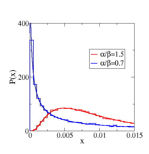
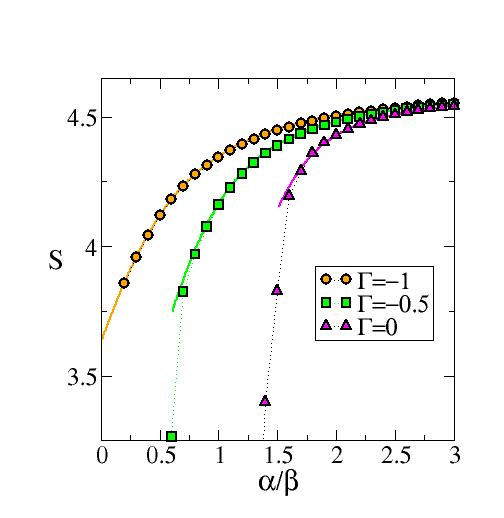
Figure 4: Test of theoretical predictions for the stable phase against simulations. The left-hand panel shows the distribution of components $x_{i}$ of mixed strategies at the fixed point ($\Gamma=-0.5$). Solid lines are theoretical predictions, noisy lines from simulations. The right-hand panel shows the entropy $S$ of the fixed point strategies of players. Symbols are from simulations (at $N=100$ strategies per player, simulations run for $7,500$ time steps, with measurements starting after $5,000$ time steps). Averages over $100$ different payoff matrices are taken. Solid lines are from the theory, hence only shown in the stable phase in the right-hand panel. Agreement with simulations is good, except for small deviations near the onset of instability. We attribute these to finite-size and equilibration effects. All data in this figure is taken at $\beta=0.01$.

D.1 Test of theoretical predictions against simulations

D.1.1 Order parameters in fixed point phase

Eqs. (62) together with Eq. (60) are the final result of our path-integral analysis in the fixed-point phase. These equations determine the relevant order parameters $\chi,q$ and $\rho$ self-consistently. We notice the high degree of nonlinearity due to the logarithmic term in (60). In absence of this term (i.e. for $r^{-1}=0$) the resulting equations are linear and the Gaussian integrals in (62) can be carried out and the resulting equations can be simplied further, see opper ; galla ; galla2 ) for details. In the presence of memory-loss ($r^{-1}>0$) this is not possible however, and we have to approach the self-consistency problem numerically. We here restrict the analysis to the case $\Gamma<0$, when a positive solution of (60) is found for all values of $z$. Numerically solving Eq. (60) gives $x(z)$ with an iterative Newton-Raphson procedure then allows us to determine the order parameters $\chi,q,\rho$ . Once these order parameters are determined the distribution of the components of the strategy vectors can be obtained from solving the above Eq. (60)

$$-r^{-1}\ln x(z)+\Gamma\chi x(z)+\sqrt{q}z-\rho=0.$$

More precisely one has

$$P(x)=\int dz\frac{e^{-z^{2}/2}}{\sqrt{2\pi}}~{}\delta(x-x(z))$$ (74)

for the distribution of fixed points of the effective process. Recalling that degrees of freedom in the path-integral analysis have been obtained from the original strategy components by a re-scaling with a factor of $N$ ($\sum_{i}x_{i}=N$ instead of $\sum_{i}x_{i}=1$), an analytical prediction for the distribution of strategy components of the original problem at a large but finite value of $N$ can be obtained using Eq. (74), and upon undoing this re-scaling. Results are shown in Fig. 4 of this Supplementary Information (left-hand panel). As seen in the figure the analytical predictions for this highly non-trivial and non-Gaussian distribution agree rather well with results from direct simulations of the original learning dynamics.

We can also determine the entropy of a typical mixed strategy of a system at finite $N$ at the fixed point as follows. Given the normalisation $\sum_{i}x_{i}=N$ we define $S$ to be the entropy of the mixed strategy vector $(x_{1}/N,\dots,x_{N}/N)$, i.e.

$$S = -\sum_{i}\frac{x_{i}}{N}\ln\frac{x_{i}}{N}$$ (75)

$$= -\frac{1}{N}\sum_{i}x_{i}\ln x_{i}+\ln(N)$$

$$= -\left\langle{x(z)\ln(x(z))}\right\rangle_{z}+\ln(N),$$

where $\left\langle{\dots}\right\rangle_{z}$ denotes an average over $z$, i.e. $\left\langle{\cdots}\right\rangle_{z}=\int dz\cdots\frac{e^{-z^{2}/2}}{\sqrt{2\pi}}$. Results are shown in Fig. 4 of this Supplementary Information (right panel), and again theoretical predictions and direct measurements from simulations agree very well. We note that mixed strategies concentrate on the centre of strategy space the for $\alpha/\beta\to\infty$, i.e. for very quick memory loss. In this case one has $x_{i}\approx 1$ for all $i$ (recall the normalisation $\sum_{i}x_{i}=N$), i.e.

$$S=-\sum_{i}\frac{x_{i}}{N}\ln\frac{x_{i}}{N}\approx-\sum_{i}\frac{1}{N}\ln\frac{1}{N}=\ln(N).$$ (76)

As a final remark we point out that Eqs. (62) and Eq. (60) are valid only in the fixed point phase, as the assumption of a fixed point was explicitly made in deriving these relations. We are therefore only able to predict the statistics of the solution in the stable fixed point phase. The solution of the effective dynamics below the transition, in the chaotic regime, is a formidable task. No promising approaches are available, similar to lack of analytical handles for example on the ‘turbulent’ so-called non-ergodic phase of the minority game coolen .

D.1.2 Onset of instability

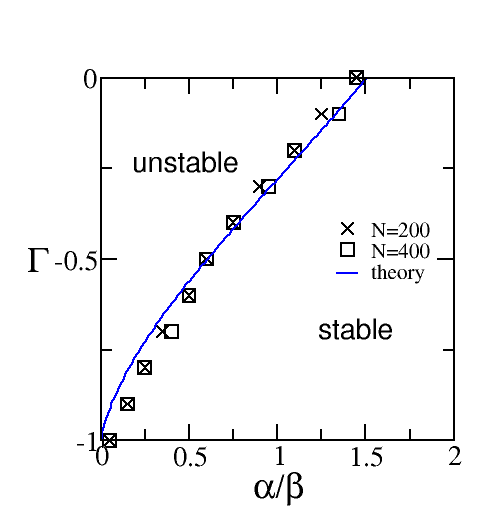
Figure 5: Test of theoretical predictions for the stability diagram. Solid line shows the onset of instability as predicted by the theory (see Eq. (73)). Markers show results from simulations (see text for details). All data in this figure is taken at $\beta=0.01$.

The validity of the analytical predictions for the onset of instability (boundary of the chaotic phase) has already been successfully confirmed in simulations in Fig. 2 of the main paper, where we have measured the expected dimension of the dynamical attractors in parameter space. These simulations are time-consuming and were therefore limited to systems of dimension $2(N-1)=98$. In order to provide a more precise verification we have determined the onset of instability in larger systems in Fig. 5 of this Supplementary Material. The numerical data is here obtained as follows:

• For a fixed value of $\Gamma$ generate $M$ samples of the payoff bi-matrix.

• For these $M$ realisations of the game, run the dynamics at large $\alpha/\beta$ and, for each sample determine whether or not it reaches a stable fixed point.

• If the majority of the $M$ samples converges to a fixed point, lower the value of $\alpha/\beta$ and repeat step 2 until more than half of the samples no longer converge.

• Record this value of $\alpha/\beta$ as the onset of instability, and proceed to a new value of $\Gamma$ in 1.

In the simulations of Fig. 5 we have used $M=10$ samples. A given run is considered to reach a fixed point if both (i) all eigenvalues of the Jacobian at a final time $T$ are within the unit circle and (ii) the total fluctuations $N^{-1}\sum_{i}\left[3/T\sum_{t=2/3T}^{T}x_{i}(t)^{2}-\left(3/T\sum_{t=2/3T}^{T}x_{i}(t)\right)^{2}\right]$ are less that a pre-defined threshold $\vartheta$. In our simulations we have used $T=15,000$ and $\vartheta=10^{-5}$. If these criteria are not fullfilled the run is considered not to converge. We cannot entirely exclude to identify runs as non-convergent, when in fact they do converge on time scales larger than $T$. In this sense we can not exclude a potential over-estimation of the value $\alpha/\beta$ at which the instability sets in in the numerical results presented in Fig. 5. The agreement with the theoretical predictions is very good however. Small deviations can be attributed to the effect just discussed, and to the fact that the theoretical prediction of the instability line is obtained for the continuous-time dynamics, whereas simulations are carried out for the discrete-time map at $\beta=0.01$. Additionally there may be potential finite size effects.

D.2 Estimation of the attractor dimension

The Liapunov spectrum of the attractors are determined using a procedure similar to that described in sandri . Measurements are started after some equilibration time ($t_{\mbox{eq}}=150,000$ iterations), after which we run a linearised map

$$\mathbf{z}(t+1)=J_{\mathbf{x}(t),\mathbf{y}(t)}\mathbf{z}(t),$$ (77)

parallel to the simulation of the original system, with $L=2(N-1)$ degrees of freedom. The $L\times L$ matrix $J_{\mathbf{x}(t),\mathbf{y}(t)}$ is the Jacobian of the full non-linear system. We run $L$ copies of the linearized dynamics, $z^{(1)},\dots,z^{(L)}$ started from the $L$ unit vectors. We then regularly perform a stabilized Gram-Schmidt procedure, and obtain estimates of the Liapunov exponents sandri . From these estimates one then calculates the Kaplan-Yorke dimension as

$$D=j-\frac{\sum_{i=1}^{j}\lambda_{i}}{\lambda_{j+1}},$$ (78)

where the Liapunov exponents are ordered as $\lambda_{1}\geq\lambda_{2}\geq\dots\geq\lambda_{L}$, and where $j$ is the largest integer such that $\lambda_{1}+\dots+\lambda_{j}\geq 0$ kaplan ; sandri . The estimates of the attractor dimension may fluctuate as the simulation run continues after equilibration, and as the attractor is sampled. In practice we find that the measured dimension tends to converge in most runs as the duration of the simulation increases. In our simulations we consider the attractor dimension in a given run as converged when the difference between the maximum and minimum estimate of the dimension in a time window of $20,000$ iteration steps deviate by less than $5\%$ from each other. The dimension reported is then the average over that time window. In other words, simulations are first run for $150,000$ steps to equilibrate, then at least $20,000$ iterations additional are performed during which measurements are taken. Subsequently the simulation is extended (up to at most $10^{6}$ iterations) until the convergence criterion is met. In practice we find that most samples have converged at $10^{6}$ iterations or earlier, when we terminate our simulation. Examples of such measurements are shown in Fig. 6 of this Supplementary Information, the data shown corresponds to the attractors shown in Fig. 1 of the main paper. Samples that have not converged on this time scale are ignored in our analysis, and have been disregarded when compiling the data for Fig. 2 of the main paper. We here find that only a small fraction of samples converges when the attractor dimension is very high.

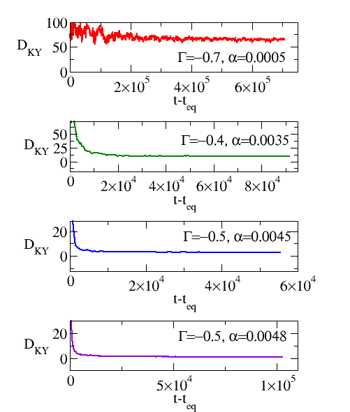
Figure 6: Convergence of measurements of attractor dimensions. Data is from simulations of games with $N=50$ strategies per player, and corresponds to the four attractors shown in Fig.1 of the main manuscript.

D.3 Return distribution

The time series of ‘returns’ in Fig. 3 of the main manuscript shows the changes of total payoff to the two players. Specifically, we measure

$$\Pi_{\mbox{{\small tot}}}(t)=\sum_{i}\sum_{j}\left\{x_{i}(t)a_{ij}y_{j}(t)+y_{i}(t)b_{ij}x_{j}(t)\right\}$$ (79)

at each time step $t$ in the equilibrated regime, and then plot $\Pi_{\mbox{{\small tot}}}(t)-\Pi_{\mbox{{\small tot}}}(t-1)$ in Fig. 3 of the main paper. The corresponding distribution of returns is shown in Fig. 7 of this SI, and shows exponential tails.

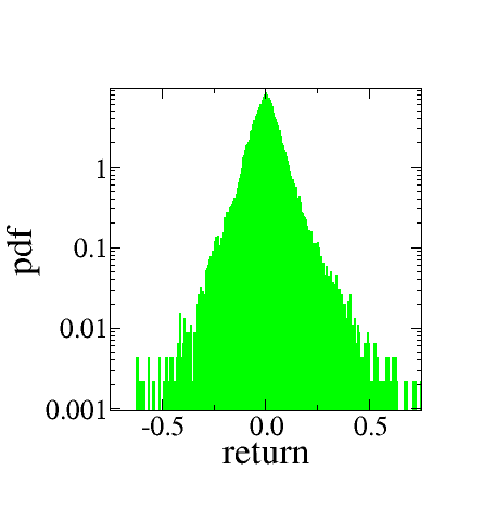
Figure 7: Distribution of returns for the run shown in Fig. 3 of the main manuscript.

References

• (1) J. Nash, Equilibrium points in n-person games, Proceedings of the National Academy of Sciences 36 (1) 48-49 (1950)
• (2) J. von Neumann, O. Morgenstern, Theory of Games and Economic Behaviour, Princeton University Press, Princeton NJ (2007)
• (3) A. McLennan, J. Berg, The asymptotic expected number of Nash equilibria of two player normal form games, Games and Economic Behavior 51(2), 264-295 (2005)
• (4) J. Berg, M. Weigt, Entropy and typical properties of Nash equilibria in two-player Games, Europhys. Lett. 48(2), 129-135 (1999).
• (5) M. Opper, S. Diederich, Phase transition and $1/f$ noise in a game dynamical model, Phys. Rev. Lett. 69 1616-1619 (1992)
• (6) S. Diederich, M. Opper, Replicators with random interactions: A solvable model, Phys. Rev. A 39 4333-4336 (1989).
• (7) T. H. Ho, C. F. Camerer, J.-K. Chong, Self-tuning experience weighed attraction learning in games, J. Econ. Theor. 133 177-198 (2007)
• (8) C. Camerer, T.H. Ho, Experience-weighted attraction learning in normal form games, Econometrica 67 (1999) 827
• (9) C. Camerer, Behavioral Game Theory: Experiments in Strategic Interaction (The Roundtable Series in Behavioral Economics), Princeton University Press, Princeton NJ, 2003
• (10) D. Fudenberg, D.K. Levine, Theory of Learning in Games, MIT Press, Cambridge MA (1998)
• (11) H. P. Young, Individual Strategy and Social Structure: An Evolutionary Theory of Institutions, Princeton University Press, Princeton NJ (1998)
• (12) W. A. Brock, C. H. Hommes, Heterogeneous beliefs and routes to chaos in a simple asset pricing model, J. Econ. Dyn. and Contr. 22 1235-1274 (1998)
• (13) B. Skyrms, Chaos in game dynamics, J. of Logic, Language and Information 1 111-130 (1992)
• (14) Y. Sato, E. Akiyama, J. D. Farmer, Chaos in learning a simple two-player game, Proc. Nat. Acad. Sci. USA 99 4748-4751 (2002)
• (15) Y. Sato, J.-P. Crutchfield, Coupled replicator equations for the dynamics of learning in multiagent systems, Phys. Rev. E 67 015206(R) (2003)
• (16) M. A. Nowak, Evolutionary dynamics, Harvard University Press, Cambridge MA (2006)
• (17) J. Hofbauer, K. Sigmund, Evolutionary games and population dynamics, Cambridge University Press, Cambridge, 1998
• (18) R. M. May, Will a Large Complex System be Stable? Nature 238, 413 - 414 (1972);
• (19) Note that the fixed point reached in the stable regime is only a Nash equilibrium at $\Gamma=0$ and in the limit $\alpha\to 0$. When $\alpha>0$ the players are effectively assuming their opponent’s behavior is non-stationary, and that more recent moves are more useful than moves in the distant past.
• (20) DeΒ Dominicis, C., Phys. Rev. B 18 4913-4919 (1978)
• (21) Ghashghaie, S., Breymann, W., Peinke, J., Talkner, P., Dodge, Y., Turbulent cascades in foreign exchange markets, Nature 381 767-770 (1996)
• (22) In contrast to financial markets, for the behavior we observe here the distribution of heavy tails decay exponentially (as opposed to following a power law). We hypothesize that this is because the players in financial markets use a variety of different timescales $\alpha$.
• (23) Lorenz, E. N., Atmospheric predictability revealed by naturally occurring analogues, J. Atmos. Sci. 26, 636-646 (1969)
• (24) J. D. Farmer, J. J. Sidorowich, Predicting chaotic time series, Phys. Rev. Lett. 59 845-848 (1987)
• (25) T . H. Ho, C. F. Camerer, J.-K. Chong, Self-tuning experience weighted attraction learning in games, J. Econ. Theory 133 (2007) 177
• (26) Y. Sato. D. Farmer, in preparation
• (27) T. Galla, Intrinsic noise in game dynamical learning, Phys. Rev. Lett. 103 (2009) 198702
• (28) J. Realpe-Gomez J. et al., Fixation and escape times in stochastic game learning, submitted (2011), preprint available at http://arxiv.org/abs/1102.0876
• (29) T. Galla, Cycles between cooperation and defection in imperfect learning, submitted 2011, preprint available at http://arxiv.org/abs/1101.4378
• (30) D. Vilone, A. Robledo, A. Sanchez, Chaos and unpredictability in evolutionary games in discrete time, preprint http://arxiv.org/abs/1103.1484
• (31) G. Parisi, M. Mezard, M. A. Virasoro, Spin glass theory and beyond, World Scientific Publishing, Singapore (1987)
• (32) A. C. C. Coolen, in Handbook of Biological Physics Vol 4 (Elsevier Science 2001; eds. F. Moss and S. Gielen), 597-662 Statistical mechanics of Recurrent Neural networks II: Dynamics
• (33) A. C. C. Coolen, The mathematical theory of minority games, Oxford University Press, Oxford UK (2005)
• (34) M. Opper, S. Diederich, Replicator Dynamics, Computer Physics Communications Volumes 121-122, September-October 1999, Pages 141-144 Proceedings of the Europhysics Conference on Computational Physics CCP 1998
• (35) T. Galla, Random replicators with asymmetric couplings, J. Phys. A: Math. and Gen. 39 3853 (2006)
• (36) T. Galla, Two-population replicator dynamics and number of Nash equilibria in matrix games, EPL (Europhysics Letters) 78 20005 ( 2007)
• (37) T. Galla, A. C. C. Coolen, D. Sherrington, Dynamics of a spherical minority game, J . Phys. A: Math. Gen. 36 (2003) 11159-11172
• (38) M. Sandri, Numerical calculation of Lyapunov exponents, The Mathematica Journal 6, 78-84 (1996)
• (39) J. Kaplan, J. A. Yorke, In Functional Differential Equations and Approximations of Fixed Points: Proceedings, Bonn, July 1978 (Ed. H.-O. Peitgen and H.-O. Walther). Berlin: Springer-Verlag, p. 204, 1979.