Metastates in mean-field models with random
external fields generated by Markov chains

Abstract

We extend the construction by Külske and Iacobelli of metastates in finite-state mean-field models in independent disorder to situations where the local disorder terms are a sample of an external ergodic Markov chain in equilibrium. We show that for non-degenerate Markov chains, the structure of the theorems is analogous to the case of i.i.d. variables when the limiting weights in the metastate are expressed with the aid of a CLT for the occupation time measure of the chain.
As a new phenomenon we also show in a Potts example that for a degenerate non-reversible chain this CLT approximation is not enough, and that the metastate can have less symmetry than the symmetry of the interaction and a Gaussian approximation of disorder fluctuations would suggest.

AMS 2000 subject classification: 82B44, 82B26, 60K35.

Keywords: Gibbs measures, mean-field systems, disordered systems, metastates, Markov chains, Ising model, Potts model.

1 Introduction

Metastates are useful concepts in analyzing the large-volume dependence of disordered systems, both of lattice and mean-field systems. They go back to the constructions of Aizenman and Wehr [1], and Newman and Stein [18].

In the present paper we continue to analyze a class of mean-field systems, moving from a situation where the quenched disorder was assumed to be i.i.d. [11] to a situation where the disorder is generated by a Markov chain. Our models have a finite local state space $E$, and a finite space $E^{\prime}$ of possible values of the local disorder variables. While in the previous analysis the disorder variables were assumed to be i.i.d. over the sites, we now treat a quenched disorder which is correlated and generated by a Markov chain with transition matrix $M$. For a study of the Curie-Weiss model in a dynamical external field see [8, 20].

A metastate is a probability measure on the infinite-volume Gibbs measures of a disordered system which intuitively gives the likehood to pick a Gibbs state in a large but finite volume. For precise definitions see below and refer to the books [4, 17]. Non-trivial metastates can occur when the phenomenon of random symmetry breaking appears, meaning that two or more states are equivalent on the average, but their symmetry is broken by disorder fluctuations in finite volume. For examples of disordered models with such random symmetry breaking see [5, 6, 10, 13, 14, 15], for genuine applications of metastate idea to spin-glasses see [16, 19] and in particular the groundstate uniqueness result in 2D proved in [3].

Now, in the finite-type mean-field models of [11] precise limit theorems for the weights in the metastates were derived, combining a multivariate CLT for disorder fluctuations and a large-deviation analysis of the spin-part of the model. Further a geometric picture was given to identify the invisible states, namely those Gibbs states which are always overshadowed by disorder fluctuations favoring other competing states.

In the present paper we ask: What changes if the external randomness comes from a Markov Chain?

Suppose we are dealing with a non-degenerate Markov chain on a finite state-space at first, meaning that the covariance matrix $\Sigma_{M}$ of the limiting Gaussian distribution of the occupation time-vector of the Markov chain $M$ has the full possible rank. Then the basic structure of the theorems stays the same, using the same geometric construction to identify visible Gibbs states $j$ and their weights $w_{j}$. However, let us stress the main difference to the independent case, which is that the $w_{j}$’s are given in terms of $\Sigma_{M}$ and this object carries more information about the Markov chain then just its invariant distribution $\pi$. Which states are Gibbs states depends on $\pi$, but the precise form of the weights and whether a given state is visible or not can vary over Markov chains having the same $\pi$ but different transition matrix $M$. This is different from the i.i.d. case where the single-site distribution $\pi$ completely specifies the disorder distribution.

New phenomena on an even more fundamental level appear when we allow for Markov chains which are degenerate, i.e., whose $\Sigma_{M}$ does not have full rank. We specify to a concrete example and look at the 3-state random field Potts model, with $3$-state local random fields coupling by delta-interaction in the Hamiltonian to the spins. We take $M$ on $E^{\prime}=\{1,2,3\}$ to be doubly stochastic ergodic matrix which can be seen as a softened version of a permutation matrix, where one keeps however one (and only one) transition between an ordered pair of states to be deterministic, say from state $1$ to $2$. Although the equidistribution on the states is invariant and the covariance matrix $\Sigma_{M}$ becomes degenerate but is symmetric under exchange of states $1$, and $2$, the metastate for the random model with disorder generated by the Markov chain in equilibrium is not symmetric under an exchange of the spin labels $1$ and $2$. Such a phenomenon is only possible because of two features: The almost degeneracy between two Gibbs-states up to finite but non-zero free energy differences in arbitrary large volumes in the possible realizations of the chain, and the lack of time-reversal symmetry of the Markov chain.

The remainder of the paper is organized as follows. In Section 2 we review definitions about metastates and the constructions from [11] needed for mean-field models, including the geometry of free energy fluctuations and derivation of weights for pure states. Then we are ready to give the result of the present paper about metastates for non-degenerate Markov chains. Next we present the results for the $3$-state Potts model with quenched disorder generated by a degenerate chain. In Section 3 the proofs for non-degenerate Markov chains are given, building on results of the previous paper [11]. In Section 4 the proof for the $3$-state Potts model in the degenerate case is given.

2 Main Results

2.1 Mean-field Spin Models in a random field generated by a Markov chain

2.1.1 The Boltzmann distribution of the spins

For spin variables $\sigma(i)$, at each site $i\in\{1,\dots,n\}$ taking values in a finite set $E$, we consider a mean-field model with Hamiltonian $nF(\nu)$, and Boltzmann distribution given by:

$$\begin{split}&\mu_{F,n}[\eta(1),\ldots,\eta(n)](\sigma(1)=\omega(1),\dots,\sigma(n)=\omega(n))\cr&=\frac{1}{Z_{n}[\eta(1),\ldots,\eta(n)]}\exp\left(-nF(L_{n}^{\omega})\right)\prod_{i=1}^{n}\alpha[\eta(i)](\omega_{i})\cr\end{split}$$ (2.1)

where $L_{n}^{\omega}=\frac{1}{n}\sum_{i=1}^{n}\delta_{\omega(i)}$ is the empirical spin distribution. The Boltzmann distribution depends on the quenched disorder $\eta(1),\ldots,\eta(n)$ via the a-priori distribution $\alpha[b]\in\mathcal{P}(E)$, $b\in E^{\prime}$, where the type-space $E^{\prime}$ of the local disorder variables is taken to be finite. Throughout the paper we use the notation ${\cal P}(\hat{E})$ for the probability measures on a space $\hat{E}$, not mentioning the sigma-algebra explicitly unless necessary.

2.1.2 The Markov chain of the disorder variables

Let the probability distribution of the disorder be given by a Markov chain on the finite space $E^{\prime}$ with transition matrix $M$ and invariant measure $\pi$, written in vector notation as $\pi^{t}M=\pi^{t}$ where $t$ denotes transposition of the column vector $\pi$. The chain is supposed to be in equilibrium, i.e. the initial state $\eta(0)$ is chosen according to the invariant distribution of the chain $\pi\in\mathcal{P}(E^{\prime})$, and ${\mathbb{P}}_{\pi}$ is the corresponding measure on $(E^{\prime})^{{\mathbb{N}}}$, that is the one with ${\mathbb{P}}_{\pi}(\eta(i+1)=b^{\prime}|\eta(i)=b)=M(b,b^{\prime})$ and ${\mathbb{P}}_{\pi}(\eta(i)=b)=\pi(b)$ for all $i\in{\mathbb{N}}$ and $b\in E^{\prime}$. We will assume that the transition matrix $M$ is ergodic, meaning that there exists a power $M^{r}$ for which all matrix elements are strictly bigger than zero.

Given the first $n$ realizations of the Markov chain $\eta$ we denote by

$$\Lambda_{n}(b)=\{i\in\{1,\dots,n\}:\eta(i)=b\}$$

the set of $b$-like sites, $b\in E^{\prime}$. Then the number $|\Lambda_{n}(b)|$ is the occupation-time of the chain at state $b$ up to “time” $n$, and the normalized expression

$$\hat{\pi}_{n}(b)=\frac{|\Lambda_{n}(b)|}{n}$$

is the relative frequency of $b$-like sites in the sample. The empirical spin distribution on the $b$-like sites is given by

$$\hat{L}_{n}(b)=\frac{1}{|\Lambda_{n}(b)|}\sum_{i\in\Lambda_{n}(b)}\delta_{\omega(i)}$$

and moreover the total empirical spin distribution can be written as the scalar product of $\hat{\pi}_{n}$ and $\hat{L}_{n}$, i.e.

$$L_{n}=\sum_{b\in E^{\prime}}\hat{\pi}_{n}(b)\hat{L}_{n}(b).$$

The equilibrium states of the system are given by the minimizers of the free energy functional [11]

$$\hat{\nu}\mapsto\varphi[\pi](\hat{\nu})$$ (2.2)

where

$$\begin{split}&\varphi:\mathcal{P}(E^{\prime})\times\mathcal{P}(E)^{E^{\prime}}\rightarrow{\mathbb{R}},\cr&\varphi[\pi](\hat{\nu})=F\left(\sum_{b\in E^{\prime}}\hat{\pi}(b)\hat{\nu}(b)\right)+\sum_{b\in E^{\prime}}\hat{\pi}(b)S\left(\hat{\nu}(b)|\alpha[b]\right).\cr\end{split}$$ (2.3)

Here, $S(p_{1}|p_{2})=\sum_{a\in E}p_{1}(a)\log\frac{p_{1}(a)}{p_{2}(a)}$ is the relative entropy.

Together with the free energy we consider its linearization at some fixed minimizer $\hat{\nu}_{j}$ as a function of $\pi$, which reads as follows

$$\varphi[\tilde{\pi}](\hat{\nu}_{j})-\varphi[\pi](\hat{\nu}_{j})=-B_{j}[\tilde{\pi}-\pi]+o(||\tilde{\pi}-\pi||)$$ (2.4)

As in [11], throughout the present paper we restrict ourselves to the following non-degeneracy conditions:

1. the set $M^{*}$ of minimizers of the free energy is finite and the Hessian is positive at each minimizer.

2. No different minimizers $\hat{\nu}_{i}$ and $\hat{\nu}_{j}$ have the same $B_{i}=B_{j}$.

Our first results concern the metastate on the level of the empirical spin-distribution. Denote by $\rho[\eta](n):=\mu_{F,n}[\eta](L_{n})\in{\cal P}({\cal P}(E))$ the distribution of $L_{n}$ under the finite-volume Gibbs-measure. The concentration of these measures around the finitely many minimizers of the free energy function $\pi M^{*}=\{\pi\hat{\nu}_{j},j=1,\dots,k\}$ holds by assumption. How this concentration takes place in asymptotically large volumes is made precise by the following definition of a metastate.

Definition 2.1

Assume that for every bounded continuous $\psi:\mathcal{P}\left({\mathcal{P}}(E)\right)\times(E^{\prime})^{\infty}\rightarrow{\mathbb{R}}$ the limit

$$\lim_{n\rightarrow\infty}\int{\mathbb{P}}(d\eta)\psi(\rho[\eta](n),\eta)=\int K\left(d\rho,d\eta\right)\psi(\rho,\eta)$$ (2.5)

exists. Then the conditional distribution $\kappa[\eta](d\rho)=K(d\rho|\eta)$ is called the metastate on the level of the empirical distribution.

Before stating the theorem we must introduce the definition of the region of stability for the minimizers:

Definition 2.2

Let us define the set

$$R_{j}:=\{x\in T\mathcal{P}(E^{\prime}),\langle x,B_{j}\rangle>\max_{k\neq j}\langle x,B_{k}\rangle\}$$ (2.6)

where $T\mathcal{P}(E^{\prime})=\{x=(x(1),\ldots,x(|E^{\prime}|)):\sum_{i=1}^{|E^{\prime}|}x(i)=0\}$ is the tangent space of field type measures. We say that $R_{j}$ is the stability region of $\hat{\nu}_{j}$.

We will use the following CLT for the occupation time measure (see Appendix).

Fact: For an ergodic finite-state Markov chain, the standardized occupation-time fluctuation measure $\sqrt{n}(\hat{\pi}_{n}-\pi)$ converges in distribution, as $n$ tends to infinity, to a centered Gaussian distribution $G$ with a covariance matrix $\Sigma_{M}$ on the $|E^{\prime}|-1$ dimensional vector space $T\mathcal{P}(E^{\prime})$.

Warning: Ergodicity of the Markov chain does not imply that $\Sigma_{M}$ has the full rank $|E^{\prime}|-1$, we will discuss in detail an example where this is not the case. In generalization of the case of i.i.d. $\eta(i)$’s we have the following result.

Theorem 1

Consider a mean-field model with quenched disorder generated by an ergodic finite state Markov chain $M$ in equilibrium $\pi$, with full rank occupation-time covariance $\Sigma_{M}$. Suppose the non-degeneracy conditions 1. and 2. on the spin model (see pag.2.4). Then the metastate on the empirical spin-measure exists and takes the form

$$\kappa[\eta](d\rho)=\sum_{j=1}^{k}w_{j}\delta_{\delta_{\pi\hat{\nu}_{j}}}(d\rho)\mbox{ for ${\mathbb{P}}_{\pi}$-a.e. $\eta$.}$$ (2.7)

The weights are $w_{j}={\mathbb{P}}_{\Sigma_{M}}(G\in R_{j})$ where $G$ is a centered Gaussian on $T\mathcal{P}(E^{\prime})$ with covariance $\Sigma_{M}$.

As in the case for i.i.d. $\eta(i)$’s we also have the analogous version for the metastate on the level of spin distributions. We call a function on an infinite product of a finite space continuous (w.r.t. local topology) if it is a uniform limit of local functions. For probability measures on ${\cal P}(E^{\infty})$ we use the weak topology (according to which a sequence of measures converges iff it converges on continuous test-functions), and for ${\cal P}(E^{\infty})\times(E^{\prime})^{\infty}$, we use the product topology.

Definition 2.3

Assume that, for every bounded continuous $\Xi:{\cal P}(E^{\infty})\times(E^{\prime})^{\infty}\rightarrow{\mathbb{R}}$ the limit

$$\begin{split}&\lim_{n\uparrow\infty}\int{\mathbb{P}}(d\eta)\Xi(\mu_{n}[\eta],\eta)=\int J(d\mu,d\eta)\Xi(\mu,\eta)\cr\end{split}$$ (2.8)

exists. Then the conditional distribution $\kappa[\eta](d\mu):=J(d\mu|\eta)$ is called the AW-metastate on the level of the states.

Theorem 2

In the situation of Theorem 1, the metastate on the level of the states equals

$$\begin{split}&\kappa[\eta](d\mu)=\sum_{j=1}^{k}w_{j}\delta_{\mu_{j}[\eta]}(d\mu)\end{split}$$ (2.9)

with the product measures $\mu_{j}[\eta]:=\prod_{i=1}^{\infty}\gamma[\eta(i)](\,\cdot\,|\pi\hat{\nu}_{j})$ given by the kernels

$$\begin{split}\gamma[b](a|\nu)=\frac{e^{-dF_{\nu}(a)}\alpha[b](a)}{\sum_{\bar{a}\in E}e^{-dF_{\nu}(\bar{a})}\alpha[b](\bar{a})}\end{split}$$ (2.10)

where $dF_{\nu}(a)$ is the $a$-th coordinate of the differential of the function $F$ on ${\cal P}(E)$ taken at the point $\nu\in{\cal P}(E)$.

The proofs of these theorems are analogous to the i.i.d. case, however with some additional features when decoupling properties of random field realizations in separate finite volumes need to be treated.

2.2 Potts model in a random-field generated by a degenerate Markov chain

The random-field Potts model of the form we consider is given by the energy

$$F(\nu)=-\frac{\beta}{2}(\nu(1)^{2}+\dots+\nu(q)^{2})$$

where $E\equiv E^{\prime}=\{1,\dots,q\}$ and the random fields couple locally to the spins via the local measures $\alpha[b](a)=\frac{e^{B1_{b=a}}}{e^{B}+q-1}$. We will consider a Markov chain $M$ with invariant measure $\pi$ given by the equidistribution.

The structure of the phases depends on $M$ only through $\pi$ and the case of i.i.d. equidistributed variables has already been treated in [11], so let us recall the relevant information from there: The total empirical distribution of the minimizers of the free energy functional has the form $\nu_{j,u}\in{\cal P}(E)$, with possible order in direction $j$, such that $\nu_{j,u}(j)=\frac{1+u(q-1)}{q}$, $\nu_{j,u}(i)=\frac{1-u}{q}$ for $i\neq j$, where the symmetry-breaking parameter $u$ obeys the mean-field equation

$$\begin{split}u&=\frac{e^{\beta u}}{e^{\beta u}+e^{B}+(q-2)}-\frac{1}{e^{\beta u+B}+(q-1)}\end{split}$$ (2.11)

In a region of small $B$ and large $\beta$ there is a non-zero solution of this mean-field equation; to decide whether this or the zero solution corresponds to the global minimizer one looks at the corresponding free energy which reads

$$\begin{split}&\log\frac{e^{B}+q-1}{e^{\beta u}+e^{B}+q-2}+\frac{\beta(q-1)}{2q}u^{2}+\frac{\beta}{q}u-\frac{1}{q}\log\frac{e^{\beta u+B}+q-1}{e^{\beta u}+e^{B}+q-2}\end{split}$$ (2.12)

There is a curve in the $(\beta,B)-$plane when there is an equal-depth minimum at $u=0$ and a positive value of $u=u^{*}(\beta,q)$. This means that on this curve there is a coexistence of $q$ ordered states and one disordered state where $u=0$ in the random model in the very same way as it is happening for the nonrandom model where $B=0$.

The stability vector for the state $\nu_{1,u}$ is

$$\begin{split}\hat{B}_{\nu_{1,u}}=\begin{pmatrix}\frac{q-1}{q}\log\frac{e^{\beta u+B}+q-1}{e^{\beta u}+e^{B}+q-2}\\ -\frac{1}{q}\log\frac{e^{\beta u+B}+q-1}{e^{\beta u}+e^{B}+q-2}\\ \dots\\ -\frac{1}{q}\log\frac{e^{\beta u+B}+q-1}{e^{\beta u}+e^{B}+q-2}\end{pmatrix}\cr\end{split}$$

pointing into the direction $1$ in $T{\cal P}(E^{\prime})$ which is intuitively clear since a majority of $1$-type random fields favor the state having a majority of $1$-type spins. The other stability vectors are given by permutation.

Let us specialize to $q=3$. In the case of i.i.d. random fields the metastate on the spin-distributions becomes

$$\kappa[\eta](d\mu)=\frac{1}{3}\sum_{j=1}^{3}\delta_{\mu_{j}[\eta]}$$

with $\mu_{j}[\eta]=\prod_{i=1}^{\infty}\gamma[\eta(i)](\,\cdot\,|\nu_{j,u=u^{*}(\beta,q)})$. In particular the state for $u=0$ is invisible. This follows since the stability vector for this state must vanish, by symmetry, as was explained in the previous paper.

We note that the form of the minimizers and the stability vectors depend only on $\pi$. So, equally for a Markov chain $M$ which has the equidistribution as its invariant measure, and has a non-degenerate covariance matrix $\Sigma_{M}$ the state for $u=0$ will stay invisible, and the metastate will become

$$\kappa[\eta](d\mu)=\sum_{j=1}^{3}w_{j}\delta_{\mu_{j}[\eta]}$$ (2.13)

with weights $w_{1},w_{2},w_{3}$ which are given by the probabilities of finding a (in general non-isotropic) Gaussian in the corresponding equal-sized stability regions, see (4.2). Hence in general the $w_{1},w_{2},w_{3}$ will be different.

The form (2.13) changes completely, in that the metastate is now supported on mixed states, when we consider, for $p\in(0,1)$ the following degenerate (but ergodic) Markov chain which also has the equidistribution as its invariant measure.

$$M=\left(\begin{matrix}0&1&0\\ p&0&1-p\\ 1-p&0&p\\ \end{matrix}\right)$$ (2.14)

Figure 1: The transition graph for matrix (2.14) with a deterministic transition from state 1 to state 2.

The result for the metastate takes the following surprising form.

Theorem 3

The metastate in the $3$-state random-field Potts model defined above, with a random-field generated by the Markov chain $M$ of eq. (2.14), has the form

$$\kappa[\eta]=\frac{1}{2}\delta_{\mu^{3}[\eta]}+\frac{1}{3}\delta_{\frac{1}{2}\mu^{1}[\eta]+\frac{1}{2}\mu^{2}[\eta]}+\frac{1}{9}\delta_{p(\beta,B)\mu^{1}[\eta]+(1-p(\beta,B))\mu^{2}[\eta]}+\frac{1}{18}\delta_{(1-p(\beta,B))\mu^{1}[\eta]+p(\beta,B)\mu^{2}[\eta]}$$ (2.15)

Here the function $p(\beta,B)$ is computable in terms of the mean-field parameter $u$ and is strictly bigger than $1/2$ in the phase transition regime.

Note that the metastate is supported not only on pure states but also on mixtures, and moreover the weights are non-symmetric under exchange of the state $1$ and $2$.

Note that if we tried to apply Theorem 2 to the case of the degenerate chain we would find a Gaussian for the disorder fluctuations in the two-dimensional space $T{\cal P}(E^{\prime})$ which is supported by the one-dimensional sub-space which contains the boundary between the stability regions for the states $\mu^{1}[\eta]$ and $\mu^{2}[\eta]$, see Figure 2. Hence the pure state $\mu^{3}[\eta]$ should occur with a weight of $1/2$ in the metastate. In order to make statements about the occurrence of mixtures of $\mu^{1}[\eta]$ and $\mu^{2}[\eta]$ and their weights the refined analysis of Section 4 is needed.

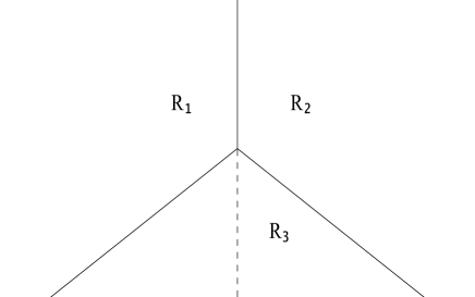
Figure 2: The Gaussian limiting distribution of $\sqrt{n}(\hat{\pi}_{n}-\pi)$ concentrates on the dashed line that for upper half coincides with the boundary between the stability regions $R_{1}$ and $R_{2}$.

3 Metastates for non-degenerate Markov Chains: Proof

The proof of Theorem 1 in the case of i.i.d. distributed disorder variables relies in an essential way on the product nature of the disorder measure. The main step in the present case is a modification of Lemma 2.10 in [11] to the dependent case. For the rest, our argument follows closely the proof of Külske and Iacobelli, and we give details only where the dependence of the disorder variables come into play. Nevertheless, for the sake of completeness we recall some notation and results from [11].

Once we have the CLT for the empirical measure, the weights $w_{j}$ come from the study of the limiting probability of the $n,l$-dependent good sets ${\cal H}_{i,n,l}^{\tau}$ of the realization of the randomness. For $n_{1}<n_{2}$, let us put

$$X_{[n_{1},n_{2}]}[\eta]=\frac{1}{\sqrt{n_{2}-n_{1}+1}}\sum_{i=n_{1}}^{n_{2}}\delta_{\eta_{i}}-\sqrt{n_{2}-n_{1}+1}\pi$$ (3.1)

and define $n,l$-dependent good-sets ${\cal H}_{i,n,l}^{\tau}$ of the realization of the randomness as follows

$$\begin{split}&{\cal H}_{i,n,l}^{\tau}:=\left\{\eta\in(E^{\prime})^{n-l}:X_{[l+1,n]}[\eta]\in R_{i,n}^{\tau}\right\}\cr&{\cal H}_{n,l}^{\tau}:=\bigcup_{i=1}^{k}{\cal H}_{i,n,l}^{\tau}\end{split}$$ (3.2)

where $R_{i,n}^{\tau}:=\{x\in T{\cal P}(E^{\prime}):\langle x,B_{i}\rangle-\max_{k\neq i}\langle x,B_{k}\rangle>n^{-\frac{1}{2}+\tau},\|x\|\leq n^{\frac{\tau}{4}}\}$, where $0<\tau<\frac{1}{2}$. The set ${\cal H}_{i,n,l}^{\tau}$ of the disorder random variables allows to deduce that the measure on the empirical distribution will be concentrated inside a ball around the minimizer $\pi\hat{\nu}^{*}_{i}$. A similar concentration takes place for averages of continuous test-functions with respect to the empirical spin-distribution (see [11] for a proof).

Lemma 3.1

For any real-valued continuous function $g$ on ${\cal P}(E)$ the following concentration property holds:

$$|\rho[\eta](n)(g)-g(\pi\hat{\nu}_{j}^{*})|\leq\tilde{r}(n),\quad\forall\,\eta\in{\cal H}_{j,n,0}^{\tau},$$ (3.3)

where $\lim_{n\rightarrow\infty}\tilde{r}(n)=0$.

The fundamental property of the good sets is that their probability does not depend on any finite number $l$ of sites in the limit $n\rightarrow\infty$. In order to make this precise, the authors in [11] considered sligthly different sets. For any $l<n$, we define a subregion ${\cal H}_{i,n,0}^{\tau}(l)$ of ${\cal H}_{i,n,0}^{\tau}$, as follows

$$\begin{split}&{\cal H}_{i,n,0}^{\tau}(l):=\biggl{\{}\eta\in(E^{\prime})^{n}:\cr&a_{n}\langle X_{[1,l]}[\eta],B_{i}\rangle+b_{n}\langle X_{[l+1,n]}[\eta],B_{i}\rangle-\max_{k\neq i}\left(a_{n}\langle X_{[1,l]}[\eta],B_{k}\rangle\right)-\max_{k\neq i}\left(b_{n}\langle X_{[l+1,n]}[\eta],B_{k}\rangle\right)>{\delta_{n}},\cr&\text{ and }\|X_{[1,n]}[\eta]\|\leq n^{\frac{\tau}{4}}\biggr{\}}\cr\end{split}$$ (3.4)

where $a_{n}=\frac{\sqrt{nl}}{n}$ and $b_{n}=\frac{\sqrt{n(n-l)}}{n}$.

The properties and the relations between ${\cal H}_{i,n,0}^{\tau}$ and ${\cal H}_{i,n,0}^{i}(l)$ are summarized in the following lemmas. We refer to [11] for the details.
Our first lemma states that for any fixed integer $l$, there is a subregion of the good-set which will not play any role in the limit $n\uparrow\infty$.

Lemma 3.2

For any integer $l$, ${\mathbb{P}}({\cal H}_{i,n,0}^{\tau}\setminus{\cal H}_{i,n,0}^{\tau}(l))$ goes to zero in the limit $n\uparrow\infty$.

We also need the sets

$$\begin{split}&B_{i,n}^{{\tau}}(l)=(E^{\prime})^{l}\times{\cal H}_{i,n,l}^{1,\tau}\cr&A_{i,n}^{{\tau}}(l)=(E^{\prime})^{l}\times{\cal H}_{i,n,l}^{2,\tau}\cr\end{split}$$ (3.5)

where

$$\begin{split}&{\cal H}_{i,n,l}^{1,\tau}=\biggl{\{}\eta\in(E^{\prime})^{n-l}:\varphi^{i}(X_{[l+1,n]}[\eta])>b_{n}^{-1}\left({\delta_{n}}+a_{n}C_{2}(l)\right),\text{ and }\|X_{[l+1,n]}[\eta]\|\leq b_{n}^{-1}(n^{\frac{\tau}{4}}-\tilde{C}_{2}(l))\bigg{\}}\cr&{\cal H}_{i,n,l}^{2,\tau}=\biggl{\{}\eta\in(E^{\prime})^{n-l}:\varphi^{i}(X_{[l+1,n]}[\eta])>b_{n}^{-1}\left({\delta_{n}}-a_{n}C_{2}(l)\right),\text{ and }\|X_{[l+1,n]}[\eta]\|\leq b_{n}^{-1}n^{\frac{\tau}{4}}\bigg{\}}\cr\end{split}$$ (3.6)

with the definitions

$$\varphi^{i}(X_{[l+1,n]}[\eta]):=\langle X_{[l+1,n]}[\eta],B_{i}\rangle-\max_{k\neq i}\langle X_{[l+1,n]}[\eta],B_{k}\rangle$$ (3.7)

and

$$\begin{split}&C_{2}(l)=\sqrt{l}\max_{\eta}\left|\max_{k\neq i}\langle X_{[1,l]}[\eta],B_{k}\rangle-\langle X_{[1,l]}[\eta],B_{i}\rangle\right|\cr&\tilde{C}_{2}(l)=\max_{\eta}||X_{[1,l]}[\eta]||.\cr\end{split}$$ (3.8)

The following holds:

1. From the definitions follow

   $$\begin{split}&A_{i,n}^{{\tau}}(l)\supseteq{\cal H}_{i,n,0}^{\tau}(l)\supseteq B_{i,n}^{{\tau}}(l)\cr&{\cal H}_{i,n,l}^{1,\tau}\subseteq{\cal H}_{i,n,l}^{2,\tau}\cr\end{split}$$ (3.9)

2. For any integer $l$, ${\mathbb{P}}({\cal H}_{i,n,l}^{2,\tau}\setminus{\cal H}_{i,n,l}^{1,\tau})$ goes to zero in the limit $n\uparrow\infty$ [11].

The next lemma represents a fundamental ingredient for what is coming next. It follows from a straightforward modification of Lemma 2.9 in [11], when the multidimensional CLT for i.i.d. random variables is substituted with the one for Markov chains (See Appendix).

Lemma 3.3

For any integer $l$, $\lim_{n\uparrow\infty}{\mathbb{P}}({\cal H}_{i,n,l}^{1,\tau})={\mathbb{P}}_{\Sigma_{M}}(G\in R_{i})$ where $G\sim{\cal N}(0,\Sigma_{M})$.

At this point we are ready to give the main step for the proof of Theorem 1 as Lemma 3.4. Here the markovian nature of the disorder comes into play.
First let us now summarize what we have done above for the decompositions of the various regions of the $\eta$-configuration space.

$$\begin{split}&1_{{\cal H}_{i,n,0}^{\tau}}=1_{{\cal H}_{i,n,0}^{\tau}(l)}+1_{{\cal H}_{i,n,0}^{\tau}\setminus{\cal H}_{i,n,0}^{\tau}(l)}\cr&1_{B_{i,n}^{\tau}(l)}=1_{(E^{\prime})^{l}}1_{{\cal H}_{i,n,l}^{1,\tau}}\cr&1_{A_{i,n}^{\tau}(l)}=1_{(E^{\prime})^{l}}1_{{\cal H}_{i,n,l}^{2,\tau}}\end{split}$$ (3.10)

Then, let be $\psi$ a continuous real-valued function on $\mathcal{P}(\mathcal{P}(E))\times(E^{\prime})^{m}$, for some $m>0$, the key lemma reads.

Lemma 3.4

Under the assumption that the Markov chain disorder has a full rank covariance matrix $\Sigma_{M}$ and, under non-degeneracy conditions 1. and 2. on the minimizers of the free-energy functional (see pag.2.4), it holds

$$\lim_{n\rightarrow\infty}\int_{{\cal H}_{i,n,0}^{\tau}}{\mathbb{P}}_{\pi}(d\eta)\psi(\rho[\eta](n),\eta)=w_{i}\int_{(E^{\prime})^{m}}{\mathbb{P}}_{\pi}(d\eta(1),\ldots,d\eta(m))\psi(\delta_{\pi\hat{\nu}_{i}},\eta)$$ (3.11)

Proof: We have the decomposition:

$$\int_{{\cal H}_{i,n,0}^{\tau}}{\mathbb{P}}_{\pi}(d\eta)\psi(\rho[\eta](n),\eta)=\int_{{\cal H}_{i,n,0}^{\tau}}{\mathbb{P}}_{\pi}(d\eta)[\psi(\rho[\eta](n),\eta)-\psi(\delta_{\pi\hat{\nu}_{i}},\eta)]+\int_{{\cal H}_{i,n,0}^{\tau}}{\mathbb{P}}_{\pi}(d\eta)\psi(\delta_{\pi\hat{\nu}_{i}},\eta).$$ (3.12)

We can assume $\psi(\rho,\eta)=\tilde{\psi}(\rho(g_{1}),\ldots,\rho(g_{l}),\eta_{[1,m]})$ for a finite $l$ with continuous $\tilde{\psi}$ and bounded $g_{i}$’s. Then, because of Lemma 3.1, the first term on the right-hand side goes to 0 in the limit $n\rightarrow\infty$.
Set $l>m$ . The second term can be rewritten as (in the next we skip the dependence of $\psi$ on $\eta(1),\ldots,\eta(n)$ in the notation)

$$\int_{{\cal H}_{i,n,0}^{\tau}}{\mathbb{P}}_{\pi}(d\eta)\psi(\delta_{\pi\hat{\nu}_{i}})=\int_{{\cal H}_{i,n,0}^{\tau}(l)}{\mathbb{P}}_{\pi}(d\eta)\psi(\delta_{\pi\hat{\nu}_{i}})+\int_{{\cal H}_{i,n,0}^{\tau}\setminus{\cal H}_{i,n,0}^{\tau}(l)}{\mathbb{P}}_{\pi}(d\eta)\psi(\delta_{\pi\hat{\nu}_{i}}),$$ (3.13)

where the last term also goes to zero in the limit since $\psi$ is bounded and ${\mathbb{P}}_{\pi}\left({\cal H}_{i,n,0}^{\tau}\setminus{\cal H}_{i,n,0}^{\tau}(l)\right)$ equals zero as $n$ goes to infinity. Moreover, from (LABEL:nondegh5) we have the inequalities:

$$\int_{B_{i,n}^{\tau}(l)}{\mathbb{P}}_{\pi}(d\eta)\psi(\delta_{\pi\hat{\nu}_{i}})\leq\int_{{\cal H}_{i,n,0}^{\tau}(l)}{\mathbb{P}}_{\pi}(d\eta)\psi(\delta_{\pi\hat{\nu}_{i}})\leq\int_{A_{i,n}^{\tau}(l)}{\mathbb{P}}_{\pi}(d\eta)\psi(\delta_{\pi\hat{\nu}_{i}}).$$ (3.14)

Let us consider the last one. Conditioning on $\eta(1),\ldots,\eta(m)$, and using the Markov property, we have:

$$\quad\int_{A_{i,n}^{\tau}(l)}{\mathbb{P}}_{\pi}(d\eta)\psi(\delta_{\pi\hat{\nu}_{i}})$$

$$=\int_{(E^{\prime})^{m}}\left\{{\mathbb{P}}_{\pi}(d\eta(1),\ldots,d\eta(m))\psi(\delta_{\pi\hat{\nu}_{i}})\int_{(E^{\prime})^{l-m}\times{\cal H}_{i,n,l}^{2,\tau}}{\mathbb{P}}(d\eta(n),\ldots,d\eta(m+1)|d\eta(m))\right\}$$

$$=\int_{(E^{\prime})^{m}}\big{\{}{\mathbb{P}}_{\pi}(d\eta(1),\ldots,d\eta(m))\psi(\delta_{\pi\hat{\nu}_{i}})$$

$$\quad\times\int_{(E^{\prime})^{l-m}\times{\cal H}_{i,n,l}^{2,\tau}}{\mathbb{P}}(d\eta(n),\ldots,d\eta(l+1)|d\eta(l)){\mathbb{P}}(d\eta(l),\ldots,d\eta(m+1)|d\eta(m))\big{\}}$$

$$=\int_{(E^{\prime})^{m}}\big{\{}{\mathbb{P}}_{\pi}(d\eta(1),\ldots,d\eta(m))\psi(\delta_{\pi\hat{\nu}_{i}})$$

$$\quad\times\int_{(E^{\prime})\times{\cal H}_{i,n,l}^{2,\tau}}{\mathbb{P}}(d\eta(n),\ldots,d\eta(l+1)|d\eta(l))\int_{(E^{\prime})^{l-1-m}}{\mathbb{P}}(d\eta(l),\ldots,d\eta(m+1)|d\eta(m))\big{\}}$$

$$=\int_{(E^{\prime})^{m}}\big{\{}{\mathbb{P}}_{\pi}(d\eta(1),\ldots,d\eta(m))\psi(\delta_{\pi\hat{\nu}_{i}})$$

$$\quad\times\int_{(E^{\prime})\times{\cal H}_{i,n,l}^{2,\tau}}{\mathbb{P}}(d\eta(n),\ldots,d\eta(l+1)|d\eta(l)){\mathbb{P}}(d\eta(l)|d\eta(m))\big{\}}.$$

From the Perron-Frobenius theorem (and its consequences), as presented for example in [7], it follows $${\mathbb{P}}(d\eta(l)|d\eta(m))=\pi(\eta(l))+O((l-m)^{m_{2}-1}\mu^{l-m}) \mu M m_{2} \mu$$ where is the second largest eigenvalue of in modulus and is the algebraic multiplicity of . Thus the last integral becomes:

$$=\int_{(E^{\prime})^{m}}\big{\{}{\mathbb{P}}_{\pi}(d\eta(1),\ldots,d\eta(m))\psi(\delta_{\pi\hat{\nu}_{i}})$$

$$\quad\times\int_{(E^{\prime})\times{\cal H}_{i,n,l}^{2,\tau}}{\mathbb{P}}(d\eta(n),\ldots,d\eta(l+1)|d\eta(l))\pi(\eta(l))\big{\}}+O((l-m)^{m_{2}-1}\mu^{l-m})$$

$$=\int_{(E^{\prime})^{m}}{\mathbb{P}}_{\pi}(d\eta(1),\ldots,d\eta(m))\psi(\delta_{\pi\hat{\nu}_{i}})\int_{{\cal H}_{i,n,l}^{2,\tau}}{\mathbb{P}}_{\pi}(d\eta(n),\ldots,d\eta(l+1))+O((l-m)^{m_{2}-1}\mu^{l-m}).$$

A similar computation holds for the left-hand side of (3.14). Recall that $|\mu|<1$. Taking for both the limit $n\rightarrow\infty$ first and then $l\rightarrow\infty$ we obtain the result. $\hfill\Box$

We are now ready to complete the proof of the theorem. For any bounded function $\psi$ we write,

$$\int{\mathbb{P}}_{\pi}(d\eta)\psi(\rho[\eta](n),\eta)= \sum_{i=1}^{k}\int{\mathbb{P}}_{\pi}(d\eta)\psi(\rho[\eta](n),\eta)1_{\mathcal{H}^{\tau}_{i,n,0}}(\eta)$$ (3.15)

$$+\int{\mathbb{P}}_{\pi}(d\eta)\psi(\rho[\eta](n),\eta)1_{(\mathcal{H}^{\tau}_{i,n,0})^{c}}(\eta)$$ (3.16)

Here the sum runs over the minimizers of the free energy. The second non-degeneracy assumption ensures that the second term of formula (3.15) goes to 0 in the limit as $n\rightarrow\infty$ [11]. Then applying Lemma 3.4 we have

$$\lim_{n\rightarrow\infty}\int{\mathbb{P}}_{\pi}(d\eta)\psi(\rho[\eta](n),\eta)=\sum_{i=1}^{k}\int{\mathbb{P}}_{\pi}(d\eta)\psi(\rho[\eta](n),\eta)w_{i}\delta_{\delta_{\pi\hat{\nu}_{i}}}(d\rho)$$ (3.17)

which by the definition of AW-metastate gives us

$$K(d\rho,d\eta)=\sum_{i=1}^{k}\mathbb{P}_{\pi}(d\eta)w_{i}\delta_{\delta_{\pi\hat{\nu}_{i}}}(d\rho)$$ (3.18)

and

$$K[\eta](d\rho)=\sum_{i=1}^{k}\omega_{i}\delta_{\delta_{\pi\hat{\nu}_{i}}}(d\rho).$$ (3.19)

This concludes the proof of Theorem 1. $\hfill\Box$

After we have been quite precise in the previous treatment, let us for the proof of Theorem 2 go a little faster. Since any continuous function on $\mathcal{P}(E^{\infty})\times(E^{\prime})^{\infty}$ has a finite-dimensional approximation, it suffices to consider a local function $F$ which depends on $m$ coordinates of spins and random fields. For such an $F$ we need to prove that

$$\lim_{n\uparrow\infty}\int_{{\cal H}_{j,n}^{\delta_{n}}}{\mathbb{P}}_{\pi}(d\eta)F(\mu_{n}[\eta],\eta)=w_{j}\int_{(E^{\prime})^{m}}{\mathbb{P}_{\pi}}(d\eta)F\Bigl{(}\prod_{i=1}^{m}\gamma[\eta(i)](\,\cdot\,|\pi\hat{\nu}_{j}),\eta\Bigr{)}$$

This is done using the asymptotic decoupling of the occupation times from any starting configuration, allowing for a little extra margin in volume to account for exponential memory loss along the path of the Markov chain. The weights $w_{j}$ come out from the analysis performed in Lemma 3.4 exploiting the (exponentially) fast convergence to equilibrium of the ergodic Markov chain providing the disorder field. Together with this we use the concentration (for $n$ large and $\eta\in{\cal H}_{j,n}^{\tau}$) of $\mu_{F,n}[\eta](A)$ around $\mu_{j}[\eta](A)$ where $\mu_{j}[\eta]:=\prod_{i=1}^{m}\gamma[\eta(i)](\,\cdot\,|\pi\hat{\nu}_{j})$ and $A$ is an event depending on the first $m$ coordinates [11]. With this in hand, the proof is parallel to the independent case. $\hfill\Box$

4 Random field Potts model, degenerate Markov chain

The entries of the covariance matrix $\Sigma_{M,n}$ of the standardized occupation time vector in finite volume $n$ are

$$\Sigma_{M,n}(i,j)=n\,\,{\mathbb{E}}_{\pi}\Bigl{(}(\hat{\pi}_{n}(i)-\pi(i))(\hat{\pi}_{n}(j)-\pi(j))\Bigr{)}$$

$$=\pi(i)\cdot 1_{\{i=j\}}-\pi(i)\pi(j)+\frac{\pi(i)}{n}\sum_{r=1}^{n-1}(n-r)\left[M^{r}(i,j)-\pi(j)\right]$$

$$+\frac{\pi(j)}{n}\sum_{r=1}^{n-1}(n-r)\left[M^{r}(j,i)-\pi(i)\right].$$

Consider the case $q=3$ of a general doubly stochastic matrix in the form

$$M=\left(\begin{matrix}a&b&1-a-b\\ c&d&1-c-d\\ 1-a-c&1-b-d&-1+a+b+c+d\\ \end{matrix}\right),\quad a,b,c,d\in(0,1).$$ (4.1)

The limit when $n$ tends to infinity of the covariance becomes

$$\Sigma_{M}=\left(\begin{matrix}\frac{2}{9}+\frac{2(1+b(2-6c)+2c-2d+a(-5+6d))}{27(-1+a+bc+d-ad)}&-\frac{1}{9}-\frac{b(5-6c)+5c-2(1+d)+a(-2+6d)}{27(-1+a+bc+d-ad)}&-\frac{1}{9}-\frac{4-8a-b-c-6bc-2d+6ad}{27(-1+a+bc+d-ad)}\\ &&\\ -\frac{1}{9}-\frac{b(5-6c)+5c-2(1+d)+a(-2+6d)}{27(-1+a+b+c+d-ad)}&\frac{2}{9}+\frac{2(1+b(2-6c)+2c-5d+a(-2+6d))}{27(-1+a+b+c+d-ad)}&-\frac{1}{9}-\frac{4-2a-b-c-6bc-8d+6ad}{27(-1+a+bc+d-ad)}\\ &&\\ -\frac{1}{9}-\frac{4-8a-b-c-6bc-2d+6ad}{27(-1+a+bc+d-ad)}&-\frac{1}{9}-\frac{4-2a-b-c-6bc-8d+6ad}{27(-1+a+bc+d-ad)}&\frac{2}{9}-\frac{2(-4+b+c+6bc+a(5-6d)+5d)}{27(-1+a+bc+d-ad)}\\ \end{matrix}\right)$$ (4.2)

which still depends on $a,b,c$ and $d$.

Indeed this can be done invoking the geometric series and diagonalization which is a $q-1=2$ dimensional problem since we always have the eigenvalue $1$, using some help of Mathematica.

The restriction of $\Sigma_{M}$ to the two dimensional space $T{\cal P}(E^{\prime})$ gives us the weights $w_{j}$ in the Potts-metastate (2.13) which are generically different. We note that the degenerate transition matrix from the last part of Chapter 2 also falls into this class. Let us now provide the proof of the last theorem of the introduction.

Proof of Theorem 3. Consider at first the chain which starts in $\eta(1)=3$, and use the corresponding definition of a metastates with this starting measure, calling it $\kappa_{3}[\eta]$. We then have for the difference of occupation times $n\hat{\pi}_{n}(1)-n\hat{\pi}_{n}(2)=l=0,1$ as the only two possible values along a path $\eta$ with length $n$ with non-zero probability. More precisely we have $l=1$ iff $\eta(n)=1$ and $l=0$ iff $\eta(n)\in\{2,3\}$. Call this property $(\star)$.

Let us condition ourselves at first on the event of MC paths where $\eta(n)=1$ and $\hat{\pi}_{n}(3)$ is NOT $3$-like. (By the latter we mean that it does not lie in the stability region for the state $3$, with an $n$-dependent safety zone around it, as defined in Section 3.) This means that conditional on this disorder event we do not see the 3-state, we see asymptotically a mixture $p(\beta,B)\mu^{1}[\eta]+(1-p(\beta,B))\mu^{2}[\eta]$ between the 1-state and the 2-state with a bias $p(\beta,B)$ for the 1-state which we expect to be bigger than $1/2$. To determine this weight note that $p(\beta,B)/(1-p(\beta,B))$ will be asymptotically given by

$$\begin{split}&\frac{\displaystyle\sum_{\sigma:\|L_{n}(\sigma)-\pi\hat{\nu}^{*}_{1}\|\leq\varepsilon}\mu_{F,n}[\eta(1),\dots,\eta(n-1),\eta(n)=1](\sigma)}{\displaystyle\sum_{\sigma:\|L_{n}(\sigma)-\pi\hat{\nu}^{*}_{2}\|\leq\varepsilon}\mu_{F,n}[\eta(1),\dots,\eta(n-1),\eta(n)=1](\sigma)}\cr\end{split}$$ (4.3)

To compute the limit of this expression we use finite-volume manipulations to obtain a conditional Gibbs expectation in the following way. We use the property $(\star)$ and rewrite (4.3), for a possible path $\eta(1),\dots,\eta(n-1),\eta(n)$ of the chain,

$$\begin{split}&\frac{\displaystyle\sum_{\sigma:\|L_{n}(\sigma)-\pi\hat{\nu}^{*}_{2}\|\leq\varepsilon}\mu_{F,n}[\eta(1),\dots,\eta(n-1),\eta(n)=2](\sigma)}{\displaystyle\sum_{\sigma:\|L_{n}(\sigma)-\pi\hat{\nu}^{*}_{2}\|\leq\varepsilon}\mu_{F,n}[\eta(1),\dots,\eta(n-1),\eta(n)=1](\sigma)}\cr\end{split}$$ (4.4)

We warn the reader that the $\eta$-sequence appearing in the Gibbs measure in the numerator is not an allowed sequence of the Markov chain any more, but nevertheless the Gibbs expression is well defined.

Splitting off the Hamiltonian appearing in the denominator gives us a difference term in the exponent of the numerator at the site $n$, and we can rewrite the quotient (4.4) as a fraction of partition functions with one random field value changed and a conditional Gibbs measure in the form

$$\begin{split}&\frac{Z_{F,n}[\eta(1),\dots,\eta(n-1),\eta(n)=1]}{Z_{F,n}[\eta(1),\dots,\eta(n-1),\eta(n)=2]}\cr&\times\Bigl{(}\mu_{F,n}[\eta(1),\dots,\eta(n-1),\eta(n)=2](e^{B(1_{\sigma_{n}=1}-1_{\sigma_{n}=2})}|\|L_{n}(\sigma)-\pi\hat{\nu}^{*}_{2}\|\leq\varepsilon)\Bigr{)}^{-1}\cr\cr\end{split}$$ (4.5)

Note that, by symmetry we have the equality

$$\begin{split}&\frac{Z_{F,n}[\eta(1),\dots,\eta(n-1),\eta(n)=1]}{Z_{F,n}[\eta(1),\dots,\eta(n-1),\eta(n)=2]}=1\cr\end{split}$$ (4.6)

Using

$$\begin{split}&e^{B(1_{\sigma_{n}=1}-1_{\sigma_{n}=2})}=(e^{B}-1)1_{\sigma_{n}=1}+(e^{-B}-1)1_{\sigma_{n}=2}+1\end{split}$$ (4.7)

the expected value in (LABEL:fourfive) can be computed, where we note the constraint $\eta(n)=2$, and in this way we get

$$\begin{split}&\mu_{F,n}[\eta(1),\dots,\eta(n-1),\eta(n)=2](e^{B(1_{\sigma_{n}=1}-1_{\sigma_{n}=2})}|\|L_{n}(\sigma)-\pi\hat{\nu}^{*}_{2}\|\leq\varepsilon)\cr&=(e^{B}-1)\mu_{F,n}[\eta(1),\dots,\eta(n-1),\eta(n)=2](1_{\sigma_{n}=1}|\|L_{n}(\sigma)-\pi\hat{\nu}^{*}_{2}\|\leq\varepsilon)\cr&\qquad+(e^{-B}-1)\mu_{F,n}[\eta(1),\dots,\eta(n-1),\eta(n)=2](1_{\sigma_{n}=2}|\|L_{n}(\sigma)-\pi\hat{\nu}^{*}_{2}\|\leq\varepsilon)+1\end{split}$$ (4.8)

Taking into account the conditioning of the total empirical vector and the local knowledge of the random field we have e.g.

$$\begin{split}&\mu_{F,n}[\eta(1),\dots,\eta(n-1),\eta(n)=2](1_{\sigma_{n}=1}|\|L_{n}(\sigma)-\pi\hat{\nu}^{*}_{2}\|\leq\varepsilon)\cr&\rightarrow\gamma[\eta_{n}=2](1_{\sigma_{n}=1}|\pi\hat{\nu}^{*}_{2})\end{split}$$ (4.9)

This gives

$$\begin{split}&\mu_{F,n}[\eta(1),\dots,\eta(n-1),\eta(n)=2](e^{B(1_{\sigma_{n}=1}-1_{\sigma_{n}=2})}|\|L_{n}(\sigma)-\pi\hat{\nu}^{*}_{2}\|\leq\varepsilon)\cr&\rightarrow(e^{\beta\varepsilon}-1)\gamma[\eta_{n}=2](1_{\sigma_{n}=1}|\pi\hat{\nu}^{*}_{2})+(e^{-B}-1)\gamma[\eta_{n}=2](1_{\sigma_{n}=2}|\pi\hat{\nu}^{*}_{2})+1=:p^{-1}_{1}(\beta,B)\end{split}$$ (4.10)

With the relation $\frac{p(\beta,B)}{1-p(\beta,B)}=p_{1}(\beta,B)$ the metastate for the chain started in state $3$ becomes

$$\begin{split}&\kappa_{3}[\eta]=\lim_{n}\Biggl{(}{\mathbb{P}}(\hat{\pi}_{n}\text{ is 3-like})\delta_{\mu^{3}[\eta]}+{\mathbb{P}}(\hat{\pi}_{n}\text{ is not 3-like and }\eta_{n}\in\{2,3\})\delta_{\frac{1}{2}\mu^{1}[\eta]+\frac{1}{2}\mu^{2}[\eta]}\cr&+{\mathbb{P}}(\hat{\pi}_{n}\text{ is not 3-like and }\eta_{n}=1)\delta_{p(\beta,\varepsilon)\mu^{1}[\eta]+(1-p(\beta,B))\mu^{2}[\eta]}\Biggr{)}\cr&=\frac{1}{2}\delta_{\mu^{3}[\eta]}+\frac{1}{3}\delta_{\frac{1}{2}\mu^{1}[\eta]+\frac{1}{2}\mu^{2}[\eta]}+\frac{1}{6}\delta_{p(\beta,B)\mu^{1}[\eta]+(1-p(\beta,B))\mu^{2}[\eta]}\cr\end{split}$$ (4.11)

In the second line we have used that for $\eta_{n}\in\{2,3\}$ the states $1$ and $2$ are equivalent. Further we have used the CLT of the form of Theorem 4 (see the Appendix) and the asymptotic decoupling of the state and the occupation time measure.

The outcome of the previous computation for the metastate depends on the starting point of the Markov Chain. We started with $\eta(1)=3$ and we called $\kappa_{3}[\eta]$ the associated metastate. Similar arguments give for the metastates where the Markov chain starts in the states $1$ and $2$ imply tha that $\kappa_{1}[\eta]=\kappa_{3}[\eta]$ whereas

$$\kappa_{2}[\eta]=\frac{1}{2}\delta_{\mu^{3}[\eta]}+\frac{1}{3}\delta_{\frac{1}{2}\mu^{1}[\eta]+\frac{1}{2}\mu^{2}[\eta]}+\frac{1}{6}\delta_{(1-p(\beta,B))\mu^{1}[\eta]+p(\beta,B)\mu^{2}[\eta]}$$ (4.12)

When the disorder starts in equilibrium then $\pi(i)=1/3$, $i=1,2,3$, the complete expression for the metastate reads:

$$\kappa[\eta]=\sum_{i=1}^{3}\pi(i)\kappa_{i}[\eta]=\frac{2}{3}\kappa_{1}[\eta]+\frac{1}{3}\kappa_{2}[\eta]$$ (4.13)

and from this the statement of Theorem 3 follows.

Finally let us give some information about the weights $p(\beta,B)$. Using the parametrization of the minimizers in terms of the order parameter $u$ and the form of the $\gamma$-kernels of the Potts model we have

$$p^{-1}_{1}(\beta,B)=\frac{e^{B}+e^{\beta u}+1}{2+e^{\beta u+B}}$$ (4.14)

Notice that $p$ cannot be equal to $1/2$ in the phase trasition region. We claim (4.14) is always strictly less than 1 unless $u=0$. To see this put $x=e^{B}$ and $y=e^{\beta u}$, then we have to prove that

$$x+y\leq 1+xy\mbox{ with }x>1,y\geq 1.$$ (4.15)

This is clear since, for every $x$, we have equality in $y=1$ and the derivative in $y$ of the left term is strictly less than the same derivative on the right. The equality holds only if $y=1$ or equivalently only if $u=0$. $\hfill\Box$

5 Appendix.

One way to derive a CLT for $\hat{\pi}_{n}$ is to use the results in [12] for one-dimensional processes defined on a finite state Markov chain together with the Cramér-Wold device.

Theorem 4

Under our hypothesis on the chain $\left(\eta(n)\right)_{n\in\mathbb{N}}$, the following CLT holds [12]:

$$\left(\eta(n),\sqrt{n}(\langle\lambda,\hat{\pi}_{n}-\pi\rangle\right)\xrightarrow{\mathcal{L}}\pi\otimes\mathcal{N}(0,\langle\lambda,\Sigma_{M}\lambda\rangle).$$

where $\Sigma_{M}=\lim_{n\rightarrow+\infty}\Sigma_{M,n}$, with $\Sigma_{M,n}(i,j)=n\times\mbox{Cov}_{\pi}(\hat{\pi}_{n}(i),\hat{\pi}_{n}(j))$.

The theorem can also be rephrased saying that the Markov chain $\left(\eta(n)\right)_{n\in\mathbb{N}}$ and the process $(n\langle\lambda,\hat{\pi}_{n}\rangle)_{n\in\mathbb{N}}$ are asymptotically independent. The theorem is a special case of Theorem 1.1 of [12] when we put $Y_{n}:=n\langle\lambda,\hat{\pi}_{n}\rangle$ and $dM(i,j)(y):=M(i,j)\delta_{\lambda(j)}(dy)$ in their paper.
To prove the multidimensional CLT use the previous theorem together with the Cramér-Wold device. The latter states that a sequence of random vectors $X_{1},\ldots,X_{n}$ converges in distribution to $X$ if and only if the scalar product $<\lambda,X_{n}>$ converges in distribution to $<\lambda,X>$ for all $\lambda$, $|\lambda|\neq 0$.

As an(other) easy way to prove such a result use the regeneration structure [7] of the Markov chain, and consider the occupation times between recurrences to a fixed reference state. These form an i.i.d. sequence plus a remainder which can be controlled, hence the CLT follows.

Acknowledgements

We acknowledge support by the Sonderforschungsbereich SFB | TR12 - Symmetries and Universality in Mesoscopic Systems and the University of Bochum.
The authors also thank Aernout van Enter and Giulio Iacobelli for interesting discussions and a critical reading of the manuscript.

References

- [1] M. Aizenman and J. Wehr, Rounding Effects of Quenched Randomness on First-Order Phase Transitions Comm. Math. Phys. 130, 489-528 (1990)
- [2] J.M.G. Amaro de Matos, A.E. Patrick, V.A. Zagrebnov, Random infinite-volume Gibbs states for the Curie-Weiss random field Ising model. J. Statist. Phys. 66 139-164 (1992)
- [3] L.-P. Arguin, M. Damron, C.M. Newman, D.L. Stein, Uniqueness of Ground States for Short-Range Spin Glasses in the Half-Plane, arXiv 0911.4201 (2009)
- [4] A. Bovier, Statistical mechanics of disordered systems. A mathematical perspective. Cambridge Series in Statistical and Probabilistic Mathematics. Cambridge University Press, Cambridge (2006)
- [5] A. Bovier, A. van Enter, B. Niederhauser, Stochastic symmetry-breaking in a Gaussian Hopfield model. J. Stat. Phys. 95 181-213 (1999)
- [6] A. Bovier, V. Gayrard, Metastates in the Hopfield model in the replica symmetric regime. Math. Phys. Anal. Geom. 1, 107-144 (1998)
- [7] P. Bremaud, Markov chains, Gibbs fields, Montecarlo simulation and Queues, Springer (1991)
- [8] C. Dombry, N. Guillotin-Plantard, The Curie-Weiss model with dynamical external field. Markov Processes and Related Fields, 15, 1–30, (2009)
- [9] R. Ellis, K. Wang, Limit theorems for the empirical vector of the Curie-Weiss-Potts model. Stochastic Process. Appl. 35, 59–79 (1990)
- [10] A. van Enter, K. Netočný, H.G. Schaap, Incoherent boundary conditions and metastates. In: Dynamics & stochastics, 144–153, IMS Lecture Notes Monogr. Ser. 48 Inst. Math. Statist., Beachwood, OH (2006)
- [11] G. Iacobelli, C.Külske, Metastates in finite-type mean-field models: visibility, invisibility, and random restoration of symmetry, Journal of Statistical Physics, 2010, Volume 140, Number 1, pages 27-55 (2010)
- [12] J. Keilson and D.M.G. Wishart, A central limit theorem for processes defined on a finite Markov chain, Proc. Comb. Phil. Soc., 60, 547, (1964)
- [13] C. Külske, Metastates in Disordered Mean-Field Models: Random Field and Hopfield Models, J. Stat. Phys. 88, 1257-1293 (1997)
- [14] C. Külske, Metastates in disordered mean-field models. II. The superstates J. Stat. Phys. 91, 155-176 (1998)
- [15] C. Külske, Limiting behavior of random Gibbs measures: metastates in some disordered mean field models. Mathematical aspects of spin glasses and neural networks, 151-160, Progr. Probab., 41, Birkhäuser, Boston (1998)
- [16] C.M. Newman and D.L. Stein, Are there incongruent ground states in 2D Edwards-Anderson spin glasses? Comm. Math. Phys. 224 205-218 (2001)
- [17] C.M. Newman, Topics in disordered systems. Lectures in Mathematics ETH Zürich. Birkhäuser Verlag, Basel (1997)
- [18] C.M. Newman and D.L. Stein, Metastate approach to thermodynamic chaos. Phys. Rev. E 55, 5194–5211 (1997)
- [19] C.M. Newman, D. L. Stein, The state(s) of replica symmetry breaking: mean field theories vs. short-ranged spin glasses. J. Statist. Phys. 106 no. 1-2, 213–244 (2002)
- [20] A. Reichenbachs, Moderate Deviations for a Curie-Weiss model with dynamical external field. arXiv:1107.0671