Infinite-randomness criticality in a randomly layered Heisenberg magnet

Abstract

We study the ferromagnetic phase transition in a randomly layered Heisenberg magnet using large-scale Monte-Carlo simulations. Our results provide numerical evidence for the infinite-randomness scenario recently predicted within a strong-disorder renormalization group approach. Specifically, we investigate the finite-size scaling behavior of the magnetic susceptibility which is characterized by a non-universal power-law divergence in the Griffiths phase. We also study the perpendicular and parallel spin-wave stiffnesses in the Griffiths phase. In agreement with the theoretical predictions, the parallel stiffness is nonzero for all temperatures $T<T_{c}$. In contrast, the perpendicular stiffness remains zero in part of the ordered phase, giving rise to anomalous elasticity. In addition, we calculate the in-plane correlation length which diverges already inside the disordered phase at a temperature significantly higher than $T_{c}$. The time autocorrelation function within model $A$ dynamics displays an ultraslow logarithmic decay at criticality and a nonuniversal power-law in the Griffiths phase.

I Introduction

When weak quenched disorder is added to a system undergoing a classical continuous phase transition, generically the critical behavior will either remain unchanged or it will be replaced by another critical point with different exponent values. Which scenario is realized depends on whether or not the clean critical point fulfills the Harris criterion.Harris (1974) In contrast, zero-temperature quantum phase transitions generically display much stronger disorder phenomena including power-law quantum Griffiths singularities, Thill and Huse (1995); Guo et al. (1996); Rieger and Young (1996) infinite-randomness critical points featuring exponential instead of power-law scaling, Fisher (1992, 1995) and smeared phase transitions.Vojta (2003a); Hoyos and Vojta (2008) A recent review of these phenomena can be found in Ref. Vojta, 2006, while Ref. Vojta, 2010 focuses on metalic systems and also discusses experiments.

The reason for the disorder effects being stronger at quantum phase transitions than at classical transitions is that quenched disorder is perfectly correlated in the imaginary time direction. Imaginary time behaves as an additional dimension at a quantum phase transition and becomes infinitely extended at zero temperature. Therefore, the impurities and defects are effectively “infinitely large” in this extra dimension, which makes them much harder to average out than the usual finite-size defects and so increases their influence.

For this reason, one should also expect strong unconventional disorder phenomena at classical thermal phase transitions in systems in which the disorder is perfectly correlated in one or more space dimensions. Indeed, such behavior has been observed in the McCoy-Wu model, a disordered classical two-dimensional Ising model having perfect disorder correlations in one of the two dimensions. In a series of papers, McCoy and Wu McCoy and Wu (1968a, b, 1969); McCoy (1969) showed that this model exhibits an unusual phase transition featuring a smooth specific heat while the susceptibility is infinite over an entire temperature range. Fisher Fisher (1992, 1995) achieved an essentially complete understanding of this phase transition with the help of a strong-disorder renormalization group approach (using the equivalence between the McCoy-Wu model and the random transverse-field Ising chain). He determined that the critical point is of exotic infinite-randomness type and is accompanied by power-law Griffiths singularities. In a classical Ising model with perfect disorder correlations in two dimensions, the disorder effects are even stronger than in the McCoy-Wu model: the sharp critical point is destroyed, and the transition is smeared over a range of temperatures.Vojta (2003b); Sknepnek and Vojta (2004)

Recently, another classical system with perfect disorder correlations in two dimensions was investigated by means of a strong-disorder renormalization group.Mohan et al. (2010) This theory predicts that the randomly layered Heisenberg magnet features a sharp critical point (in contrast to the Ising case discussed above). However, it is of exotic infinite-randomness type. Somewhat surprisingly, it is in the same universality class as the quantum critical point of the random transverse-field Ising chain.

In this paper, we present the results of Monte-Carlo simulations of the randomly layered Heisenberg model. They provide numerical evidence in support of the above renormalization group predictions. Our paper is organized as follows. In Sec. II, we define our model and discuss its phase diagram. We also briefly summarize the predictions of the strong disorder renormalization group theory.Mohan et al. (2010) In Sec. III, we describe our Monte-Carlo simulations, we present the results and compare them to the theory. We conclude in Sec. IV.

II Model and renormalization group predictions

We consider a ferromagnet consisting of a random sequence of layers made up of two different ferromagnetic materials, see sketch in Fig. 1.

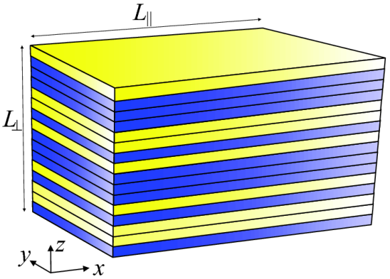
Figure 1: (Color online) Schematic of the layered Heisenberg magnet: It consistes of a random sequence of layers of two different ferromagnetic materials.Mohan et al. (2010)

Its Hamiltonian, a classical Heisenberg model on a three-dimensional lattice of perpendicular size $L_{\perp}$ (in $z$ direction) and in-plane size $L_{\parallel}$ (in the $x$ and $y$ directions) is given by

$$H=-\sum_{\mathbf{r}}J^{\parallel}_{z}\,(\mathbf{S}_{\mathbf{r}}\cdot\mathbf{S}_{\mathbf{r}+\hat{\mathbf{x}}}+\mathbf{S}_{\mathbf{r}}\cdot\mathbf{S}_{\mathbf{r}+\hat{\mathbf{y}}})-\sum_{\mathbf{r}}J^{\perp}_{z}\,\mathbf{S}_{\mathbf{r}}\cdot\mathbf{S}_{\mathbf{r}+\hat{\mathbf{z}}}.$$ (1)

Here, $\mathbf{S}_{\mathbf{r}}$ is a three-component unit vector on lattice site $\mathbf{r}$, and $\hat{\mathbf{x}}$, $\hat{\mathbf{y}}$, and $\hat{\mathbf{z}}$ are the unit vectors in the coordinate directions. The interactions within the layers, $J^{\parallel}_{z}$, and between the layers, $J^{\perp}_{z}$, are both positive and independent random functions of the perpendicular coordinate $z$.

In the following, we take all $J^{\perp}_{z}$ to be identical, $J^{\perp}_{z}\equiv J^{\perp}$, while the $J^{\parallel}_{z}$ are drawn from a binary probability distribution

$$P(J^{\parallel})=(1-p)\,\delta(J^{\parallel}-J_{u})+p\,\delta(J^{\parallel}-J_{l})$$ (2)

with $J_{u}>J_{l}$. Here, $p$ is the concentration of the “weak” layers while $1-p$ is the concentration of the “strong” layers.

The qualitative behavior of the model (1) is easily explained (see Fig. 2). At sufficiently high temperatures, the model is in a conventional paramagnetic (strongly disordered) phase. Below a temperature $T_{u}$ (the transition temperature of a hypothetical system having $J^{\parallel}_{z}\equiv J_{u}$ for all $z$) but above the actual critical temperature $T_{c}$, rare thick slabs of strong layers develop local order while the bulk system is still nonmagnetic. This is the paramagnetic (weakly disordered) Griffiths phase (or Griffiths region). In the ferromagnetic (weakly ordered) Griffiths phase, located between $T_{c}$ and a temperature $T_{l}$ (the transition temperature of a hypothetical system having $J^{\parallel}_{z}\equiv J_{l}$ for all $z$), bulk magnetism coexists with rare nonmagnetic slabs. Finally, below $T_{l}$, all slabs are locally ferromagnetic and the system is in a conventional ferromagnetic (strongly ordered) phase.

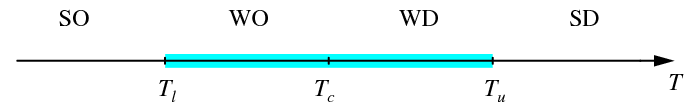
Figure 2: (Color online) Schematic phase diagram of the randomly layered Heisenberg magnet (1). SD and SO denote the conventional strongly disordered and strongly ordered phases, respectively. WD and WO are the weakly disordered and ordered Griffiths phases. $T_{c}$ is the critical temperature while $T_{u}$ and $T_{l}$ mark the boundaries of the Griffiths phase .

In Ref. Mohan et al., 2010, the behavior in both Griffiths phases and at criticality has been derived within a strong-disorder renormalization group calculation. Here, we simply motivate and summarize the results. The probability of finding a slab of $L_{RR}$ consecutive strong layers is given by simple combinatorics; it reads $w(L_{RR})\sim(1-p)^{L_{RR}}=e^{-\tilde{p}L_{RR}}$ with $\tilde{p}=-\ln(1-p)$. Each such slab is equivalent to a two-dimensional Heisenberg model with an effective interaction $L_{RR}J_{u}$. Because the two-dimensional Heisenberg model is exactly at its lower critical dimension, the renormalized distance from criticality, $\epsilon$, of such a slab decreases exponentially with its thickness, $\epsilon(L_{RR})\sim e^{-bL_{RR}}$.Vojta (2006); Vojta and Schmalian (2005) Combining the two exponentials gives a power-law probability density of locally ordered slabs,

$$\rho(\epsilon)\sim\epsilon^{\tilde{p}/b-1}=\epsilon^{1/z-1}$$ (3)

where the second equality defines the conventionally used dynamical exponent, $z$. It increases with decreasing temperature throughout the Griffiths phase and diverges as $z\sim 1/|T-T_{c}|$ at the actual critical point.

Many important observables follow from appropriate integrals of the density of states (3). The susceptibility can be estimated by $\chi\sim\int d\epsilon\,\rho(\epsilon)/\epsilon$. In an infinite system, the lower bound of the integral is 0; therefore, the susceptibility diverges in the entire temperature region where $z>1$. A finite system size $L_{\parallel}$ in the in-plane directions introduces a nonzero lower bound $\epsilon_{\rm min}\sim L_{\parallel}^{-2}$. Thus, for $z>1$, the susceptibility in the weakly disordered Griffiths phase diverges as

$$\chi(L_{\parallel})\sim L_{\parallel}^{2-2/z}$$ (4)

and in the weakly ordered Griffiths phase, it diverges as

$$\chi(L_{\parallel})\sim L_{\parallel}^{2+2/z}.$$ (5)

The strong-disorder renormalization group Mohan et al. (2010) confirms these simple estimates and gives $\chi\sim L_{\parallel}^{2}[\ln{(L_{\parallel}/a)}]^{2\phi-1/\psi}$ at criticality where $\phi=(1+\sqrt{5})/2$ and $\psi=1/2$ are critical exponents of the infinite randomness critical point.

The spin-wave stiffness $\rho_{s}$ is defined by the work needed to twist the spins of two opposite boundaries by a relative angle $\theta$. Specifically, in the limit of small $\theta$ and large system size, the free-energy density $f$ depends on $\theta$ as

$$f(\theta)-f(0)=\frac{1}{2}\rho_{s}\left(\frac{\theta}{L}\right)^{2}.$$ (6)

Because the randomly layered Heisenberg model is anisotropic, we need to distinguish the parallel spin-wave stiffness $\rho_{s}^{\parallel}$ from the perpendicular spin-wave stiffness $\rho_{s}^{\perp}$. To calculate the parallel spin-wave stiffness, we apply boundary conditions at $x=0$ and $x=L_{\parallel}$ and set $L=L_{\parallel}$ in Eq. (6) whereas the boundary conditions are applied at $z=0$ and $z=L_{\perp}$ to calculate the perpendicular spin-wave stiffness with $L=L_{\perp}$ in Eq. (6).

Let us first discuss the parallel stiffness. In this case, the free energy difference $f(\theta)-f(0)$ is simply the sum over all layers participating in the long-range order (each having the same twisted boundary conditions). Thus, $\rho_{s}^{\parallel}$ is nonzero everywhere in the ordered phase. The strong-disorder renormalization group approach Mohan et al. (2010) predicts

$$\rho_{s}^{\parallel}\sim m\sim|T-T_{c}|^{\beta}~{}~{}~{}~{}~{}~{}~{}~{}~{}~{}~{}~{}~{}~{}(T<T_{c})$$ (7)

where $\beta=(3-\sqrt{5})/2$ is the order parameter exponent of the infinite randomness critical point. The parallel stiffness behaves like the total magnetization $m=|\sum_{\mathbf{r}}{\langle\mathbf{S_{r}}\rangle}|/(L_{\perp}L_{\parallel}^{2})$, because both renormalize additively under the strong-disorder renormalization-group theory.Mohan et al. (2010)

If the twist $\theta$ is applied between the bottom ($z=0$) and the top ($z=L_{\perp}$) layers, the local twists between consecutive layers will vary from layer to layer. Minimizing $f(\theta)-f(0)$ leads to $\rho_{s}^{\perp}\sim\langle 1/J_{eff}^{\perp}\rangle^{-1}$ where $J_{eff}^{\perp}$ are the effective couplings between the rare regions. Within the strong-disorder renormalization group approach, the distribution of the $J_{eff}^{\perp}$ follows a power law $p(J_{eff}^{\perp})\sim(J_{eff}^{\perp})^{1/z-1}$. Thus, $\rho_{s}^{\perp}=0$ in part of the ordered Griffiths phase. It only becomes nonzero once $z$ falls below $1$ at a temperature $T_{s}<T_{c}$. Between $T_{c}$ and $T_{s}$, the system displays anomalous elasticity. Here, the free energy due to the twist scales with $f(\theta)-f(0)\sim L_{\perp}^{-1-z}$. Thus, the perpendicular stiffness formally vanishes as $\rho_{s}^{\perp}\sim L_{\perp}^{1-z}$ with increasing $L_{\perp}$.

To study the dynamical critical behavior, a phenomenological dynamics is added to the randomly layered Heisenberg model. The simplest case is a purely relaxational dynamics corresponding to model $A$ in the classification of Hohenberg and Halperin.Hohenberg and Halperin (1977)

The dynamic behavior can be characterized by the average time autocorrelation function

$$C(t)=\frac{1}{L_{\perp}L_{\parallel}^{2}}\int{d^{3}r\langle\mathbf{S}_{\mathbf{r}}(t)\mathbf{S}_{\mathbf{r}}(0)\rangle},$$ (8)

where $\mathbf{S_{r}}(t)$ is the value of the spin at position $\mathbf{r}$ and time $t$.

The behavior of $C(t)$ in the weakly disordered Griffiths phase can be easily estimated. The correlation time of a single locally ordered slab is proportional to $1/\epsilon$.Mohan et al. (2010) Summing over all slabs using the density of states (3) then gives

$$C(t)\sim\int{d\epsilon\rho(\epsilon)e^{-\epsilon t}}\sim t^{-1/z}.$$ (9)

The strong disorder renormalization group calculation Mohan et al. (2010) confirms this estimate. Moreover, at criticality, when $z\to\infty$, it gives an even slower logarithmic behavior

$$C(t)\sim[\ln(t/t_{0})]^{\phi-1/\psi}.$$ (10)

where $t_{0}$ is a microscopic length scale.

III Monte-Carlo simulations

III.1 Overview

In this section we report results of Monte-Carlo simulations of the randomly layered Heisenberg magnet. Because the phase transition in this system is dominated by the rare regions, sufficiently large system sizes are required in order to get reliable results. We have simulated system sizes ranging from $L_{\perp}=90$ to $800$ and $L_{\parallel}=10$ to $400$. We have chosen $J_{u}=1$ and $J_{l}=0.25$ in Eq. (2). All the simulations have been performed for disorder concentrations $p=0.8$. With these parameter choices, the Griffiths region ranges from $T_{l}\approx 0.63$ to $T_{u}\approx 1.443$. For optimal performance, we have used large numbers of disorder realizations, ranging from $100$ to $7200$, depending on the system size. While studying the thermodynamics, we have used the efficient Wolff cluster algorithm Wolff (1989) to eliminate critical slowing down. We have equilibrated every run by 100 Monte-Carlo sweeps, and we have used another 100 sweeps for measurements. To investigate the critical dynamics, we have equilibrated the system using the Wolff algorithm but then propagated the system in time by means of the Metropolis algorithm Metropolis et al. (1953) which implements model $A$ dynamics.

III.2 Thermodynamics

To test the finite-size behavior (4, 5) of the susceptibility, one needs to consider samples having sizes $L_{\perp}\gg L_{\parallel}$ such that $L_{\perp}$ is effectively infinite. We have used system sizes $L_{\perp}=800$ and $L_{\parallel}=10$ to $90$. Figure 3 shows the susceptibility $\chi$ as a function of $L_{\parallel}$ for several temperatures in the Griffiths region between $T_{l}=0.63$ and $T_{u}\approx 1.443$. In agreement with the theoretical predictions (4) and (5), $\chi$ follows a nonuniversal power law in $L_{\parallel}$ with a temperature-dependent exponent. Simulations for many more temperature values, in the range $T\approx 0.76-1.2$, yield analogous results.

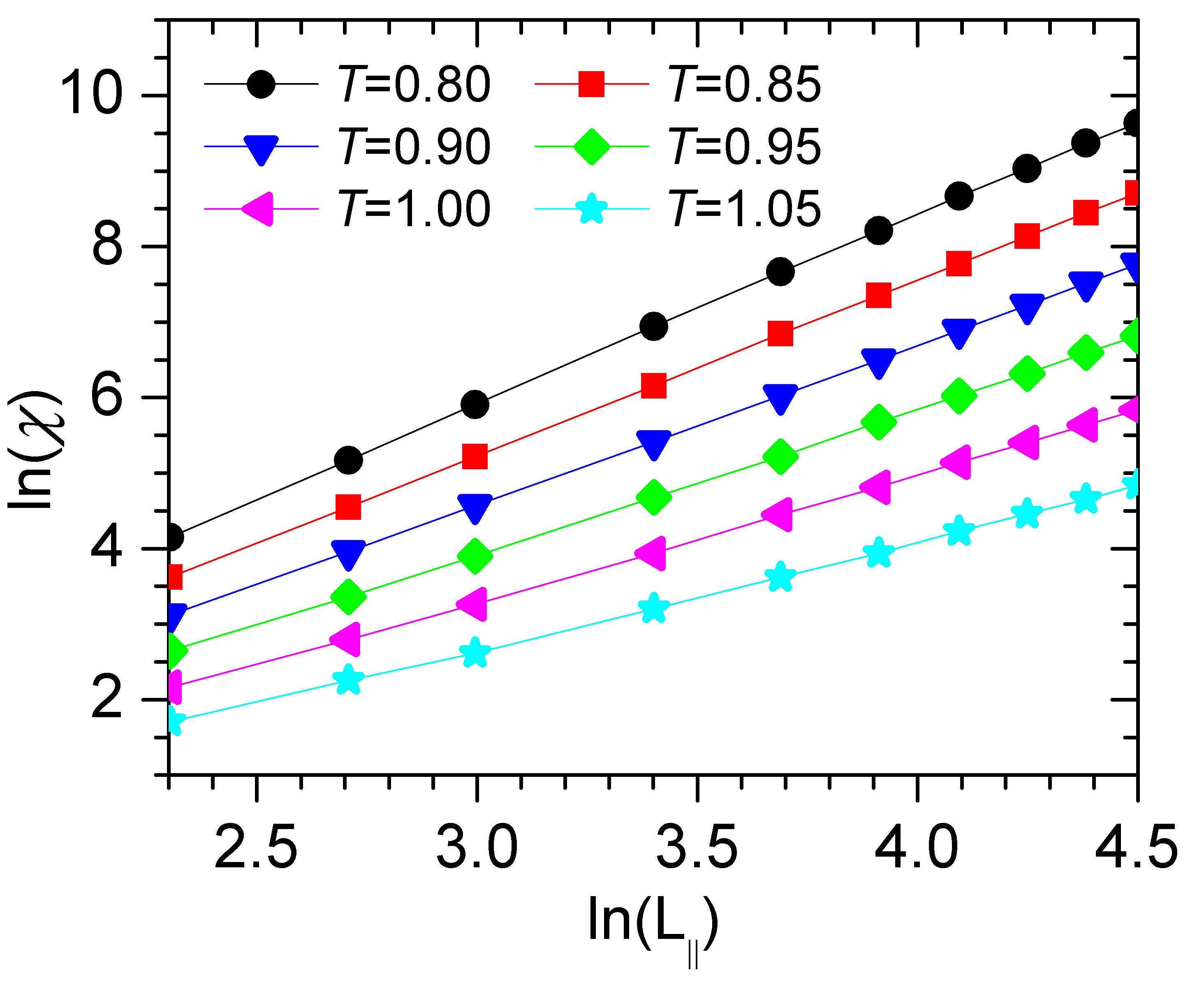
Figure 3: (Color online) Susceptibility $\chi$ as a function of in-plane system size $L_{\parallel}$ for several temperatures in the Griffiths region. The perpendicular size is $L_{\perp}=800$; the data are averages over 300 disorder configurations. The solid lines are fits to the power laws (4, 5).

The values of the exponent $z$ extracted from fits to (4, 5) are shown in Fig. 4 for the paramagnetic and ferromagnetic sides of the Griffiths region. $z$ can be fitted to the predicted power law $z\sim 1/|T-T_{c}|$, as discussed after (3), giving the estimate $T_{c}\approx 0.933$.

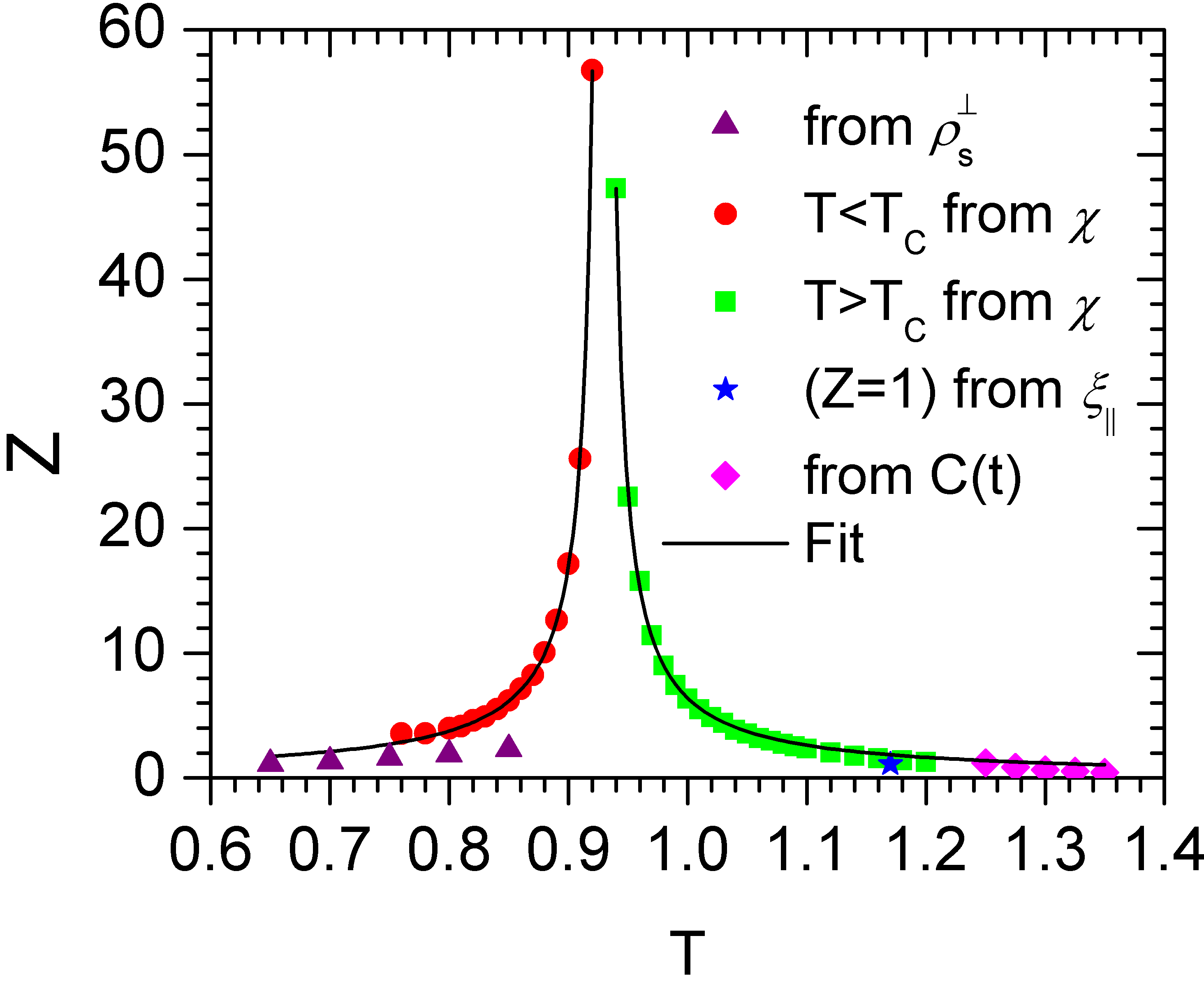
Figure 4: (Color online) Griffiths dynamical exponent $z$ vs temperature. The data are extracted from the perpendicular stiffness data in Fig. 6b, the susceptibility data in Fig. 3, the parallel correlation length data in Fig. 5 and the autocorrelation function data in Fig. 7. The solid lines are a power-law fit of $z$ (extracted from Fig. 3) to (4) and (5).

For a deeper understanding of the thermodynamic critical phenomena of the layered Heisenberg model, we have also studied the behavior of the in-plane correlation lengths in Griffiths phase. Figure 5 shows the scaled correlation length $\xi_{\parallel}/L_{\parallel}$ as a function of temperature for different values of $L_{\parallel}$. Surprisingly, the curves cross at a temperature, $T\approx 1.17$, significantly higher than $T_{c}\approx 0.93$. This implies that the average in-plane correlation length diverges in part of the disordered phase.

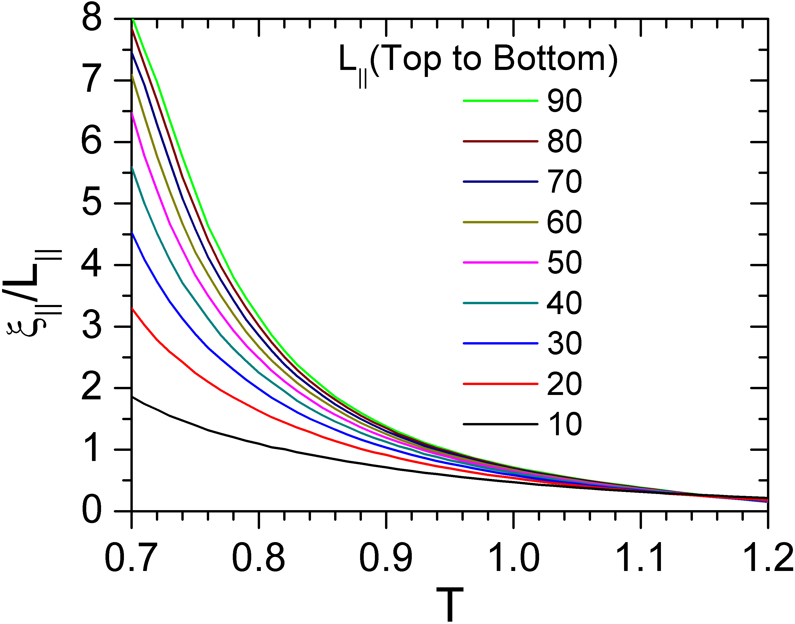
Figure 5: (Color online) Scaled in-plane correlation length $\xi_{\parallel}/L_{\parallel}$ as a function of temperature $T$ for several in-plane system sizes $L_{\parallel}$ in the Griffiths region. The perpendicular size is $L_{\perp}=800$; the data are averaged over 300 disorder configurations.

To understand this behavior, we estimate the rare region contribution to the averaged in-plane correlation length. It can be calculated by integrating over the density of states (3) as

$$\xi_{\parallel}^{2}\sim\int_{0}^{\epsilon_{0}}{d\epsilon\rho(\epsilon)\xi_{\parallel}^{2}(\epsilon)}\sim\int_{0}^{\epsilon_{0}}{d\epsilon\epsilon^{1/z-1}\frac{1}{\epsilon}}$$ (11)

where $\xi_{\parallel}^{2}(\epsilon)\sim 1/\epsilon$ is the dependence of the in-plane correlation length of a single region Mohan et al. (2010); Bray (1988) on the renormalized distance $\epsilon$ from criticality. Note that we average $\xi_{\parallel}^{2}$ instead of $\xi_{\parallel}$ because that is what numerically happens in the second moment method which defines $\xi_{\parallel}^{2}$ via

$$\xi_{\parallel}^{2}=\frac{\sum_{\mathbf{r}}{C(\mathbf{r})\mathbf{r}^{2}}}{\sum_{\mathbf{r}}{C(\mathbf{r})}}$$ (12)

with $C(\mathbf{r})$ being the spatial correlation function. The integral in (11) diverges for $z>1$ and converges for $z<1$. The in-plane correlation length therefore diverges already in the disordered Griffiths phase at the temperature at which the Griffiths dynamical exponent is $z=1$. From Fig. 5 we estimate this temperature to be $T\approx 1.17$. As can be seen in Fig. 4, this value is in good agreement with the result extracted from the finite size behavior of $\chi$.

We now turn to the spin-wave stiffness. Calculating the stiffness by actually carrying out simulations with twisted boundary conditions is not very efficient. However, the stiffness can be rewritten in terms of expectation values calculated in a conventional run with periodic boundary conditions. The resulting formula which is a generalization of that used by Caffarel et al Caffarel et al. (1994) reads

$$\begin{gathered}\rho_{s}^{\perp}=\left\langle\sum_{\langle\mathbf{r},\mathbf{r}^{\prime}\rangle}J_{\mathbf{r},\mathbf{r}^{\prime}}\left[\mathbf{S}_{\mathbf{r}}\cdot\mathbf{S}_{\mathbf{r}^{\prime}}-(\mathbf{S}_{\mathbf{r}}\cdot\hat{\mathbf{a}})(\mathbf{S}_{\mathbf{r}^{\prime}}\cdot\hat{\mathbf{a}})\right](z-z^{\prime})^{2}\right\rangle\\ -\frac{1}{T}\left\langle\left(\sum_{\langle\mathbf{r},\mathbf{r}^{\prime}\rangle}J_{\mathbf{r},\mathbf{r}^{\prime}}\left[(\mathbf{S}_{\mathbf{r}}\times\mathbf{S}_{\mathbf{r}^{\prime}})\cdot\hat{\mathbf{a}}\right](z-z^{\prime})\right)^{2}\right\rangle.\end{gathered}$$ (13)

Here, $\hat{\mathbf{a}}$ can be any unit vector perpendicular to the total magnetization $\mathbf{m}$. For $\rho_{s}^{\parallel}$, $(z-z^{\prime})$ has to be replaced by $(x-x^{\prime})$. This formula is derived in appendix A.

Figure 6a shows the results for the perpendicular and parallel stiffnesses of our randomly layered Heisenberg model. We have used a system of size $L_{\perp}=100$ and $L_{\parallel}=400$. The figure shows that the two stiffness indeed behave very differently. The parallel stiffness $\rho_{s}^{\parallel}$ vanishes at $T\approx 0.9-0.95$ in good agreement with our earlier estimate of $T_{c}\approx 0.93$. In contrast, the perpendicular stiffness vanishes at a much lower temperature $T\approx 0.7$. Thus, in the range between $T\approx 0.7$ and $T_{c}$, the system displays anomalous elasticity, as predicted. (Note: The slight rounding of both $\rho_{s}^{\parallel}$ and $\rho_{s}^{\perp}$ can be attributed to finite-size effects.)

The results of the perpendicular spin-wave stiffness $\rho_{s}^{\perp}$ are analyzed in more detail in Fig. 6b for perpendicular sizes $L_{\perp}=15-40$. We have used a parallel size $L_{\parallel}=400$ and a temperature range $T=0.65-0.85$ where the data are averaged over 1000 disorder configurations. The plot shows a non-universal power-law dependence of $\rho_{s}^{\perp}$ on $L_{\perp}$ which agrees with the prediction

$$\rho_{s}^{\perp}\sim L_{\perp}^{1-z}.$$ (14)

The dynamical exponents $z$ extracted from fits of $\rho_{s}^{\perp}$ to (14) are also shown in Fig. 4. While they roughly agree with the values extracted from $\chi$, the agreement is not very good. We believe this is due to the rather small $L_{\perp}$ values used.

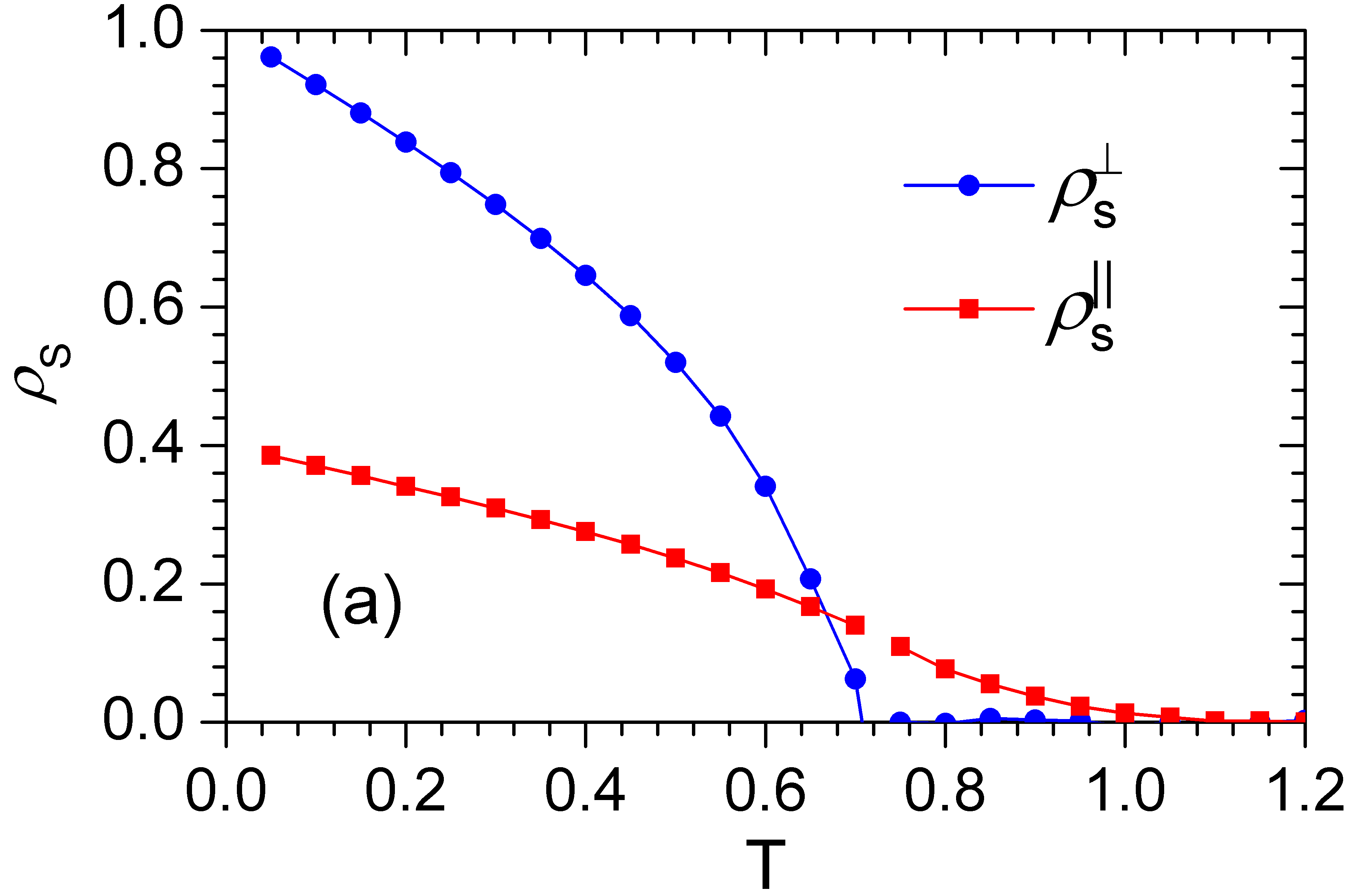
(a)

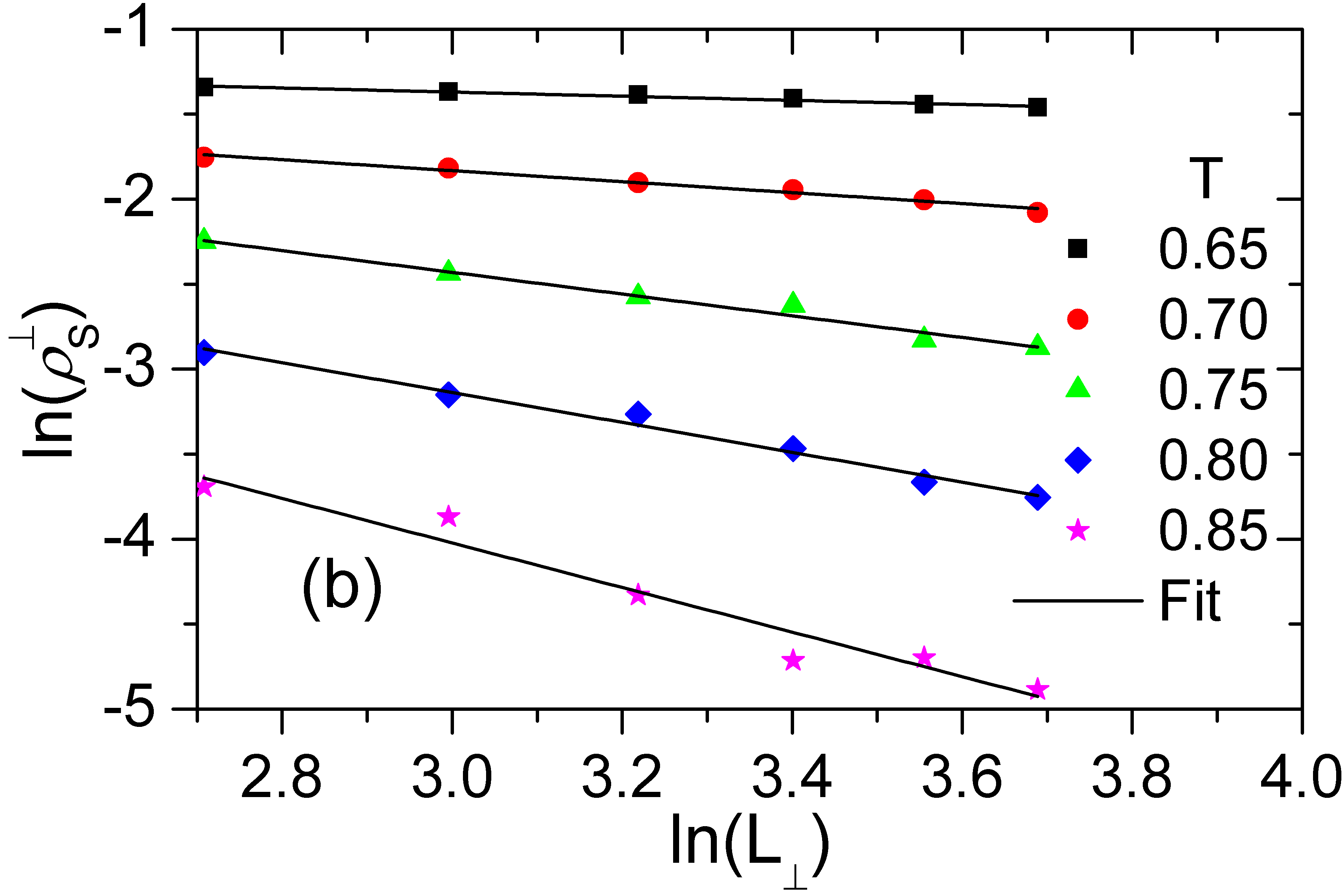
(b)

Figure 6: (Color online) a: Perpendicular and parallel spin-wave stiffnesses ($\rho_{s}^{\perp}$ and $\rho_{s}^{\parallel}$, respectively) as functions of temperature $T$ for system with sizes $L_{\perp}=100$ and $L_{\parallel}=400$. The data are averaged over 100 disorder configurations. b: Perpendicular spin-wave stiffness as a function of $L_{\perp}$ for temperatures in the weakly ordered Griffiths phase and $L_{\parallel}=400$. The data are averaged over 1000 disorder configurations. The solid lines are fits to (14).

III.3 Critical dynamics

To investigate the behavior of the autocorrelation function $C(t)$ in the weakly disordered Griffiths phase, we have used system sizes $L_{\perp}=400$ and $L_{\parallel}=100$ and temperatures from $T=1.25$ to $1.35$. From figure 7, one can see that the long-time behavior of $C(t)$ in the Griffiths phase follows a non-universal power law which is in agreement with the prediction (9). Fits of the data to (9) can be used to obtain yet another estimate of the dynamical exponent $z$. The resulting values are shown in Fig. 4, they are in good agreement with those extracted from $\chi$.

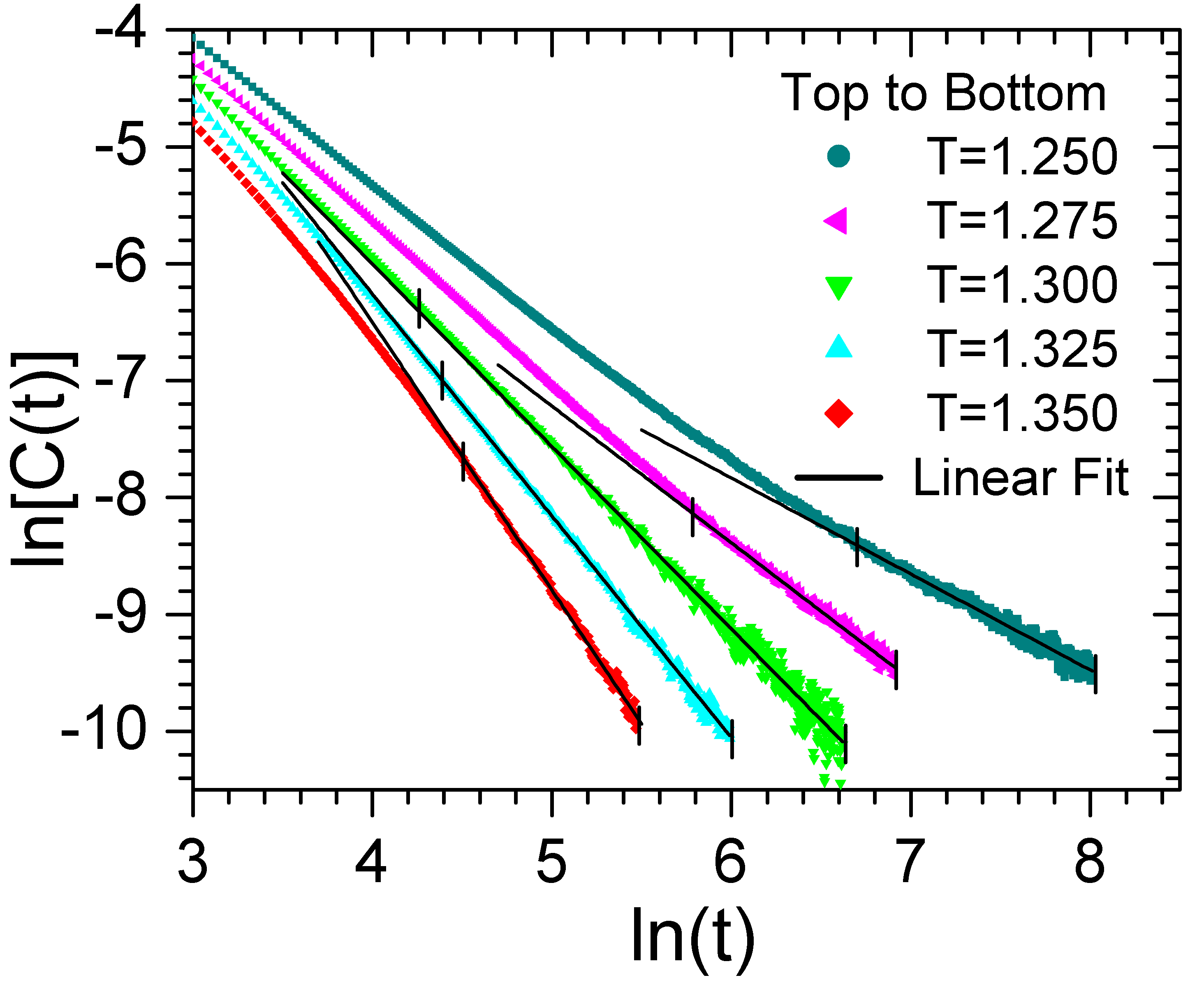
Figure 7: (Color online) Time autocorrelation function $C(t)$ for temperatures from $T=1.25$ to $1.35$ (within the Griffiths phase). The system sizes are $L_{\perp}=400$ and $L_{\parallel}=100$. The data are averaged over $1720-7200$ disorder configurations. The solid lines are fits to the power-law prediction (9) (with the fit range marked).

Figure 8 shows the behavior of $C(t)$ near criticality plotted such that the expected logarithmic time-dependence (10) gives a straight line. We have used system sizes $L_{\perp}=400$ and $L_{\parallel}=230$ and temperatures from $T=0.86$ to $0.91$. We find that $C(t)$ indeed follows the prediction at an estimated $T_{c}\approx 0.895$. This estimate agrees reasonably well with that stemming from the finite-size behavior of $\chi$. We attribute the remaining difference to the finite-size effects and (in case of $C(t)$) finite-time effects.

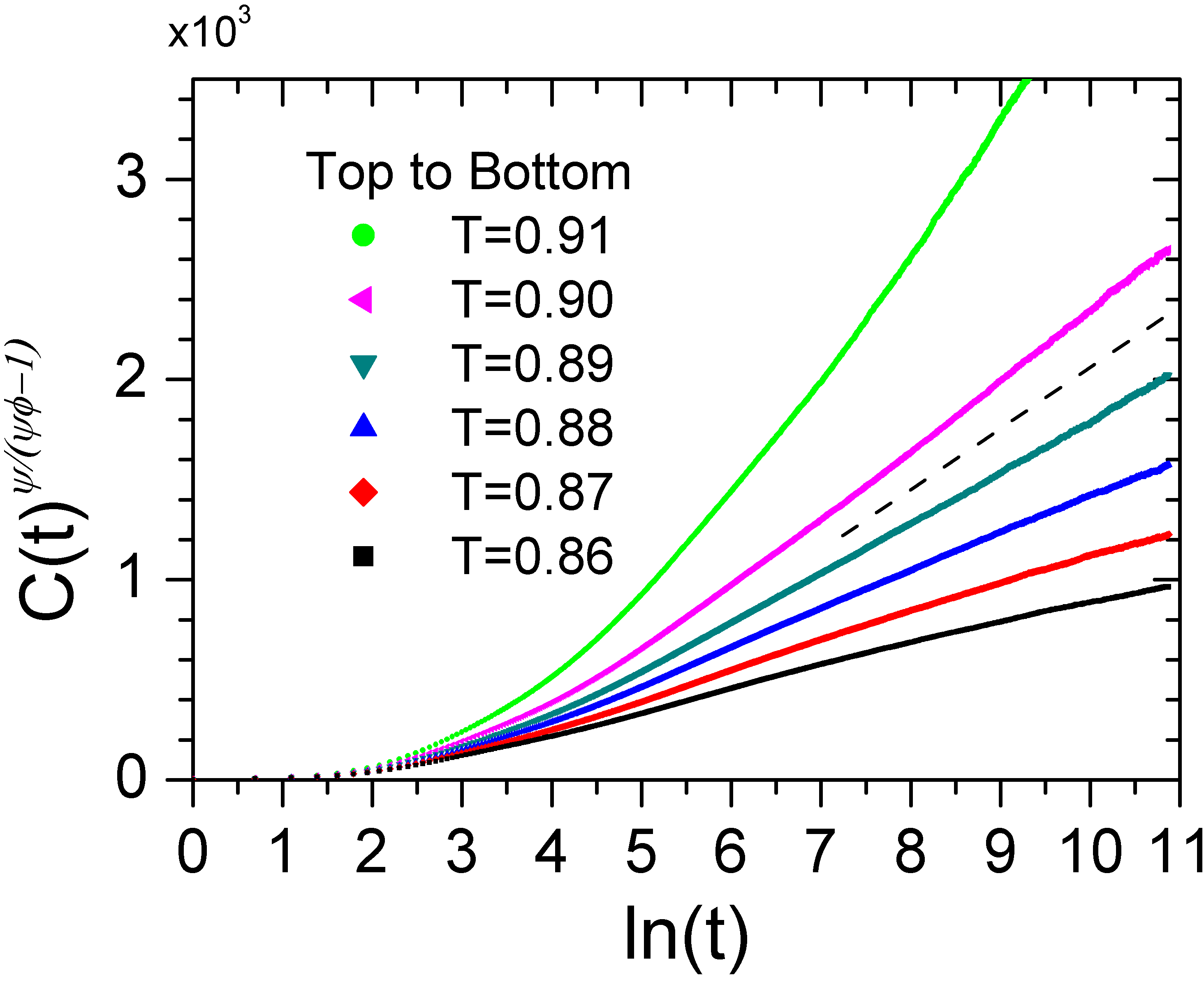
Figure 8: (Color online) Time autocorrelation function $C(t)$ for temperatures from $T=0.86$ to $0.91$ (near criticality). The system sizes are $L_{\perp}=400$ and $L_{\parallel}=230$. The data are averaged over 70 to 80 disorder configurations. The dashed line shows the logarithmic behavior (10) at the estimated critical temperature $T_{c}=0.895$.

IV Conclusions

To summarize, we have reported the results of large-scale Monte-Carlo simulations of the thermodynamics and dynamic behavior of a randomly layered Heisenberg model. Our results provide strong numerical evidence in support of the infinite-randomness scenario predicted within the strong-disorder renormalization group approach.Mohan et al. (2010) Morever, our data are compatible with the prediction that the randomly layered Heisenberg model is in the same universality class as the one-dimensional random transverse-field Ising model.

We would have liked to determine the complete set of critical exponents of the infinite-randomness critical point directly from the numerical data. To this end we have attempted to perform an anisotropic finite-size scaling analysis as in Refs. Pich et al., 1998 or Sknepnek et al., 2004. However, within the accessible range of system sizes of up to about $10^{7}$ sites, the corrections to the leading scaling behavior were so strong that we could not complete the analysis. This task thus remains for the future.

An important question left unanswered by the strong-disorder renormalization group approachMohan et al. (2010) is whether or not weakly or moderately disordered systems actually flow to the infinite-randomness critical point. The clean Heisenberg critical point is unstable against weak layered disorder because it violates the generalized Harris criterion $d_{r}\nu>2$ where $d_{r}=1$ is the number of random dimensions. Thus, weak layered randomness initially increases under renormalization. Our numerical parameter choices, $p=0.8$ and $J_{u}/J_{l}=4$ correspond to moderate disorder as the distribution is not particularly broad on a logarithmic scale. The fact that we do confirm infinte-randomness behavior for these parameters suggests that the infinite-randomness critical point may control the transition for any nonzero disorder strength. A numerical verification of this conjecture by simulating very weakly disordered systems would require even larger system sizes and is thus beyond our present computational capabilities.

Experimental verifications of infinite-randomness critical behavior and the accompanying power-law Griffiths singularities have been hard to come by, in particular in higher-dimensional systems. Only very recently, promising measurements have been reported Westerkamp et al. (2009); Ubaid-Kassis et al. (2010) of the quantum phase transitions in CePd_1-xRh_x and Ni_1-xV_x. The randomly layered Heisenberg magnet considered here provides an alternative realization of an infinite-randomness critical point. It may be more easily realizable in experiment because the critical point is classical, and samples can be produced by depositing random layers of two different ferromagnetic materials.

Magnetic multilayers with systematic variation of the critical temperature from layer to layer have already been produced,Marcellini et al. (2009) and our results would apply to random versions of these structures.

Appendix A Spin-wave stiffness in terms of spin correlation functions

Twisted boundary conditions, i.e., forcing the spins on one surface of the sample of size $L$ to make an angle of $\theta$ with those on the opposite surface, lead to a change in the free energy density $f$. It can be parametrized by

$$f(\theta)-f(0)=\frac{1}{2}\rho_{s}\left(\frac{\theta}{L}\right)^{2}.$$ (15)

which defines the spin-wave stiffness $\rho_{s}$.

For definiteness, assume we apply a twist of $\theta$ around the perpendicular axis between the top and bottom surfaces of the sample. We parametrize the Heisenberg spin as

$$\mathbf{S}_{\mathbf{r}}=\begin{pmatrix}\sin(\vartheta_{\mathbf{r}})\cos(\phi_{\mathbf{r}})\\ \sin(\vartheta_{\mathbf{r}})\sin(\phi_{\mathbf{r}})\\ \cos(\vartheta_{\mathbf{r}})\end{pmatrix}.$$ (16)

The boundary conditions then read $\phi_{\mathbf{r}}=0$ at the bottom $(z=0)$ surface and $\phi_{\mathbf{r}}=\theta$ at the top $(z=L_{\perp})$ surface. To eliminate the twisted boundary condition, we now perform the variable transformation

$$\psi_{\mathbf{r}}=\phi_{\mathbf{r}}-\theta\frac{z_{\mathbf{r}}}{L_{\perp}}$$ (17)

which gives new boundary conditions of $\psi_{\mathbf{r}}=0$ at both $z_{\mathbf{r}}=0$ and $z_{\mathbf{r}}=L_{\perp}$.

Substituting the variable transformation in the Heisenberg Hamiltonian (1), we obtain

$$\begin{split}H=&-\sum_{\langle\mathbf{r},\mathbf{r}^{\prime}\rangle}{J_{\mathbf{r},\mathbf{r}^{\prime}}}\bigg{\{}\sin(\vartheta_{\mathbf{r}})\ \sin(\vartheta_{\mathbf{r}^{\prime}})\\ &\cos{\bigg{(}\psi_{\mathbf{r}}-\psi_{\mathbf{r}^{\prime}}+\frac{\theta}{L_{\perp}}(z-z^{\prime})\bigg{)}}+\cos(\vartheta_{\mathbf{r}})\ \cos(\vartheta_{\mathbf{r}^{\prime}})\bigg{\}}\\ \end{split}$$ (18)

where the twist is “distributed” over the volume. Thus, the twist angle $\theta$ now appears as a parameter of the Hamiltonian. We can use standard methods to reformulate the second derivative of the free energy $F$ as

$$\frac{\partial^{2}F}{\partial\theta^{2}}=\frac{1}{T}\left\langle\frac{\partial H}{\partial\theta}\right\rangle^{2}+\left\langle\frac{\partial^{2}H}{\partial\theta^{2}}\right\rangle\\ -\frac{1}{T}\left\langle\left(\frac{\partial H}{\partial\theta}\right)^{2}\right\rangle\\$$ (19)

where the first term on the right hand side vanishes due to symmetry. Evaluating the derivatives of $H$ for the Hamiltonian (18) gives the spin-wave stiffness $\rho_{s}=L^{2}({\partial^{2}f}/{\partial\theta^{2}})\big{|}_{\theta=0}$ as

$$\begin{gathered}\rho_{s}^{\perp}=\left\langle\sum_{\langle\mathbf{r},\mathbf{r}^{\prime}\rangle}J_{\mathbf{r},\mathbf{r}^{\prime}}\left[\mathbf{S}_{\mathbf{r}}\cdot\mathbf{S}_{\mathbf{r}^{\prime}}-(\mathbf{S}_{\mathbf{r}}\cdot\hat{\mathbf{k}})(\mathbf{S}_{\mathbf{r}^{\prime}}\cdot\hat{\mathbf{k}})\right](z-z^{\prime})^{2}\right\rangle\\ -\frac{1}{T}\left\langle\left(\sum_{\langle\mathbf{r},\mathbf{r}^{\prime}\rangle}J_{\mathbf{r},\mathbf{r}^{\prime}}\left[(\mathbf{S}_{\mathbf{r}}\times\mathbf{S}_{\mathbf{r}^{\prime}})\cdot\hat{\mathbf{k}}\right](z-z^{\prime})\right)^{2}\right\rangle.\end{gathered}$$ (20)

Here, $\hat{\mathbf{k}}$ is the unit vector in the $z$-direction. The same equation was derived in Ref. Caffarel et al., 1994 for the $XY$ case. Equation 20 needs to be evaluated with fixed boundary conditions at the top and bottom layeres. Applying this formula to simulations with periodic boundary conditions leads to incorrect results in the Heisenberg case (even though it works in $XY$ case). The reason is that Eq. (20) is sensitive to twist in the $XY$ plane only.

In the Heisenberg case this can be fixed by aligning the imaginary twist axis with a direction $\hat{\mathbf{a}}$ perpendicular to the total magnetization in each Monte-Carlo measurement. We use $\hat{\mathbf{a}}=(\mathbf{m}\times\hat{\mathbf{k}})/|\mathbf{m}\times\hat{\mathbf{k}}|$. The resulting formula for the spin-wave stiffness can be used efficiently by Monte-Carlo simulations with periodic boundary conditions. It reads

$$\begin{gathered}\rho_{s}^{\perp}=\left\langle\sum_{\langle\mathbf{r},\mathbf{r}^{\prime}\rangle}J_{\mathbf{r},\mathbf{r}^{\prime}}\left[\mathbf{S}_{\mathbf{r}}\cdot\mathbf{S}_{\mathbf{r}^{\prime}}-(\mathbf{S}_{\mathbf{r}}\cdot\hat{\mathbf{a}})(\mathbf{S}_{\mathbf{r}^{\prime}}\cdot\hat{\mathbf{a}})\right](z-z^{\prime})^{2}\right\rangle\\ -\frac{1}{T}\left\langle\left(\sum_{\langle\mathbf{r},\mathbf{r}^{\prime}\rangle}J_{\mathbf{r},\mathbf{r}^{\prime}}\left[(\mathbf{S}_{\mathbf{r}}\times\mathbf{S}_{\mathbf{r}^{\prime}})\cdot\hat{\mathbf{a}}\right](z-z^{\prime})\right)^{2}\right\rangle.\end{gathered}$$ (21)

We have tested that this equation reproduces the results obtained directly from Eq. (15).

References

- Harris (1974) A. B. Harris, J. Phys. C 7, 1671 (1974).
- Thill and Huse (1995) M. Thill and D. A. Huse, Physica A 214, 321 (1995).
- Guo et al. (1996) M. Guo, R. N. Bhatt, and D. A. Huse, Phys. Rev. B 54, 3336 (1996).
- Rieger and Young (1996) H. Rieger and A. P. Young, Phys. Rev. B 54, 3328 (1996).
- Fisher (1992) D. S. Fisher, Phys. Rev. Lett. 69, 534 (1992).
- Fisher (1995) D. S. Fisher, Phys. Rev. B 51, 6411 (1995).
- Vojta (2003a) T. Vojta, Phys. Rev. Lett. 90, 107202 (2003a).
- Hoyos and Vojta (2008) J. A. Hoyos and T. Vojta, Phys. Rev. Lett. 100, 240601 (2008).
- Vojta (2006) T. Vojta, J. Phys. A 39, R143 (2006).
- Vojta (2010) T. Vojta, J. Low Temp. Phys. 161, 299 (2010).
- McCoy and Wu (1968a) B. M. McCoy and T. T. Wu, Phys. Rev. Lett. 21, 549 (1968a).
- McCoy and Wu (1968b) B. M. McCoy and T. T. Wu, Phys. Rev. 176, 631 (1968b).
- McCoy and Wu (1969) B. M. McCoy and T. T. Wu, Phys. Rev. 188, 982 (1969).
- McCoy (1969) B. M. McCoy, Phys. Rev. Lett. 23, 383 (1969).
- Vojta (2003b) T. Vojta, J. Phys. A 36, 10921 (2003b).
- Sknepnek and Vojta (2004) R. Sknepnek and T. Vojta, Phys. Rev. B 69, 174410 (2004).
- Mohan et al. (2010) P. Mohan, R. Narayanan, and T. Vojta, Phys. Rev. B 81, 144407 (2010).
- Vojta and Schmalian (2005) T. Vojta and J. Schmalian, Phys. Rev. B 72, 045438 (2005).
- Hohenberg and Halperin (1977) P. C. Hohenberg and B. I. Halperin, Rev. Mod. Phys. 49, 435 (1977).
- Wolff (1989) U. Wolff, Phys. Rev. Lett. 62, 361 (1989).
- Metropolis et al. (1953) N. Metropolis, A. Rosenbluth, M. Rosenbluth, and A. Teller, J. Chem. Phys. 21, 1087 (1953).
- Bray (1988) A. J. Bray, Phys. Rev. Lett. 60, 720 (1988).
- Caffarel et al. (1994) M. Caffarel, P. Azaria, B. Delamotte, and D. Mouhanna, Europhys Lett. 26, 493 (1994).
- Pich et al. (1998) C. Pich, A. P. Young, H. Rieger, and N. Kawashima, Phys. Rev. Lett. 81, 5916 (1998).
- Sknepnek et al. (2004) R. Sknepnek, T. Vojta, and M. Vojta, Phys. Rev. Lett. 93, 097201 (2004).
- Westerkamp et al. (2009) T. Westerkamp, M. Deppe, R. Küchler, M. Brando, C. Geibel, P. Gegenwart, A. P. Pikul, and F. Steglich, Phys. Rev. Lett. 102, 206404 (2009).
- Ubaid-Kassis et al. (2010) S. Ubaid-Kassis, T. Vojta, and A. Schroeder, Phys. Rev. Lett. 104, 066402 (2010).
- Marcellini et al. (2009) M. Marcellini, M. Pärnaste, B. Hjörvarsson, and M. Wolff, Phys. Rev. B 79, 144426 (2009).