Dynamics of cooperativity in chemical sensing among cell-surface receptors

Abstract

Cooperative interactions among sensory receptors provide a general mechanism to increase the sensitivity of signal transduction. In particular, bacterial chemotaxis receptors interact cooperatively to produce an ultrasensitive response to chemoeffector concentrations. However, cooperativity between receptors in large macromolecular complexes is necessarily based on local interactions and consequently is fundamentally connected to slowing of receptor conformational dynamics, which increases intrinsic noise. Therefore, it is not clear whether or under what conditions cooperativity actually increases the precision of the concentration measurement. We explictly calculate the signal-to-noise ratio (SNR) for sensing a concentration change using a simple, Ising-type model of receptor-receptor interactions, generalized via scaling arguments, and find that the optimal SNR is always achieved by independent receptors.

In biological networks, cooperative interactions among components can sharpen input-output relations, increasing gain and enabling switch-like responses. The best-known example is the cooperative binding/release of oxygen by hemoglobin, which enables efficient transport of oxygen between the lungs and tissue. In sensory systems, a well-studied example of cooperativity is receptor-receptor coupling in Escherichia coli chemotaxis Sourjik and Berg (2002). For sensing systems, there is an obvious advantage of high gain to amplify weak signals Bray et al. (1998), particularly when combined with an adaptation system to broaden the dynamic range Hansen et al. (2008). This advantage of high gain from receptor-receptor interactions raises the question: why has receptor coupling not evolved in other chemical sensing systems, e.g. quorum sensing and eukaryotic chemotaxis?

If the function of a sensory network is to reliably detect weak signals, then processing of the signal is only half the story. The other half is the suppression of noise and for weak signals the signal-to-noise ratio (SNR) generally governs information transmission and sensory performance sup . Cellular signal transduction must contend with both noisy inputs (extrinsic noise), as well as the noise generated internally by the signal transduction system itself (intrinsic noise). While the presence of signaling noise is well appreciated, the connection between cooperativity and noise has received less attention Berg et al. (2000); *ShibataFujimoto2004; Bialek and Setayeshgar (2008); *Aquino2011; *Hu2010. As we will show, receptor cooperativity and intrinsic signaling noise are inextricably linked via the statistical mechanics of receptors. The same cooperative interactions that give rise to enhanced sensitivity necessarily both amplify fluctuations and slow the rate of receptor-conformational switching, limiting both the response time and the ability of the system to reduce intrinsic noise by time-averaging. Due to these tradeoffs, it is unclear when or whether receptor cooperativity actually increases sensory performance.

The prevailing view of bacterial chemoreceptor operation is that signal amplification from receptor cooperativity enables the chemotaxis network to reliably detect shallow gradients with exquisite sensitivity. In this Letter, we challenge this viewpoint by evaluating the strategy of using receptor cooperativity to enhance weak signal detection in light of the tradeoffs between gain and intrinsic noise. Specifically, we calculate the SNR for a simple physical model of receptor-receptor interactions, a dynamical Ising-type model in which receptors have two conformational states, active and inactive, and neighboring receptors prefer to be in the same conformational state (a.k.a. conformational spread Bray et al. (1998)). The input to the network is the (changing) external ligand concentration and the output is the time-averaged total receptor activity. This two-state model is a good description of bacterial chemoreceptors, in which the active and inactive conformational states are named for their relative abilities to activate a downstream kinase Wadhams and Armitage (2004) and the output of the network is the CheY-P concentration, which is effectively the time-average of receptor activity over the phosphorylated lifetime of individual CheY-P molecules.

Importantly, our model is the first to both (i) incorporate the dynamics of receptor switching, which is key to understanding the reduction in noise by time-averaging and (ii) base cooperativity on local interactions. Unlike the dynamic MWC models used in previous work Bialek and Setayeshgar (2008); *Aquino2011, we invoke no unphysical action-at-a-distance that allows the entire receptor cluster to flip conformational states simultaneously. In fact, a recent study has provided direct evidence for local interactions underlying the ultrasensitive behavior of the bacterial motor Bai et al. (2010).

We consider a cell with a total of $N$ two-state receptors, which are divided into $m$ independent 1D chains each of length $n$, with nearest-neighbor Ising couplings inside each chain, given by the Hamiltonian

$$H=-J\sum_{\langle i,j\rangle}\sigma_{i}\sigma_{j}+\frac{1}{2}\sum_{i=1}^{n}f\sigma_{i},$$ (1)

where $\sigma_{i}=\pm 1$ represents the active/inactive receptor states, $\langle i,j\rangle$ denotes nearest neighbors, and

$$f=\Delta\epsilon+\log{\left(\frac{1+[\text{L}]/K^{\text{off}}}{1+[\text{L}]/K^{\text{on}}}\right)}$$ (2)

is the free-energy difference between active and inactive states, which is a function of the ligand concentration $[L]$, ligand dissociation constants $K^{\text{off}}$ and $K^{\text{on}}$, and the “offset energy” $\Delta\epsilon\equiv E_{\text{on}}-E_{\text{off}}$, which is the energy difference between active and inactive states in the absence of ligand Keymer et al. (2006)  .

When ligand binding/unbinding is much faster than receptor conformational switching, the stochastic dynamics of switching is governed by a kinetic Ising model, where the occupation probablity $p(\sigma_{1},\dots\sigma_{n};t)$ obeys the master equation

$$\frac{d}{dt}p(\sigma_{1},\dots\sigma_{n};t) = -\left(\sum_{i}k_{i}(\sigma_{i})\right)p(\sigma_{1},\dots\sigma_{n};t)$$

$$+\sum_{i}k_{i}(-\sigma_{i})p(\sigma_{1},\dots,-\sigma_{i},\dots\sigma_{n};t).$$

(For the case of slow ligand dynamics, see sup .) We assume the switching rates $k$ obey detailed balance and are local, i.e. depend only on the conformational states of the receptor and its nearest neighbors. Although the form of this dependence has not been measured experimentally, a simple, physically reasonable choice is Glauber dynamics Glauber (1963), which models interactions of the receptor system with a heat bath. With this choice,

$$k_{i}(\sigma_{i})=\frac{1}{2}\alpha\left(1-\frac{1}{2}\gamma\sigma_{i}(\sigma_{i-1}+\sigma_{i+1})\right)(1-\beta\sigma_{i}),$$ (4)

where $\alpha$ sets the intrinsic switching rate (typically $~{}10^{3}-10^{4}/$s), $\gamma=\tanh(2J)$, and $\beta=-\tanh(f/2)$ .

We let the model system respond to a small step in ligand concentration (and associated step change in free energy $\Delta f\sim\Delta\log{[\text{L}]}$) over a given period of measurement, which we call $\tau_{\text{avg}}$. We define the average activity of a receptor to be the probability the receptor is in the active state, with the total activity $A$ being the sum of the individual receptor activities. The output of the system is the time-averaged change in total activity ,

$$\Delta A(\tau_{\text{avg}}) = \frac{1}{\tau_{\text{avg}}}\int_{0}^{\tau_{\text{avg}}}\int_{0}^{t}\chi(t-t^{\prime})\Delta f(t^{\prime})dt^{\prime}$$ (5)

$$\equiv \frac{1}{4}R(\tau_{\text{avg}})\Delta f,$$ (6)

where the dynamical susceptibility $\chi$ relates changes in the average cluster activity to time-dependent changes in the free-energy difference and Eq. 6 defines the response function $R(\tau_{\text{avg}})$. The system is assumed to be pre-adapted to the ambient ligand concentration, such that the free-energy difference between active and inactive states is zero prior to stimulation (i.e. the system is adapted to the most sensitive region of the input-output relation); this assumption appears to be correct for bacterial chemoreceptors Keymer et al. (2006).

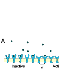
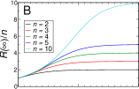
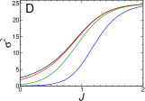
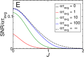
Figure 1: (A) Schematic diagram of cooperatively interacting receptors. Receptors interconvert between active and inactive states and preferentially bind ligand in the inactive state. The interaction energy $J$ between neighbors favors receptors in the same activity state. (B) The normalized static response $R(\infty)/n$ for closed chains (rings) of various lengths $n$ (for open chains, see sup ). (C) Response $R$, (D) noise $\sigma^{2}$, and (E) SNR as functions of coupling strength $J$ for a closed chain of $n=10$ receptors for various averaging times $\tau_{\text{avg}}$. In (E), the SNR is normalized by the averaging time.

The sensitivity to signal is quantified by the static response $R(\infty)=4\int_{0}^{\infty}\chi(t)dt$, which, when normalized by chain length, is the factor by which the DC (i.e. infinite time) response of a coupled receptor is amplified relative to that of an uncoupled receptor. The normalized static response $R(\infty)/n$ increases as a function of coupling strength from $1$ to $n$, as shown in Fig. 1B. At zero coupling, $J=0$, each receptor behaves independently and there is no cooperative amplification of the signal. As the coupling is increased, domains of adjacent receptors begin to effectively switch conformations together and the amplification $R(\infty)/n$ is determined by the size of these domains.

In practice, many cells have a limited measurement period and this can decrease the response $R(\tau_{\text{avg}})$, as shown in Fig. 1C. For a 1D ring, this dependence takes the simple form

$$R_{\textrm{ring}}(\tau_{\text{avg}})=R_{\textrm{ring}}(\infty)\left(1-\frac{\tau^{\textrm{ring}}_{c}}{\tau_{\text{avg}}}\left(1-e^{-\tau_{\text{avg}}/\tau^{\textrm{ring}}_{c}}\right)\right)$$ (7)

where

$$\tau^{\textrm{ring}}_{c}=1/(\alpha(1-\tanh(2J)))$$ (8)

is the response time, which increases exponentially with coupling strength due to the well-known phenomenon of critical slowing down Hohenberg and Halperin (1977). Notice that for any finite averaging time, the response eventually falls to zero with increasing coupling strength because the system slows down and cannot respond to the input in the time available. Intuitively, for large coupling $J$, the receptors become frozen in an all-active or all-inactive state, with switching between these states too slow to mediate a timely response to a changing input.

The intrinsic noise, i.e. the variance in time-averaged activity, increases monotonically with coupling strength, as shown in Fig. 1D. For the 1D ring,

$$\sigma_{\textrm{ring}}^{2}(\tau_{\text{avg}})=\sigma^{2}_{\textrm{ring}}(0)\mathcal{T}(\tau_{\text{avg}}/\tau^{\textrm{ring}}_{c}),$$ (9)

where $\tau_{c}$ is given in Eq. 8 and

$${\mathcal{T}}(x)=2(x+e^{-x}-1)/x^{2}.$$ (10)

For a given $J$, the maximal value of the noise occurs for zero averaging time (the “snapshot” limit), and is proportional to the static response as required by the fluctuation-dissipation theorem. Averaging for longer times substantially reduces the noise (via the factor $\mathcal{T}(\tau_{\text{avg}}/\tau^{\textrm{ring}}_{c})$), but time-averaging becomes less effective with increasing $J$ due again to critical slowing down, as the slower dynamics increases the correlation time $\tau_{c}$, the time required for fluctuations in activity to decay.

The relative uncertainty in sensing the concentration of ligand is determined by the signal-to-noise ratio (SNR), as shown in Fig. 1E, normalized per receptor,

$$\text{SNR}\equiv\frac{\text{SNR}_{\text{total}}}{N(\Delta f)^{2}}=\frac{(m\Delta A(\tau_{\text{avg}}))^{2}}{m\sigma^{2}(\tau_{\text{avg}})N(\Delta f)^{2}}=\frac{R^{2}(\tau_{\text{avg}})}{16n\sigma^{2}(\tau_{\text{avg}})}.$$ (11)

Surprisingly, the optimal value of the coupling strength $J$ to maximize the SNR is zero for all averaging times. That is, on a per receptor basis, independent receptors always have a lower total SNR than cooperative teams of receptors. For short averaging times, independent receptors have both a larger response and lower noise than teams. For longer averaging times, cooperative teams have a larger response, but independent receptors still achieve a higher SNR because their rapid switching leads to more independent samples of receptor activity and thus to a much lower time-averaged noise.

While the results in Fig. 1C-E are shown only for $n=10$, scaling analysis indicates that increasing the chain length $n$ will never make cooperative teams favorable with respect to uncoupled receptors. In the following, we derive how the SNR scales with the only two length scales in our model: the chain length $n$ and the correlation length $\xi$, which is the length scale over which the conformational states of neighboring receptors are correlated in an infinite system.

To best realize the cooperativity of a 1D chain of length $n$, the coupling strength has to be set to $J^{*}_{n}$, the smallest $J$ that gives approximately maximal response ($R(\infty)\approx n^{2}$), and the averaging time has to be just long enough for $R(\tau_{\text{avg}})$ to approach this maximum, i.e. $\tau_{\text{avg}}\approx\tau_{c}(J^{*}_{n})$. Longer times will reduce the noise, but by exactly the same factor for both the cooperative team and independent receptors, $\propto 1/\tau_{\text{avg}}$.

For the cooperative team, $\tau_{\text{avg}}=\tau_{c}(J_{n}^{*})$ is long enough that $R(\tau_{\text{avg}})\approx R(\infty)$, while $\sigma^{2}(\tau_{\text{avg}})\sim\sigma^{2}(0)$ (i.e. still roughly in the snapshot limit for noise). By the fluctuation-dissipation theorem, $\sigma^{2}(0)=R(\infty)/4$, so

$$\text{SNR}(J^{*}_{n})\approx\frac{R^{2}(\infty)}{16n\sigma^{2}(0)}=\frac{R(\infty)}{4n}\approx n/4\approx\xi(J^{*}_{n})/4.$$ (12)

Thus the SNR for the cooperative team is approximately equal to the chain length. The last approximate equality holds because the $J^{*}_{n}$ required for nearly maximal response yields an (infinite-chain) correlation length $\xi(J^{*}_{n})$ comparable to the actual chain length $n$.

By comparison, for $n$ independent receptors, the same averaging time $\tau_{\text{avg}}=\tau_{c}(J^{*}_{n})$ is long enough to reach the static response $R(\tau_{\text{avg}})\approx R(\infty)=n$, and for substantial noise reduction by time-averaging, $\sigma^{2}(\tau_{\text{avg}})\approx 2\sigma^{2}(0)/(\alpha\tau_{\text{avg}})$, so that

$$\text{SNR}(J=0) \approx \frac{R^{2}(\infty)}{32n\sigma^{2}(0)/(\alpha\tau_{\text{avg}})}=\frac{n^{2}}{8n^{2}/(\alpha\tau_{\text{avg}})}$$ (13)

$$= \frac{1}{8}\alpha\tau_{\text{avg}}\approx\frac{1}{8}\alpha\tau_{c}(J^{*}_{n}).$$

Therefore, for cooperative teams to be favorable with respect to uncoupled receptors requires $\xi(J^{*}_{n})>\frac{1}{2}\alpha\tau_{c}(J^{*}_{n})$, according to Eqs. 12 and 13. However, this will never happen for 1D chains because the correlation time grows faster than the correlation length with increasing $J$ in 1D, specifically $\tau_{c}\sim\xi^{2}$. In Fig. 2 we plot the ratio of SNRs for independent receptors versus cooperative receptors for closed chains.

Figure 2: Ratio of the SNR for independent receptors to the SNR for cooperative receptors as a function of the correlation length $\xi$ for a 1D ring and a 2D square lattice of $n=100$ receptors with periodic boundary conditions, as well as mean field theory (MFT). Averaging times are $\alpha\tau_{\text{avg}}=100$ (solid curve) and $\alpha\tau_{\text{avg}}=\infty$ (dashed curve), with power law plots for comparison (dotted lines).

The ratio never favors cooperative receptors and, in the long-averaging-time limit, follows the expected scaling $\sim\xi$ for $\xi\ll n$ and $\sim\xi^{2}$ for $\xi\gg n$. A shorter averaging time only makes things worse for cooperative receptors, as in this case the expected scaling is still $\sim\xi$ for $\xi\ll n$, but $\sim\xi^{4}$ for $\xi\gg n$ sup .

Our results naturally generalize to higher-dimensional coupling. For 2D, the most natural topology for interacting membrane receptors, the ratio of uncoupled to coupled SNRs for long averaging times $\tau_{\text{avg}}\gg\tau_{c}$ scales as $\text{SNR}(J=0)/\text{SNR}(J)\rightarrow n\alpha\tau_{c}/R(\infty)\sim\xi^{z-\gamma/\nu}\approx\xi^{0.41}$ sup  , as seen in Fig. 2 in the expected regime $\xi\ll\sqrt{n}$. As in 1D, independent receptors do better than coupled receptors, but this advantage grows more slowly with correlation length in 2D.

High dimensional ($D\geq 4$), or global coupling of receptors, which could be mediated by the cell membrane or by rapidly diffusing effectors, is described by the mean field limit of the Ising model. In this limit, the dynamics of cluster activity reduces to that of an overdamped harmonic oscillator, and the normalized static response and correlation time are both equal, $R^{\text{MFT}}(\infty)/n=\alpha\tau_{c}^{\text{MFT}}=1/(1-\zeta J)$, where $\zeta$ is the number of nearest neighbors. Consequently, for long averaging times, the ratio of SNRs for independent versus coupled receptors is constant. Thus, at best, increasing the dimension of receptor coupling yields parity between cooperative and independent receptors.

More generally, the universal behavior of Ising models near the phase transition and a rigorous bound on Ising critical exponents $\nu z\geq\gamma$ Abe and Hatano (1969) suggest that critical slowing down is unavoidable and independent receptors will always optimize the SNR. We have also studied the addition of other potential noise sources, including slow ligand dynamics and static variation of receptor offset energies, and find that independent receptors still yield the best SNR sup .

In summary, we developed a physical description of cooperativity based on the principle that allosteric interactions between receptor proteins are inherently local. From our simple Ising-type model, which encompasses a broad class of models, we elucidated the relationship between cooperativity and intrinsic noise. We found that the slowing down of receptor switching due to cooperative interactions strongly impairs the SNR and that consequently the SNR is always highest for zero receptor cooperativity, even though the absolute sensitivity is optimized for nonzero cooperativity. Since our SNR is normalized by receptor number and stimulus strength, our results show that (i) for a given small stimulus, independent receptors achieve SNR $>1$ for the fewest receptors, and (ii) for a given number of receptors, independent receptors achieve SNR $>1$ for the smallest stimulus strength.

Our surprising result offers a fresh perspective on bacterial chemotaxis, by indicating that the network is not simply optimizing SNR, since the observed receptor cooperativity in this system reduces the SNR by a factor of $\sim 50$ . More generally, our result reveals that the benefits of cooperativity for sensing are far from obvious, potentially explaining the absence of receptor cooperativity in many sensory networks.