A Weakened Cascade Model for Turbulence in Astrophysical Plasmas

Abstract

A refined cascade model for kinetic turbulence in weakly collisional astrophysical plasmas is presented that includes both the transition between weak and strong turbulence and the effect of nonlocal interactions on the nonlinear transfer of energy. The model describes the transition between weak and strong MHD turbulence and the complementary transition from strong kinetic Alfvén wave (KAW) turbulence to weak dissipating KAW turbulence, a new regime of weak turbulence in which the effects of shearing by large scale motions and kinetic dissipation play an important role. The inclusion of the effect of nonlocal motions on the nonlinear energy cascade rate in the dissipation range, specifically the shearing by large-scale motions, is proposed to explain the nearly power-law energy spectra observed in the dissipation range of both kinetic numerical simulations and solar wind observations.

I Introduction

Plasma turbulence plays an important role in the transfer of energy in a wide range of space and astrophysical environments, from clusters of galaxies, to accretion disks around black holes, to the magnetized corona of our own sun, to the solar wind that fills the heliosphere. In all of these diverse environments, turbulence is responsible for the transport of energy from the large scales at which the turbulence is driven down to the small scales at which dissipation mechanisms can effectively dissipate the turbulent fluctuations and lead to heating of the plasma species. The understanding of plasma turbulence, its dissipation, and the resulting plasma heating is therefore a key goal for the space physics and astrophysics communities.

Although the study of the inertial range of plasma turbulence—the range of scales over which the effects of driving and dissipation are negligible—dates back more than four decades Coleman:1968 , study of the dissipation range has only recently become a focus of the astrophysics and heliospheric physics communities. One of the major challenges in the investigation of the dissipation mechanisms at work in space and astrophysical plasmas is the fact that, at the small scales on which these mechanisms operate, the dynamics is typically weakly collisional. Under these conditions, a kinetic description of the plasma dynamics is necessary Marsch:1991 ; Marsch:2006 ; Howes:2008c ; Howes:2008b ; Howes:2008d ; Schekochihin:2009 , a much more complicated description than the standard fluid descriptions, such as magnetohydrodynamics (MHD), commonly used in the study of the inertial range dynamics.

The increasingly vigorous activity studying the dissipation of plasma turbulence has been driven by several new developments: the development of new analytical models of kinetic turbulence Howes:2008c ; Howes:2008b ; Schekochihin:2009 , advances in high-performance computation that have made possible kinetic simulations of weakly collisional turbulence Howes:2008a ; Howes:2011a , and, most recently, new observational studies of turbulence in the solar wind with sufficient time resolution to extend the satellite-frame frequency power spectra of magnetic and electric field fluctuations up to the Doppler-shifted frequencies associated with the electron Larmor radius Sahraoui:2009 ; Kiyani:2009 ; Alexandrova:2009 ; Chen:2010 ; Sahraoui:2010b .

This paper presents the refinement of a turbulent cascade model for weakly collisional plasmas, originally devised by Howes et al. 2008 Howes:2008b . At the small scales where the turbulent motions are dissipated, two new physical effects may play a significant role: the transition between weak and strong turbulence, and the nonlocal contribution to the nonlinear energy transfer rate. The aim of this paper is to describe how these additional physical effects are incorporated into a refined model, denoted the weakened cascade model. Energy spectra predicted by the new model are compared in detail to the numerical energy spectra from nonlinear gyrokinetic simulations of turbulence in the dissipation range, and the physical implications of the nonlocal contribution to the nonlinear energy transfer in the dissipation range are discussed in detail.

II Motivation for a Refined Cascade Model

A new and exciting challenge in the study of turbulence in the solar wind is to understand the recent observations of nearly power-law magnetic energy spectra in the dissipation range Note0 up to scales corresponding to the electron Larmor radius Sahraoui:2009 ; Kiyani:2009 ; Alexandrova:2009 ; Chen:2010 ; Sahraoui:2010b . The physics describing the turbulent dynamics of the inertial range is expected to be self-similar, dominated by the conditions that are “local” in scale Kolmogorov:1941 . In the dissipation range, on the other hand, dissipative mechanisms necessarily play a non-negligible role, and so the usual assumption that the turbulent energy transfer is dominated by local interactions must be called into question.

In anisotropic Alfvénic turbulence, nonlinear interactions typically strengthen as the cascade progresses to smaller scale until they reach and maintain a state of critically balanced, strong turbulence. But as turbulent fluctuation amplitudes are diminished by some physical dissipation mechanism, one must consider the possibility that the turbulence may eventually transition back to a state of weak turbulence. In addition to this transition from strong to weak turbulence, one must also account for the effect on the nonlinear energy transfer rate at small scales (where the local turbulent fluctuation amplitudes are diminished by some dissipation mechanism) by the undamped, nonlocal turbulent motions at larger scales. In this section, we briefly review the relevant concepts from modern theories of anisotropic magnetized turbulence that provide the theoretical foundation for these arguments. Then we identify the shortcomings of the original cascade model Howes:2008b and outline the necessary refinements of the model to account for the transition to weak turbulence at dissipative scales and for the effect of nonlocal motions on the energy cascade rate.

II.1 Review of Anisotropic Plasma Turbulence Theories

Early theories of magnetized plasma turbulence proposed an isotropic cascade of turbulent energy from low wavenumbers (large scales) to large wavenumbers (small scales) Iroshnikov:1963 ; Kraichnan:1965 . Measurements of magnetized plasma turbulence both in the laboratory Robinson:1971 ; Zweben:1979 ; Montgomery:1981 and in the solar wind Belcher:1971 , as well as early numerical simulations Shebalin:1983 , demonstrated the existence of significant anisotropy with respect to the direction of the local mean magnetic field. In the context of incompressible MHD, the inclusion of anisotropy in the direction of the nonlinear turbulent energy transfer through wavevector space lead to a fundamental distinction between the properties of weak MHD turbulence and strong MHD turbulence Sridhar:1994 ; Goldreich:1995 . As the shift in behavior between strong and weak turbulence plays a role when the turbulent cascade suffers dissipation, a brief review of the relevant properties is provided here.

Although the theory for weak turbulence in incompressible MHD plasmas was a focal point of controversy in the late 1990s Sridhar:1994 ; Montgomery:1995 ; Ng:1996 ; Goldreich:1997 ; Ng:1997 ; Galtier:2000 ; Lithwick:2003 , a refined theory of weak MHD turbulence has emerged. This theory is based on a perturbative treatment of weak, resonant three-wave interactions between Alfvén waves propagating in opposite directions along the local mean magnetic field. The need to satisfy both the resonance conditions for frequency and wavevector Shebalin:1983 and the requirement that only counter-propagating Alfvén waves interact nonlinearly Iroshnikov:1963 ; Kraichnan:1965 leads to the prediction that there is no parallel cascade of energy in wavenumber space (where the directions parallel and perpendicular are defined with respect to the local mean magnetic field). Therefore, energy is transferred via the turbulent cascade anisotropically in wavevector space, only to higher perpendicular wavenumbers $k_{\perp}$, while the characteristic parallel wavenumber $k_{\parallel}$ remains constant. The one-dimensional magnetic energy spectrum $E_{B}(k_{\perp})$, defined such that the total magnetic energy $E_{B}=\int dk_{\perp}E_{B}(k_{\perp})$, is predicted to scale as $E_{B}(k_{\perp})\propto k_{\perp}^{-2}$. Recent reduced MHD numerical simulations have confirmed this predicted scaling in the regime of weak turbulence Perez:2008 . The nonlinear interactions strengthen as the perpendicular wavenumber increases, so as the turbulent cascade progresses to higher $k_{\perp}$, the dynamics eventually violate the assumption of weak nonlinear interactions required for the application of perturbation theory. Therefore, the theory of weak MHD turbulence predicts that, if a sufficiently large inertial range exists, weak MHD turbulence will eventually transition to a state of strong MHD turbulence Sridhar:1994 ; Goldreich:1995 .

When the turbulence becomes sufficiently strong, the perturbative expansion of the nonlinear term is no longer dominated by the three-wave interactions, and terms of all orders contribute. This leads to a broadening of the resonance, relaxing the strict constraints on the frequency and wavevector, making possible the cascade of energy in the parallel direction of wavevector space Goldreich:1995 . The theory of strong turbulence in incompressible MHD plasmas is based on the conjecture of a critical balance Higdon:1984a ; Goldreich:1995 between the linear timescale for Alfvén waves and the nonlinear timescale of turbulent energy transfer. The one-dimensional magnetic energy spectrum is predicted to scale as $E_{B}(k_{\perp})\propto k_{\perp}^{-5/3}$. The conjecture of critical balance predicts the development of a scale-dependent anisotropy given by $k_{\parallel}\propto k_{\perp}^{2/3}$; therefore, the one-dimensional parallel magnetic energy spectrum, defined by $E_{B}=\int dk_{\parallel}E_{B}(k_{\parallel})$, is predicted to scale as $E_{B}(k_{\parallel})\propto k_{\parallel}^{-2}$. The predictions of the scale-dependent anisotropy are supported by early numerical simulations Cho:2000 ; Maron:2001 and by more recent studies of the scaling of the the parallel spectrum in the solar wind Horbury:2008 ; Podesta:2009a .

The lack of a parallel cascade in weak MHD turbulence and the scale dependent anisotropy in strong MHD turbulence have an important consequence: even when turbulence is driven isotropically at low wavenumber (large scale) with $k_{0}=k_{\perp 0}=k_{\parallel 0}$, for a sufficiently large inertial range (typical of most space and astrophysical plasmas of interest), the turbulent fluctuations at high wavenumber (small scale) become significantly anisotropic with $k_{\parallel}\ll k_{\perp}$. When the turbulent cascade reaches the perpendicular scale of the ion Larmor radius $k_{\perp}\rho_{i}\sim 1$, such turbulent fluctuations transition to a cascade of strong kinetic Alfvén wave (KAW) turbulence, as has been predicted theoretically Gruzinov:1998 ; Quataert:1999 ; Howes:2008b ; Schekochihin:2009 and verified with nonlinear kinetic simulations Howes:2008a . Assuming again a critical balance between the linear and nonlinear timescales, in the absence of dissipation, the kinetic Alfvén wave cascade is predicted to have a one-dimensional magnetic energy spectrum that scales as $E_{B}(k_{\perp})\propto k_{\perp}^{-7/3}$ and a scale-dependent anisotropy $k_{\parallel}\propto k_{\perp}^{1/3}$ for the nonlinear transfer of energy in wavevector space Biskamp:1999 ; Cho:2004 ; Krishan:2004 ; Dastgeer:2005 ; Howes:2008b ; Schekochihin:2009 . When collisionless dissipation via the Landau resonance is included, the original cascade model Howes:2008b predicts that, if magnetometer noise floor is taken into account, the spectral index of the measured one-dimensional magnetic energy spectrum could vary from a value of $-7/3$ for weak dissipation up to approximately $-4$ for strong dissipation, with the strength of the dissipation depending on the plasma parameters $\beta_{i}$ and $T_{i}/T_{e}$.

Figure 1: Schematic diagram of the anisotropic transfer of energy through wavevector space $(k_{\perp},k_{\parallel})$. For turbulence driven isotropically at low wavenumber $k_{\perp 0}\rho_{i}\sim k_{\parallel 0}\rho_{i}\sim 10^{-6}$ (quarter circle in the lower left of the figure), nonlinear interactions lead to transfer of energy to higher wavenumbers. For weak MHD turbulence, the transfer is restricted to higher $k_{\perp}$, with no cascade of energy to higher parallel wavenumbers $k_{\parallel}$. As the MHD turbulence becomes strong (at $k_{\perp}\rho_{i}\sim 10^{-3}$), resonance broadening allows a parallel cascade of energy that achieves a state of critical balance at all scales, with $k_{\parallel}\propto k_{\perp}^{2/3}$. Finally, as the strong MHD turbulence transitions to strong KAW turbulence (at $k_{\perp}\rho_{i}\sim 1$), the turbulence remains in critical balance but the scaling in this regime changes to $k_{\parallel}\propto k_{\perp}^{1/3}$.

To highlight the different behaviors predicted for weak MHD, strong MHD, and strong KAW turbulence, a schematic of the energy transfer through wavevector space is presented in Figure 1. Since the dynamics of an MHD plasma is axisymmetric about the direction of the local mean magnetic field, the description of energy transfer through the three-dimensional wavevector space can be reduced to the two-dimensional plane of the parallel component of the wavevector $k_{\parallel}$ (the axial coordinate parallel to the local mean magnetic field) and the perpendicular component $k_{\perp}$ (the radial coordinate perpendicular to the local mean magnetic field). The anisotropic MHD turbulence theories above suggest that the energy flows through wavenumber space along the path given by the solid line in Figure 1—along constant $k_{\parallel}$ for weak MHD turbulence and along a path given by critical balance for strong MHD and strong KAW turbulence. Numerical simulations of MHD turbulence Cho:2000 ; Maron:2001 ; Cho:2002 ; Cho:2003 ; Oughton:2004 , however, suggest that the turbulent energy does not flow strictly along this one-dimensional path through wavevector space but approximately fills the shaded region in Figure 1. Similar to the original cascade model, the one-dimensional weakened cascade model presented in this paper determines the turbulent energy integrated vertically in this figure over all possible values of $k_{\parallel}$ at each $k_{\perp}$; the effective value of $k_{\parallel}$ for the integrated turbulent energy at each $k_{\perp}$ is assumed to be given by the solid line in Figure 1.

Several final comments regarding plasma turbulence theories are in order. First, note that the plot of the $(k_{\perp},k_{\parallel})$ plane in Figure 1 is logarithmic on both axes. The inherently anisotropic transfer of energy in magnetized plasma turbulence naturally leads to a condition in which $k_{\parallel}\ll k_{\perp}$ at high wavenumbers. A number of studies of solar wind turbulence in the past have assumed a constant angle between the direction of the wavevector and the local mean magnetic field, which would correspond to a line with $k_{\parallel}\propto k_{\perp}$ on the logarithmic plot of wavevector space; this leads to a significant underestimate of the anisotropy at small scales (multi-spacecraft measurements in the solar wind demonstrate significant anisotropy at the scale of the ion Larmor radius Sahraoui:2010b ). Second, although much of the weak and strong MHD turbulence theory applies rigorously only to incompressible MHD plasmas, it is our view that the fundamental concepts derived for incompressible MHD plasmas offer useful guidance for the understanding of turbulence in plasmas allowing a wider range of physical effects, e.g., compressibility, finite Larmor radius effects, linear kinetic damping. Finally, although we choose the particular strong turbulence scaling given by Goldreich and Sridhar Goldreich:1995 as the basis for the original and weakened cascade models, an alternative theory for the scaling of strong MHD turbulence has been proposed by Boldyrev Boldyrev:2006 ; application of the weakened cascade model using the Boldyrev scaling will be discussed in a subsequent paper.

II.2 The Original Cascade Model

The aim of the original cascade model Howes:2008b is to explain the observed magnetic energy spectrum in the solar wind using a minimal number of ingredients, namely, finite Larmor radius effects and kinetic damping via the Landau resonance. This model employs a one-dimensional continuity equation for the magnetic energy spectrum in perpendicular wavenumber space, and is based on three assumptions: (a) the Kolmogorov hypothesis that the energy transfer is determined locally in wavenumber spaceKolmogorov:1941 ; (b) that a state of critical balance exists between the linear and nonlinear timescales at all wavenumbers in the spectrum Higdon:1984a ; Goldreich:1995 ; and (c) that the linear kinetic damping rates determine the dissipation of the turbulent fluctuations even in the presence of the nonlinear cascade. Results of the model generally demonstrate the qualitative feature that, as the linear kinetic damping becomes strong, the spectrum begins an exponential fall off. This qualitative feature is observed neither in recent nonlinear kinetic simulations Howes:2011a nor in recent observations of the dissipation range of the solar wind Sahraoui:2009 ; Kiyani:2009 ; Alexandrova:2009 ; Chen:2010 ; Sahraoui:2010b .

The failure of the original cascade model to reproduce the correct qualitative behavior when collisionless damping becomes strong is due to the assumption of strong turbulence satisfying the critical balance condition at all scales. It seems relatively clear that, as collisionless damping reduces the turbulent amplitude at a given wavenumber to a level below that expected for a dissipationless cascade, the nonlinear turbulent interactions at that wavenumber must cease to be strong. One then expects a transition to a cascade with weak nonlinear interactions (in the sense of weak turbulence), although the collisionless damping and shearing by larger scale motions will also play an important role, so it won’t be a standard weak turbulence picture.

The failure of the strong turbulence assumption at perpendicular wavenumbers where the dissipation becomes significant is made clear by a simple physical argument applied to the original cascade model results. In Figure 7 of the original cascade model paper Howes:2008b , the parallel wavenumber as a function of the perpendicular wavenumber, $k_{\parallel}(k_{\perp})$, is plotted for plasma parameters $\beta_{i}=1$ and $T_{i}/T_{e}=1$. At a value of $k_{\perp}\rho_{i}\simeq 8$, the value of $k_{\parallel}$ peaks, and then it begins to drop. Physically, this would mean that, as the turbulence continues to cascade to smaller perpendicular scales, its parallel scale length actually increases. This predicted behavior does not make physical sense. This point is discussed at length in paragraph [46] of that paper, with the forward looking conclusion that “nonlinear simulations are necessary to determine accurately the behavior of the turbulent cascade as the kinetic damping becomes significant.”

II.3 Weak Turbulence and Nonlocal Interactions

The more likely physical result, when the turbulence is dissipatively weakened, is that the cascade to higher parallel wavenumber is suppressed, so the parallel wavenumber remains constant. Weak turbulence theory predicts that the parallel cascade is suppressed in incompressible MHD plasmas Galtier:2000 , but whether this also holds in the kinetic Alfvén wave regime is not known. We conjecture here that the parallel cascade is suppressed for weak kinetic Alfvén wave turbulence, as discussed in more detail in §III.1. In addition to this effect, the nonlinear transfer of energy in weak turbulence also requires many uncorrelated “collisions” between counter-propagating Alfvén wave packets, in contrast to the single collision required in strong turbulence Sridhar:1994 ; Goldreich:1995 .

Therefore, the weakened cascade model proposed here describes the transition between strong and weak turbulence by incorporating two changes: (1) altering the cascade in parallel wavenumber; and (2) increasing the number of Alfvén wave collisions required to accomplish nonlinear energy transfer. The consequence of these changes, however, is that the collisionless damping at a given scale becomes relatively stronger than the nonlinear transfer, causing the spectra to cut-off even more abruptly, resulting in even greater discrepancy between the cascade model predictions and both the numerical simulations and the solar wind observations.

To resolve this discrepancy requires the incorporation of another physical effect, in addition to the transition to weak turbulence. It requires accounting for the effect on the nonlinear energy transfer rate at a given scale by turbulent motions at other scales. Consider specifically the nonlinear turbulent energy transfer at a particular perpendicular wavenumber $k_{\perp*}$. Although the turbulent energy is still transferred locally in scale space—for example, energy transfer from wavenumber $k_{\perp*}$ to $2k_{\perp*}$— this nonlinear energy transfer is not only due to motions at the local wavenumber $k_{\perp*}$, but also due to nonlocal (in scale space) motions at smaller and larger wavenumbers. Both coherent shearing by motions at low wavenumbers $k_{\perp}<k_{\perp*}$ (large scales) and incoherent diffusion by motions at high wavenumbers $k_{\perp}>k_{\perp*}$(small scales) may contribute substantially to the total nonlinear energy transfer rate from $k_{\perp*}$ to $2k_{\perp*}$. Therefore, we must abandon the Kolmogorov hypothesis of locality and account for the effect of nonlocal interactions on the turbulent energy transfer.

The physical effect due to shearing by large scale motions is essentially the same as that seen in high magnetic Prandtl number dynamo simulations using MHD Schekochihin:2004d . The magnetic Prandtl number is defined by the ratio of viscosity over the magnetic diffusivity, $\mbox{Pr}_{m}=\nu/\eta$, and typically $\mbox{Pr}_{m}\gg 1$ for many astrophysical plasmas of interest. For a high magnetic Prandtl number plasma, magnetic energy can be supported on subviscous scales, and this magnetic energy is observed in simulations to cascade to ever smaller scales, until the resistive scale is reached, at which point the magnetic energy can be dissipated. This cascade occurs although the plasma cannot support any fluid motions at the subviscous scales of interest. The transfer of magnetic energy at these small, subviscous scales is accomplished by the shearing due to larger scale motions (at scales larger than the viscous cut-off). This energy transfer is therefore nonlocal in nature.

Such an effect must come into play in a weakly collisional plasma when the turbulent cascade reaches a small enough perpendicular scale that collisionless damping can diminish the amplitude of the local (in scale) turbulent fluctuations. Kolmogorov’s locality assumption is well supported in the inertial range, because the energy cascade rate due to shearing by local fluctuations always dominates over the energy cascade rate due to shearing by larger-scale motions. But, in the dissipation range, where the local fluctuations begin to diminish in amplitude due to some dissipative mechanism, their dominance of the local energy cascade rate breaks down, and the effects of shearing by larger-scale, undamped motions must be taken into account. In this way, the energy cascade rate at the small, rather strongly damped scales may be dominated by this nonlocal shearing, with the weak turbulent interactions due to local fluctuations playing a subdominant role. Thus, the energy can be cascaded to ever smaller scale at a reasonably large rate even though the nonlinear energy transfer rate due to the local fluctuations becomes negligible. This nonlocal shearing effect is proposed to explain the nearly power-law appearance of the numerical and observational spectra, and is critical for understanding the turbulence in the dissipation range. The nonlocal contribution to the energy cascade rate by diffusive motions at small scales, although negligible at the far end of the dissipation range, is also included in the refined model for consistency.

III The Weakened Cascade Model

In order to refine the original cascade model Howes:2008b , we must incorporate two physical effects not included in the original model:

1. Weak Turbulence: The model must be able to handle the quantitative changes in the energy cascade rate in both the weak and strong turbulence regimes. Of particular importance is the qualitative difference in the parallel cascade of energy: in weak turbulence, there is no cascade of energy to smaller parallel scales; and in strong turbulence, the parallel cascade is governed by critical balance.

2. Nonlocal Interactions: The net energy cascade rate at a given wavenumber $\epsilon(k_{\perp*})$ must account for the nonlinear transfer due to both the local fluctuations at $k_{\perp*}$ and nonlocal fluctuations at other wavenumbers. The nonlocal fluctuations contribute to the nonlinear energy cascade rate due to shearing by fluctuations at smaller wavenumbers $k_{\perp}<k_{\perp*}$ and diffusion by fluctuations at larger wavenumbers $k_{\perp}>k_{\perp*}$.

In this section, we describe in detail the quantitative modifications of the original cascade model required to incorporate these two physical effects, resulting in the new weakened cascade model.

III.1 Weak Turbulence

The key parameter in distinguishing weak from strong turbulence is the nonlinearity parameter

$$\chi\sim\frac{k_{\perp}v_{\perp}}{\omega}.$$ (1)

This dimensionless parameter $\chi$ measures the ratio of the nonlinear frequency $\omega_{nl}\simeq k_{\perp}v_{\perp}$ to the linear wave frequency $\omega$. Strong turbulence corresponds to $\chi\sim 1$, satisfying the condition of critical balance $\omega\sim\omega_{nl}$, whereas weak turbulence corresponds to $\chi\ll 1$. Note that the case of overdriven turbulence $\chi>1$ has not been thoroughly explored or discussed in the literature; it probably deserves some attention, but henceforth we will consider only the cases of weak or critically balanced turbulence $\chi\lesssim 1$.

To handle the transition to kinetic Alfvén wave turbulence, we focus on the magnetic energy rather than the kinetic energy, so we want to write the nonlinear energy cascade rate in terms of the magnetic fluctuation energy, $b_{k}^{2}\equiv\delta B^{2}_{\perp}(k_{\perp})/4\pi n_{i}m_{i}$, where we have written the magnetic field fluctuation in velocity units. We also adopt the shorthand $v_{k}\equiv v_{\perp}(k_{\perp})$. Following the original cascade model, we relate the velocity and magnetic field fluctuations to each other using the linear theory,

$$v_{k}=\pm\alpha(k_{\perp})b_{k},$$ (2)

where the coefficient $\alpha$ smoothly transitions from the MHD to the KAW limit,

$$\alpha(k_{\perp})=\left\{\begin{array}[]{cc}1,&k_{\perp}\rho_{i}\ll 1\\ k_{\perp}\rho_{i}/{\sqrt{\beta_{i}+2/(1+T_{e}/T_{i})}},&k_{\perp}\rho_{i}\gg 1\end{array}\right.$$ (3)

Note that the linear frequency in the gyrokinetic limit Note1 is given by

$$\omega=\pm\overline{\omega}(k_{\perp})k_{\parallel}v_{A}.$$ (4)

where $\overline{\omega}(k_{\perp})=\alpha(k_{\perp})$ in both asymptotic ranges $k_{\perp}\rho_{i}\ll 1$ and $k_{\perp}\rho_{i}\gg 1$ but not in the transition region $k_{\perp}\rho_{i}\sim 1$. For this simple model, we take the approximation that $\alpha(k_{\perp})=\overline{\omega}(k_{\perp})$ over all scales.

Thus, an appropriate definition of the nonlinearity parameter valid for all scales is

$$\chi=\frac{C_{2}k_{\perp}v_{k}}{\omega}=\frac{C_{2}k_{\perp}b_{k}\alpha}{k_{\parallel}v_{A}\alpha}=\frac{C_{2}k_{\perp}b_{k}}{k_{\parallel}v_{A}},$$ (5)

where $C_{2}$ is an order-unity, dimensionless “Kolmogorov” constant.

There are two primary effects that must be captured in order to incorporate the weak turbulence limit into the cascade model:

1. Slower nonlinear energy cascade rate due to the effect of many uncorrelated weak interactions between oppositely directed Alfvén waves Sridhar:1994 .

2. The suppression of the energy cascade to small parallel scales.

These issues are addressed separately below.

We define the energy cascade rate by

$$\epsilon(k_{\perp})=C_{1}^{-3/2}\omega_{nl}b_{k}^{2}.$$ (6)

where $C_{1}$ is an order-unity, dimensionless Kolmogorov constant and the nonlinear frequency, bridging weak and strong turbulence, is given by

$$\omega_{nl}=\chi k_{\perp}v_{k}=\left(\frac{C_{2}k_{\perp}b_{k}}{k_{\parallel}v_{A}}\right)k_{\perp}b_{k}\alpha.$$ (7)

Note that the cascade time is given by

$$\tau_{nl} = \omega_{nl}^{-1}=\left(\frac{k_{\parallel}v_{A}}{C_{2}k_{\perp}b_{k}}\right)(k_{\perp}b_{k}\alpha)^{-1}$$ (8)

$$= \left(\frac{k_{\parallel}v_{A}}{C_{2}k_{\perp}b_{k}}\right)^{2}C_{2}(k_{\parallel}v_{A}\alpha)^{-1}=N^{2}C_{2}(k_{\parallel}v_{A}\alpha)^{-1}.$$ (9)

This shows explicitly that, in the MHD limit $\alpha=1$, it takes $N^{2}=1/\chi^{2}$ Alfven wave packet collisions, each lasting an Alfvén wave crossing time $\tau_{A}=(k_{\parallel}v_{A})^{-1}$, for the energy at a given scale to be transferred to the next scale.

In summary, the energy cascade rate may be written

$$\epsilon(k_{\perp})=C_{1}^{-3/2}\left(\frac{C_{2}k_{\perp}b_{k}}{k_{\parallel}v_{A}}\right)k_{\perp}b_{k}^{3}\alpha.$$ (10)

Let us investigate the predicted steady-state magnetic energy spectrum in different limits for a constant energy cascade rate $\epsilon$.

In the MHD limit, $\alpha=1$. The critically balanced, strong turbulence limit gives $\chi=C_{2}k_{\perp}b_{k}/k_{\parallel}v_{A}=1$, so we have $\epsilon=C_{1}^{-3/2}k_{\perp}b_{k}^{3}$, yielding a solution for the magnetic field $b_{k}=C_{1}^{1/2}\epsilon^{1/3}k_{\perp}^{-1/3}$ and a corresponding 1-D magnetic energy spectrum $E_{B}(k_{\perp})=b_{k}^{2}/k_{\perp}=C_{1}\epsilon^{2/3}k_{\perp}^{-5/3}$. In the weak turbulence limit $\chi<1$, we have $\epsilon=C_{1}^{-3/2}C_{2}k_{\perp}^{2}b_{k}^{4}/k_{\parallel}v_{A}$ and $k_{\parallel}$ remains constant, so we obtain a solution for the magnetic field $b_{k}=C_{1}^{3/8}C_{2}^{-1/4}\epsilon^{1/4}(k_{\parallel}v_{A})^{1/4}k_{\perp}^{-1/2}$ and a corresponding 1-D magnetic energy spectrum $E_{B}(k_{\perp})=C_{1}^{3/4}C_{2}^{-1/2}\epsilon^{1/2}(k_{\parallel}v_{A})^{1/2}k_{\perp}^{-2}$.

In the KAW limit, we approximate $\alpha\simeq k_{\perp}\rho_{i}$. Strong, critically balanced KAW turbulence also has $\chi=C_{2}k_{\perp}b_{k}/k_{\parallel}v_{A}=1$, so we have $\epsilon=C_{1}^{-3/2}k_{\perp}^{2}\rho_{i}b_{k}^{3}$, yielding a solution for the magnetic field $b_{k}=C_{1}^{1/2}\epsilon^{1/3}k_{\perp}^{-2/3}\rho_{i}^{-1/3}$ and a corresponding 1-D magnetic energy spectrum $E_{B}(k_{\perp})=C_{1}\epsilon^{2/3}k_{\perp}^{-7/3}\rho_{i}^{-2/3}$. In the weak turbulence limit $\chi<1$, we have $\epsilon=C_{1}^{-3/2}C_{2}k_{\perp}^{3}b_{k}^{4}\rho_{i}/k_{\parallel}v_{A}$. In this case, we assume that $k_{\parallel}$ remains constant in the weak turbulence limit; this assumption is discussed later in this subsection. The solution for the magnetic field is then $b_{k}=C_{1}^{3/8}C_{2}^{-1/4}\epsilon^{1/4}(k_{\parallel}v_{A})^{1/4}k_{\perp}^{-3/4}\rho_{i}^{-1/4}$ and a corresponding 1-D magnetic energy spectrum $E_{B}(k_{\perp})=C_{1}^{3/4}C_{2}^{-1/2}\epsilon^{1/2}(k_{\parallel}v_{A})^{1/2}k_{\perp}^{-5/2}\rho_{i}^{-1/2}$, agreeing with theoretical predictions for weak KAW turbulence Galtier:2006 .

The other important effect when synthesizing a theory that combines the weak and strong turbulence limits and their influence on the turbulent cascade of energy is to model the parallel cascade of energy. In the strong limit, the condition of critical balance allows the determination of $k_{\parallel}(k_{\perp})$, strictly a function of $k_{\perp}$. The assumption of critical balance at all scales in the original cascade model allowed the damping term to be simplified. The original cascade model equation for the evolution of the magnetic energy was written as

$$\frac{\partial b_{k}^{2}}{\partial t}=-k_{\perp}\frac{\partial\epsilon(k_{\perp})}{\partial k_{\perp}}+S(k_{\perp})-2{\gamma}b_{k}^{2},$$ (11)

where the last term could be simplified, under the assumption of critical balance and for the linear kinetic damping rate in the gyrokinetic limit $\gamma=\pm\overline{\gamma}(k_{\perp})k_{\parallel}v_{A}$, to take the form

$$-2C_{1}^{3/2}C_{2}\frac{\overline{\gamma}(k_{\perp})}{\overline{\omega}(k_{\perp})}\epsilon(k_{\perp}),$$ (12)

strictly a function of $k_{\perp}$. When this assumption is relaxed, however, to determine the damping rate one needs to know the value of $k_{\parallel}(k_{\perp})$ to find

$$\gamma(k_{\perp},k_{\parallel})=\overline{\gamma}(k_{\perp})k_{\parallel}v_{A}.$$ (13)

Without critical balance, we must devise some other means of determining an appropriate value of $k_{\parallel}$.

It must be noted that the distribution of turbulent power in the plasma can fill a region of the two-dimensional wave vector space $(k_{\perp},k_{\parallel})$, as denoted by the shaded region in Figure 1. Here we follow the original cascade model in treating the magnetic fluctuation energy integrated over all possible values of $k_{\parallel}$, so that

$$b_{k}^{2}(k_{\perp})=\int dk_{\parallel}\delta B^{2}_{\perp}(k_{\perp},k_{\parallel})/4\pi n_{i}m_{i}.$$ (14)

We will treat the total magnetic energy as if it resides at a single value of $k_{\parallel}$. The particular choice we make is the maximum value of $k_{\parallel}$ that contains significant fluctuation energy. Therefore, in the strong turbulence limit, $k_{\parallel}$ is chosen so that the parallel cascade satisfies the critical balance criterion. In the weak turbulence limit, however, we assume that the parallel cascade of energy is inhibited, so the value of $k_{\parallel}$ remains constant as energy cascades to larger $k_{\perp}$. By making this choice, we again can solve for the turbulent cascade of magnetic energy as a one-dimensional problem in $k_{\perp}$, but as we shall see this necessitates solving for $k_{\parallel}$ from the driving wavenumber on up.

It has been proven rigorously that there is no parallel cascade of energy for weak turbulence in the limit of incompressible MHD Galtier:2000 . Heuristic arguments for weak turbulence in incompressible Hall MHD plasmas Galtier:2006 and numerical evidence demonstrating an anisotropic cascade of energy in weak whistler wave turbulence Gary:2008 ; Saito:2008 ; Gary:2010 suggest that the parallel cascade is also suppressed for the dispersive wave modes at perpendicular scales smaller than the ion Larmor radius. Therefore, we conjecture that the parallel cascade is suppressed in weak kinetic Alfvén wave turbulence as well Note6 . Nonlinear kinetic simulations of turbulence in the kinetic Alfvén wave regime will play a key role in testing this hypothesis.

To model these effects, we take the equation for the evolution of the parallel wavenumber to be

$$\frac{d\ln k_{\parallel}}{d\ln k_{\perp}}=\left[\frac{2/3+(1/3)(k_{\perp}\rho_{i})^{2}}{1+(k_{\perp}\rho_{i})^{2}}\right]\chi^{2}$$ (15)

Let us now consider the limits of this equation. In the limit of critically balanced, strong turbulence, $\chi=1$. In the MHD limit $k_{\perp}\rho_{i}\ll 1$, we obtain $d\ln k_{\parallel}/d\ln k_{\perp}=2/3$, or $k_{\parallel}\propto k_{\perp}^{2/3}$; in the KAW limit, $k_{\perp}\rho_{i}\gg 1$, we find $d\ln k_{\parallel}/d\ln k_{\perp}=1/3$, or $k_{\parallel}\propto k_{\perp}^{1/3}$. In the weak turbulence limit in both regimes, $\chi^{2}\rightarrow 0$, so we find the result that $k_{\parallel}$ remains constant Note2 .

To apply this equation to the cascade model, we begin at the driving scale $(k_{\perp 0},k_{\parallel 0})$, and integrate forward over the logarithmically spaced grid points in $k_{\perp}$

$$k_{\parallel j+1}=k_{\parallel j}\left\{1+\left[\frac{2/3+(1/3)(k_{\perp j}\rho_{i})^{2}}{1+(k_{\perp j}\rho_{i})^{2}}\right]\chi_{j}^{2}\Delta\ln k_{\perp}\right\},$$ (16)

where the nonlinearity parameter must be calculated at each gridpoint $j$,

$$\chi_{j}=\frac{C_{2}k_{\perp j}b_{kj}}{k_{\parallel j}v_{A}}.$$ (17)

Note that the value of the nonlinearity parameter is constrained to have values $\chi_{j}\leq 1$ at all points.

Note also that $k_{\parallel}$ is never allowed to decrease as $k_{\perp}$ increases. This behavior appears to make good sense physically. Consider turbulent fluctuations at a given scale characterized by a perpendicular scale $l_{\perp*}$ (or $k_{\perp*}$) and a parallel scale $l_{\parallel*}$ (or $k_{\parallel*}$). For a fluctuation at a smaller perpendicular scale $l_{\perp}<l_{\perp*}$ (or $k_{\perp}>k_{\perp*}$), it seems to be unphysical that this smaller perpendicular scale fluctuation could have a larger parallel scale $l_{\parallel}>l_{\parallel*}$ (or $k_{\parallel}<k_{\parallel*}$).

III.2 Nonlocal Interactions

The Kolmogorov hypothesis states that the rate of nonlinear energy transfer at a given perpendicular wavenumber $k_{\perp*}$ depends only on the conditions at that wavenumber. This assumption of locality in scale space leads to the familiar self-similar scaling of the turbulent cascade within the inertial range. When the effects of dissipation are taken into account, however, it becomes necessary to abandon this limiting hypothesis and to account for the effect of nonlocal motions, at both lower and higher wavenumbers, on the nonlinear energy cascade rate at the local wavenumber $k_{\perp*}$.

We first note that the energy transfer still occurs locally in scale space, with energy being transferred from wavenumber $k_{\perp*}$ to $2k_{\perp*}$. This energy transfer, however, is not mediated solely by the local turbulent motions at wavenumber $k_{\perp*}$. Rather, motions from both smaller wavenumbers $k_{\perp}<k_{\perp*}$ (large scales) and larger wavenumbers $k_{\perp}>k_{\perp*}$(small scales) may contribute substantially to the total nonlinear energy transfer rate at wavenumber $k_{\perp*}$. Therefore, the cascade described by the weakened cascade model is essentially nonlocal in character, formally precluding the possibility of self-similar solutions. Below we discuss the effect of both larger and smaller scale motions on the local turbulent energy transfer.

A generic property of the turbulent cascade—whether weak or strong or in the MHD or KAW regimes—is that the nonlinear timescale $\tau_{nl}\sim\omega_{nl}^{-1}$ always decreases as the wavenumber increases. Therefore, the longer characteristic timescale of large scale turbulent motions (relative to the local scale) means that their effect on the local turbulent fluctuations will be coherent over the lifetime of the local fluctuations. The large scale turbulent fluctuations can effectively be considered as a shearing motion applied to the local fluctuations. The contribution to the nonlinear frequency due to these large scale shearing motions can be accounted for by summing over all larger scale motions in the cascade,

$$\omega_{nl}^{(s)}(k_{\perp})=\int_{k_{\perp 0}}^{k_{\perp{max}}}d\ln k_{\perp}^{\prime}\omega_{nl}^{(\mbox{loc})}(k_{\perp}^{\prime})\Theta(k_{\perp}-k_{\perp}^{\prime}),$$ (18)

where $k_{\perp 0}$ is the driving (outer) scale of the turbulence, $k_{\perp{max}}$ is the smallest (inner) scale, and $\Theta$ is the piecewise constant Heaviside step function. Here, the nonlinear frequency due to shearing motions at a scale $k_{\perp}^{\prime}$ is given by

$$\omega_{nl}^{(\mbox{loc})}(k_{\perp}^{\prime})=\chi(k_{\perp}^{\prime})k_{\perp}^{\prime}b_{k}(k_{\perp}^{\prime})\alpha(k_{\perp}^{\prime}).$$ (19)

The effect of smaller scale motions on the local scale, on the other hand, can be treated as a diffusive process because the characteristic lifetime of the small scale motions is shorter than the timescale of the local fluctuations. The diffusion coefficient due to motions at a scale $l$ with a timescale $\tau_{l}$ is given by $\mathcal{D}\sim l^{2}/\tau_{l}$. When translated into nonlinear frequencies and wavenumbers, the diffusion coefficient due to motions at a large wavenumber $k_{\perp}^{\prime}$ (small scale) takes the form $\mathcal{D}(k_{\perp}^{\prime})\sim\omega_{nl}^{(\mbox{loc})}(k_{\perp}^{\prime})/k_{\perp}^{\prime 2}$. Summing over all smaller scales leads to the contribution to the nonlinear frequency due to these small scale diffusive motions, given by

$$\omega_{nl}^{(d)}(k_{\perp})=\int_{k_{\perp 0}}^{k_{\perp{max}}}d\ln k_{\perp}^{\prime}\omega_{nl}^{(\mbox{loc})}(k_{\perp}^{\prime})\frac{k_{\perp}^{2}}{k_{\perp}^{\prime 2}}\Theta(k_{\perp}^{\prime}-k_{\perp}).$$ (20)

Therefore, the total nonlinear frequency may be written as the sum of terms due to large-scale shearing, local-scale fluctuations, and small-scale diffusion,

$$\omega_{nl}(k_{\perp})=\omega_{nl}^{(s)}(k_{\perp})+\omega_{nl}^{(l)}(k_{\perp})+\omega_{nl}^{(d)}(k_{\perp}),$$ (21)

where the local term may be written in an analogous manner,

$$\omega_{nl}^{(l)}(k_{\perp})=\int_{k_{\perp 0}}^{k_{\perp{max}}}d\ln k_{\perp}^{\prime}\omega_{nl}^{(\mbox{loc})}(k_{\perp}^{\prime})\delta(k_{\perp}-k_{\perp}^{\prime}).$$ (22)

It is important to note that the inclusion of these nonlocal interaction terms does not alter the scaling of the turbulent cascade in the MHD inertial range (or in the KAW inertial range in the absence of dissipation), as shown in Appendix A.

III.3 Summary of the Weakened Cascade Model

In this section, we summarize the weakened cascade model for clarity and ease of reference. The key dependent variables of this one-dimensional model are the perpendicular magnetic field energy $b_{k}^{2}$ (integrated over all $k_{\parallel}$) and the parallel wavenumber $k_{\parallel}$, both functions of the independent variable, the perpendicular wavenumber $k_{\perp}$. The continuity equation for magnetic energy in perpendicular wavenumber space is given by

$$\frac{\partial b_{k}^{2}}{\partial t}=-k_{\perp}\frac{\partial\epsilon}{\partial k_{\perp}}+S-2{\gamma}b_{k}^{2},$$ (23)

where the steady state magnetic energy spectrum is determined by iterating numerically until the right-hand side equals zero for all wavenumbers. Here the source term $S(k_{\perp})$ determines the energy input at the driving scale, characterized by driving wavenumber components $k_{\perp 0}$ and $k_{\parallel 0}$. The linear kinetic damping rate is a function of both $k_{\perp}$ and $k_{\parallel}$ and may be written as

$$\gamma(k_{\perp},k_{\parallel})=\overline{\gamma}(k_{\perp})k_{\parallel}v_{A}.$$ (24)

Note that, in the gyrokinetic limit $k_{\parallel}\ll k_{\perp}$, the normalized damping rate $\overline{\gamma}\equiv\gamma/(k_{\parallel}v_{A})$ is only a function of $k_{\perp}$ and may be determined by the gyrokinetic or Vlasov-Maxwell dispersion relation Howes:2006 ; Howes:2008b . The energy cascade rate $\epsilon(k_{\perp})$ is a subsidiary function defined by

$$\epsilon(k_{\perp})=C_{1}^{-3/2}\omega_{nl}b_{k}^{2}.$$ (25)

and the total nonlinear frequency $\omega_{nl}$ at wavenumber $k_{\perp}$—including terms due to large-scale shearing, local-scale fluctuations, and small-scale diffusion—is given by

$$\omega_{nl}(k_{\perp}) = \int_{k_{\perp 0}}^{k_{\perp{max}}}d\ln k_{\perp}^{\prime}\omega_{nl}^{(\mbox{loc})}(k_{\perp}^{\prime})$$ (26)

$$\times\left[\Theta(k_{\perp}-k_{\perp}^{\prime})+\frac{k_{\perp}^{2}}{k_{\perp}^{\prime 2}}\Theta(k_{\perp}^{\prime}-k_{\perp})\right]$$

where the piecewise constant Heaviside step function is defined by

$$\Theta(x)=\left\{\begin{array}[]{ll}1&x>0\\ 1/2&x=0\\ 0&x<0\end{array}\right.,$$ (27)

and where the contribution to the nonlinear frequency due to motions at each wavenumber $k_{\perp}^{\prime}$ is given by

$$\omega_{nl}^{(\mbox{loc})}(k_{\perp}^{\prime})=\chi(k_{\perp}^{\prime})k_{\perp}^{\prime}b_{k}(k_{\perp}^{\prime})\overline{\omega}(k_{\perp}^{\prime}),$$ (28)

and the nonlinearity parameter is defined by

$$\chi(k_{\perp}^{\prime})=\min\left(1,\frac{C_{2}k_{\perp}^{\prime}b_{k}(k_{\perp}^{\prime})}{k_{\parallel}(k_{\perp}^{\prime})v_{A}}\right).$$ (29)

In the gyrokinetic limit $k_{\parallel}\ll k_{\perp}$, the linear Alfvén wave frequency is given by $\overline{\omega}(k_{\perp})=\omega/(k_{\parallel}v_{A})$ and may be determined by the gyrokinetic or Vlasov-Maxwell dispersion relation Howes:2006 ; Howes:2008b . Finally, the value of $k_{\parallel}(k_{\perp})$ is found by integrating from the driving scale $(k_{\perp 0},k_{\parallel 0})$ using the equation

$$\frac{d\ln k_{\parallel}}{d\ln k_{\perp}}=\left[\frac{2/3+(1/3)(k_{\perp}\rho_{i})^{2}}{1+(k_{\perp}\rho_{i})^{2}}\right]\chi^{2}.$$ (30)

The model has only two free parameters, the dimensionless order-unity Kolmogorov constants: $C_{1}$ adjusts the relative weight of the nonlinear energy transfer to the linear kinetic damping, and $C_{2}$ adjusts the condition of critical balance.

IV Numerical Simulations

To test the ability of the weakened cascade model to predict the properties of the turbulent steady-state in a weakly collisional plasma, we employ nonlinear gyrokinetic numerical simulations using the code AstroGK Numata:2010 . In particular, we are interested in the ability of the weakened cascade model to reproduce the turbulent energy spectra when the dissipation becomes strong, so we focus on two simulations that each cover the entire dissipation range of scales from the ion to the electron Larmor radius. For one simulation we choose parameters $\beta_{i}=1$ and $T_{i}/T_{e}=1$, leading to moderate collisionless damping of the turbulent cascade; for the second simulation we choose parameters $\beta_{i}=0.01$ and $T_{i}/T_{e}=1$, leading to strong collisionless damping. All the details of the $\beta_{i}=1$ simulation are outlined in Howes et al. 2011 Howes:2011a , so here we focus on the description of the new $\beta_{i}=0.01$ simulation.

AstroGK evolves the perturbed gyroaveraged distribution function $h_{s}(x,y,z,\lambda,\varepsilon)$ for each species $s$, the scalar potential $\varphi$, parallel vector potential $A_{\parallel}$, and the parallel magnetic field perturbation $\delta B_{\parallel}$ according to the gyrokinetic equation and the gyroaveraged Maxwell’s equations Frieman:1982 ; Howes:2006 . The velocity space coordinates are $\lambda=v_{\perp}^{2}/v^{2}$ and $\varepsilon=v^{2}/2$. The domain is a periodic box of size $L_{\perp}^{2}\times L_{\parallel}$, elongated along the straight, uniform mean magnetic field $B_{0}$. Note that, in the gyrokinetic formalism, all quantities may be rescaled to any parallel dimension satisfying $L_{\parallel}/L_{\perp}\gg 1$. Uniform Maxwellian equilibria for ions (protons) and electrons are chosen, and the correct mass ratio $m_{i}/m_{e}=1836$ is used. Spatial dimensions $(x,y)$ perpendicular to the mean field are treated pseudospectrally; an upwinded finite-difference scheme is used in the parallel direction, $z$. Collisions are incorporated using a fully conservative, linearized collision operator that includes energy diffusion and pitch-angle scattering Abel:2008 ; Barnes:2009 .

Both simulations employ a simulation domain size $L_{\perp}=2\pi\rho_{i}$ with dimensions $(n_{x},n_{y},n_{z},n_{\lambda},n_{\varepsilon},n_{s})=(128,128,128,64,16,2)$. The fully dealiased range yields perpendicular wavenumbers $1\leq k_{x}\rho_{i}\leq 42$ and $1\leq k_{y}\rho_{i}\leq 42$. For a mass ratio of $m_{i}/m_{e}=1836$ and $T_{i}/T_{e}=1$, the scale of the electron Larmor radius $k_{\perp}\rho_{e}=1$ corresponds to a value of $k_{\perp}\rho_{i}\simeq 42.8$, so the simulation covers the entire dissipation range of scales from the ion to the electron Larmor radius. The importance of covering this entire range is that wave-particle interactions via the Landau resonance are resolved and sufficient to damp the electromagnetic fluctuations within the simulated range of scales. Therefore, all dissipation in the simulation is accomplished by resolved Landau damping, eliminating the need for an ad hoc fluid model of the damping, such as viscosity or resistivity Howes:2008d .

Both simulations are driven at only the largest perpendicular scale in the domain, $k_{\perp}\rho_{i}=1$, using six modes of a parallel “antenna” current $j_{\parallel,\mathbf{k}}^{a}$ added via Ampère’s Law Numata:2010 . For the $\beta_{i}=0.01$ simulation, these driven modes have wavevectors $(k_{x}\rho_{i},k_{y}\rho_{i},k_{z}L_{\parallel}/2\pi)=(1,0,\pm 1),(0,1,\pm 1),(-1,0,\pm 1)$, frequencies $\omega_{a}=1.2\omega_{A0}$ (where $\omega_{A0}\equiv k_{\parallel 0}v_{A}$ is a characteristic Alfvén frequency corresponding to the parallel size $L_{\parallel}$ of the domain), and amplitudes that evolve according to a Langevin equation. This produces Alfvénic wave modes with a frequency $\omega\sim\pm k_{\parallel 0}v_{A}$ and a decorrelation rate comparable to $\omega$, as expected for critically balanced Alfvénic turbulence Goldreich:1995 .

The coefficients for the collision operator Abel:2008 ; Barnes:2009 in the $\beta_{i}=0.01$ simulation are $\nu_{i}=0.01\omega_{A0}$ and $\nu_{e}=0.1\omega_{A0}$, chosen to achieve sufficient damping of small-scale velocity-space structure yet to avoid altering the collisionless dynamics of each species over the range of scales at which the kinetic damping is non-negligible.

Both simulations are brought to a statistically steady state with minimal computational expense by using a recursive expansion procedure Howes:2008c . At low spatial resolution, the simulation is run for more than an outer-scale eddy turnover time (this turnover time is $\tau_{0}=4.65\omega_{A0}^{-1}$ for the $\beta_{i}=0.01$ simulation) to reach a steady state. Resolution in each spatial dimension is then doubled, and the simulation is run to a new steady state, which requires only a time of order the cascade time at the smallest resolved mode before expansion. Three applications of this expansion procedure brings the perpendicular dynamic range from an initial value of 6 to a final value of 42. The $\beta_{i}=0.01$ simulation has been evolved using this procedure to a time of $t=166.23\omega_{A0}^{-1}$.

The resulting magnetic and electric energy spectra from both simulations are presented in the next section (Figures 3 and 5). The normalized one-dimensional magnetic-energy spectrum is defined by $E_{B_{\perp}}(k_{\perp})=(L_{\parallel}/L_{\perp}^{2})2\pi(k_{\perp}\rho_{i})^{3}\int dz\,{\langle|A_{\parallel,\mathbf{k}_{\perp}}(z)|^{2}\rangle/8\pi n_{i}T_{i}}$, where the angle brackets denote a sum of the energy of all perpendicular Fourier modes falling in a wavenumber shell centered at $|\mathbf{k}_{\perp}|=k_{\perp}$ with width $2\pi/L_{\perp}$. The normalized electric-energy spectrum $E_{E_{\perp}}(k_{\perp})$ is defined similarly in terms of $\varphi_{\mathbf{k}_{\perp}}$, with an extra factor of $(c/v_{A})^{2}$, where $c$ is the speed of light. Note that since the Fourier modes are defined in Cartesian coordinates, but the value of $k_{\perp}$ is polar, there are modes in the “corner” of the simulation (in Fourier space) where full information at all azimuthal angles is not available—therefore beyond the value of $k_{\perp}\rho_{i}=42$, not all modes are represented, leading to a drop in the energy in the 1-D energy spectrum. We choose to plot the spectra over this range to demonstrate that no bottleneck of electromagnetic fluctuation energy at small scales occurs in these simulations.

V Results of Weakened Cascade Model

In this section we present results of the weakened cascade model, as defined by equations (23)–(30), for cases of interest. All weakened cascade model calculations presented in this section employ the linear collisionless gyrokinetic dispersion relation Howes:2006 to calculate the normalized linear kinetic frequency $\overline{\omega}=\omega/(k_{\parallel}v_{A})$ and damping rate $\overline{\gamma}=\gamma/(k_{\parallel}v_{A})$ as a function of three dimensionless plasma parameters: the normalized perpendicular wavenumber $k_{\perp}\rho_{i}$, the ion plasma beta $\beta_{i}$, and the ion to electron temperature ratio $T_{i}/T_{e}$. A fully ionized plasma of protons and electrons with isotropic Maxellian equilibrium velocity distributions is assumed, and a realistic mass ratio of $m_{i}/m_{e}=1836$ is used.

V.1 Transition from Weak to Strong MHD Turbulence

The first important test of the weakened cascade model is to verify that it reproduces the theoretically predicted characteristics of the transition from weak MHD turbulence to strong MHD turbulence. The plasma parameters chosen for this test are $\beta_{i}=1$ and $T_{i}/T_{e}=1$, and the turbulence is driven isotropically at $k_{\perp 0}\rho_{i}=k_{\parallel 0}\rho_{i}=10^{-6}$. The amplitude of the source term is chosen so that the nonlinearity parameter at the driving scale is $\chi(k_{\perp 0})=0.1$, giving rise to a weak MHD turbulent cascade. The Kolmogorov constants are taken to be $C_{1}=1.4$ and $C_{2}=1$, and the spectrum is solved using 60 logarithmically spaced gridpoints over $k_{\perp}\rho_{i}\in[10^{-6},1]$.

The results of this test, presented in Figure 2, are consistent with theoretical predictions, showing a transition from the characteristics of weak MHD turbulence at low perpendicular wavenumber to those of strong MHD turbulence at high perpendicular wavenumber. Presented in the panels of Figure 2 are: (a) the energy spectrum of the perpendicular magnetic field fluctuations, $E_{B_{\perp}}=b_{k}^{2}/k_{\perp}$, normalized by the value of the spectrum at the driving scale, (b) the normalized parallel wavenumber $k_{\parallel}\rho_{i}$, and (c) the nonlinearity parameter $\chi$, all plotted vs. the normalized perpendicular wavenumber $k_{\perp}\rho_{i}$. In the weak MHD turbulence regime, over the range of scales $10^{-6}<k_{\perp}\rho_{i}<10^{-4}$, the magnetic energy spectrum yields the theoretically predicted scaling $E_{B_{\perp}}\propto k_{\perp}^{-2}$, the parallel wavenumber remains essentially constant, and the value of the nonlinearity parameter is small with $\chi<0.5$. In the strong MHD turbulence regime $10^{-3}<k_{\perp}\rho_{i}<1$, the magnetic energy spectrum scales as $E_{B_{\perp}}\propto k_{\perp}^{-5/3}$, the parallel wavenumber scales as predicted by the critical balance hypothesis $k_{\parallel}\propto k_{\perp}^{2/3}$, and the nonlinearity parameter reaches and maintains a value $\chi\sim 1$. Note that the nonlinearity parameter is numerically constrained to be $\chi\leq 1$ (dashed line); calculating $\chi$ without this constraint yields the dotted line shown in panel (c), which still remains of order unity, with $\chi\lesssim 1.5$. Each of these results for the weak and strong MHD turbulence regimes agree with theoretical predictions. The range of scales $10^{-4}<k_{\perp}\rho_{i}<10^{-3}$ is a transition region that smoothly connects the weak and strong MHD turbulent cascades.

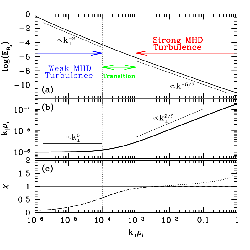
Figure 2: Results of the weakened cascade model for the transition from weak MHD turbulence to strong MHD turbulence for a plasma with $\beta_{i}=1$ and $T_{i}/T_{e}=1$. Plotted in the panels are: (a) the logarithm of the energy spectrum of the perpendicular magnetic field fluctuations, $\log(E_{B_{\perp}})=\log(b_{k}^{2}/k_{\perp})$, normalized by the value of the spectrum at the driving scale, (b) the normalized parallel wavenumber $k_{\parallel}\rho_{i}$, and (c) the nonlinearity parameter $\chi$ vs. the normalized perpendicular wavenumber $k_{\perp}\rho_{i}$. Results show a weak MHD turbulence regime for $k_{\perp}\rho_{i}\in[10^{-6},10^{-4}]$, a transition regime for $k_{\perp}\rho_{i}\in[10^{-4},10^{-3}]$, and a strong MHD turbulence regime for $k_{\perp}\rho_{i}\in[10^{-3},1]$.

Given that the state of the art in numerical simulations of turbulence can reach only a factor of approximately $10^{3}$ in each dimension, these results would suggest that it is not currently possible to capture the physics of the transition from the weak to the strong MHD turbulence regime in a single numerical simulation. Since the transition regime spreads over a factor of 10 in dynamic range, and one would need a minimum dynamic range of 10 in each of the weak and the strong turbulence regimes, these ranges alone would require all of the resolution currently feasible, leaving no room for energy injection and dissipation. Recent work simulating sub-ranges of this plot, however, have indeed confirmed the transition from the weak to the strong scaling of the magnetic energy spectrum in a series of reduced MHD simulations Perez:2008 .

V.2 Local vs. Nonlocal Models

To test the importance of the nonlocal contribution to the turbulent energy cascade rate, we can define a comparable local model by defining the nonlinear frequency at a given perpendicular wavenumber,

$$\omega_{nl}(k_{\perp})=C_{3}\omega_{nl}^{(\mbox{loc})}(k_{\perp}).$$ (31)

Note that the constant $C_{3}$ does not represent an additional free parameter for this local model—this constant may be absorbed into the Kolmogorov constant $C_{1}$—but is introduced to enable easy comparison with the nonlocal model given by equation (26). The integration of equation (26) in the strong MHD and strong KAW inertial ranges (when damping is negligible), as presented in Appendix A, suggest that, to yield comparable local and nonlocal models, the value of this constant should be set to $C_{3}=2.25$; in this case, the values of $C_{1}$ and $C_{2}$ in the local and nonlocal models should be directly comparable. We shall see below that, although the local model can fit nonlinear numerical simulation results in certain circumstances, it is missing the essential physics required to fit a wide range of cases.

In evaluating the nonlocal model, it is desirable to determine the relative contributions of large-scale shearing, local scale motions, and small-scale diffusion to the nonlinear frequency at particular wavenumber, $\omega_{nl}(k_{\perp})$. If the definition of the local contribution given in equation (22) is used, the delta function ensures that the local contribution is an infinitesimal slice of the entire integral, and the local contribution is not easily comparable to the large- or small-scale contributions. To yield more easily interpretable results for the contributions to $\omega_{nl}(k_{\perp})$, we split the integral in equation (26) into three ranges: the large-scale shearing contribution (s) over $[k_{\perp 0},k_{\perp}/2)$, the local-scale contribution (l) over $[k_{\perp}/2,2k_{\perp}]$, and the small-scale diffusive contribution (d) over $(2k_{\perp},k_{\perp max}]$.

Although the weakened cascade model follows only the cascade of perpendicular magnetic energy, the energy spectra of other fields can be constructed from the stready-state solution. Assuming the waves have the character of the linear Alfvénic eigenmodes, we use the solution of the linear kinetic eigenfunction as a function of $k_{\perp}$ to construct, for example, the amplitude of the perpendicular electric field fluctuation from the amplitude of the perpendicular magnetic field fluctuation given by the cascade model solution. Because the phase and amplitude relations between the fields are fixed by the linear kinetic physics, no additional free parameters are introduced: if the linear character of the fluctuations applies, the solution of the perpendicular magnetic energy spectrum determines the energy spectra of the other fields. This linearity assumption appears to be well satisfied in comparisons to nonlinear kinetic simulation results Howes:2008a . This approach enables us to fit three different curves by adjusting only the two Kolmogorov constants, $C_{1}$ and $C_{2}$, in the weakened cascade model, providing increased confidence in fits to numerical spectra.

V.2.1 Moderately Damped $\beta_{i}=1$ Case

The first comparison of the local and nonlocal weakened cascade models tests their ability to fit the results of the $\beta_{i}=1$ dissipation range simulation, the first kinetic simulation resolving both the ion and electron Larmor radius scales in a single simulation, the full details of which are reported in a companion paper Howes:2011a . The plasma parameters for this gyrokinetic simulation using AstroGK Numata:2010 are $\beta_{i}=1$ and $T_{i}/T_{e}=1$, and all dissipation is provided by physically resolved collisionless damping via the Landau resonance onto the ions and electrons. In Figure 3 are plotted the one-dimensional energy spectra (thick lines) for the perpendicular magnetic field fluctuations $E_{B_{\perp}}$ (black solid), the parallel magnetic field fluctuations $E_{B_{\parallel}}$ (magenta dot-dashed), and the perpendicular electric field fluctuations $E_{E_{\perp}}$ (green dashed).

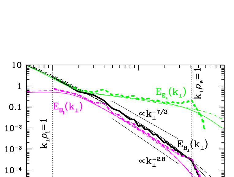
Figure 3: Energy spectra from the $\beta_{i}=1$ dissipation range simulation Howes:2011a resolving both the ion and electron Larmor radius scales, depicted by vertical dotted lines. For a $\beta_{i}=1$ and $T_{i}/T_{e}=1$ plasma, thick lines present numerical energy spectra for the perpendicular magnetic (black solid), electric (green dashed), and parallel magnetic (magenta dot-dashed) fields. Predicted energy spectra from the nonlocal model (thin solid) for $C_{1}=1.65$ and the local model (thin dashed) for $C_{1}=1.8$ are overplotted for comparison.

For comparison, the predicted energy spectra from the the nonlocal weakened cascade model (thin solid) and the local cascade model (thin dashed) are overplotted on Figure 3. Using the linear gyrokinetic eigenfunctions for the Alfvén mode enables the determination of the parallel magnetic and perpendicular electric field spectra from the perpendicular magnetic spectrum output by the cascade model. For the nonlocal model, the Kolmogorov constants required to yield a good fit to the numerical simulation results are $C_{1}=1.65\pm 0.20$ and $C_{2}=1.0$, while for the local model they are $C_{1}=1.8\pm 0.35$, $C_{2}=1.0$, and $C_{3}=2.25$. Note that a higher value of $C_{1}$ leads to stronger weighting of the linear damping relative to the nonlinear energy transfer. The Kolmogorov constant $C_{1}$ is the primary adjustable parameter in the weakened cascade model, dominantly controlling the shape of the energy spectrum. The second Kolmogorov constant $C_{2}$ fine tunes the condition of critical balance, and has not been adjusted; tests of the distribution of energy in wavevector space are necessary to constrain this Kolmogorov constant and are beyond the scope of the present work.

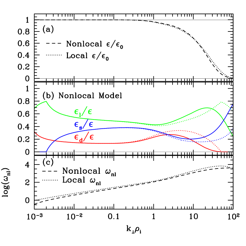
Figure 4: From the local and nonlocal weakened cascade models for the $\beta_{i}=1$ and $T_{i}/T_{e}=1$ plasma depicted in Figure 3, (a) the energy cascade rate $\epsilon/\epsilon_{0}$ vs. $k_{\perp}\rho_{i}$ for local (dotted) and nonlocal (dashed) models, (b) the fractional contribution to $\epsilon$ due to the large-scale shearing motions $\epsilon_{s}/\epsilon$ (blue), the local-scale motions $\epsilon_{l}/\epsilon$ (green), and the small-scale diffusive motions $\epsilon_{d}/\epsilon$ (red) with linear kinetic damping (solid) and with no damping (dotted), and (c) the nonlinear frequency $\omega_{nl}$ from the local model (dotted) and the nonlocal model (dashed).

Comparison of the energy spectra indicates that both the nonlocal and local cascade models are able to reproduce the $\beta_{i}=1$ simulation spectra with similar values for $C_{1}$. Differences between the models become clear as we look more closely at various contributions to the energy cascade rate, as presented in Figure 4. In panel (a), the energy cascade rate $\epsilon$ is plotted vs. $k_{\perp}\rho_{i}$ for local (dotted) and nonlocal (dashed) models. This comparison shows little difference between models, so we must look more closely at the local and nonlocal contributions to the energy cascade rate.

In panel (b) of Figure 4, for the nonlocal model, the fractions of the energy cascade rate from the large-scale shearing motions $\epsilon_{s}/\epsilon$ (blue), the local-scale motions $\epsilon_{l}/\epsilon$ (green), and the small-scale diffusive motions $\epsilon_{d}/\epsilon$ (red) are plotted. To highlight the effects of kinetic dissipation on these contributions to the energy cascade rate, dotted lines give the results when kinetic dissipation is artificially set to zero. From this plot, it is clear that, as the cascade proceeds to higher wavenumber, the diffusive contribution (red) to the cascade diminishes first at $k_{\perp}\rho_{i}\sim 1$ due to dissipation (compared to the undamped case given by the red dotted line), leading to a fractional increase in the local and shear contributions. Next, the fraction of $\epsilon$ due to local motions (green) begins to diminish at around $k_{\perp}\rho_{i}\sim 20$, leading eventually to a dominance of the energy cascade rate by the shearing motions of the large scales (blue). It is this dominance of the energy cascade rate by the large scale motions as kinetic damping dissipates the turbulent motions that is the primary difference between the local and nonlocal models. Note that the unusual peak at the left for $\epsilon_{l}/\epsilon$ is due to the window that defines the local contributions Note3 .

The difference between the local and nonlocal models can be seen at high wavenumbers in the nonlinear frequency $\omega_{nl}$, plotted in panel (c). For the local model (dotted), the nonlinear frequency peaks at around $k_{\perp}\rho_{i}\sim 50$, and then begins to diminish due to the dissipation of the local motions responsible for the nonlinear energy transfer. The nonlocal model (dashed), on the other hand, merely flattens out, as large scale motions continue to support the nonlinear energy transfer at smaller scales.

In summary, both the local and nonlocal models yield similar results in modeling the turbulent energy spectra in the moderately damped $\beta_{i}=1$ case, as shown in Figure 3. The differences become apparent only as the kinetic dissipation becomes sufficiently strong to diminish the local contribution to the nonlinear energy transfer, enabling nonlocal, large-scale shearing motions to dominate the nonlinear frequency, as seen at the high $k_{\perp}\rho_{i}$ end of panel (b) in Figure 4. It is this difference in the physical mechanisms that will prove crucial in cases where the kinetic damping is stronger, requiring the additional physics of the effect of nonlocal motions on the energy transfer to model correctly the steady-state energy spectra.

V.2.2 Strongly Damped $\beta_{i}=0.01$ Case

In a low beta plasma, the kinetic damping of fluctuations in the KAW regime is substantially stronger. In this more strongly damped case, the difference between the local and nonlocal models is dramatic: the local model is simply unable to fit the shape of the spectrum. In this section we compare the spectra predicted by the local and nonlocal cascade models to the steady state of the $\beta_{i}=0.01$ nonlinear AstroGK simulation. In Figure 5, panel (a) shows a fit of the nonlocal model to the AstroGK simulation spectra (same legend as Figure 3), using $C_{1}=2.85$ (thin solid) and with $C_{1}=2.85\pm 0.15$ (thin dashed). In panel (b) is presented the best fit using the local cascade model, for $C_{1}=2.6$ (thin solid) and $C_{1}=2.6\pm 0.4$ (thin dashed). All cascade models in this figure use $C_{2}=1$ and, as usual, the local model employs $C_{3}=2.25$ so that the Kolmogorov constants of both models are comparable. It is immediately apparent that the local model is incapable of fitting the correct shape of the spectrum, generally showing power law slopes that are too flat at the low wavenumbers and a cutoff that is too sharp at high wavenumbers; the neglect of the effect of nonlocal motions on the energy cascade rate at high wavenumbers, where the kinetic dissipation becomes strong, leads to this failure of the local model.

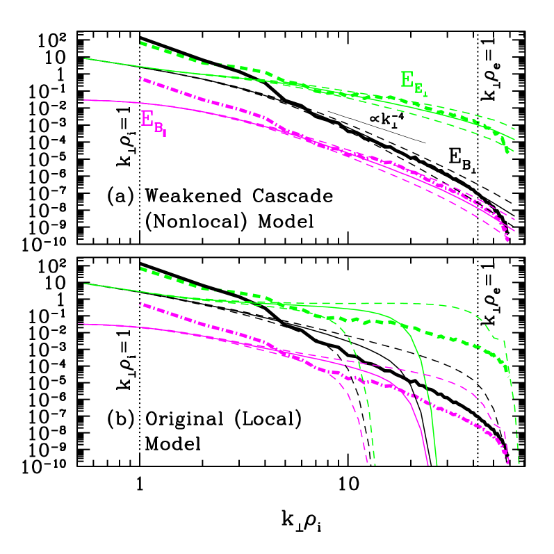
Figure 5: Energy spectra from the nonlinear AstroGK gyrokinetic simulation of turbulence in a plasma with $\beta_{i}=0.01$ and $T_{i}/T_{e}=1$. Thick lines represent numerical energy spectra for the perpendicular magnetic (black solid), electric (green dashed), and parallel magnetic (magenta dot-dashed) fields. (a) The nonlocal model with $C_{1}=2.85\pm 0.15$, where thin solid lines are the spectra for the central value, and the dashed lines demonstrate the $\pm 0.15$ variation. (b) The local model with $C_{1}=2.6\pm 0.4$.

An inspection of the nonlinear frequency $\omega_{nl}$ for both models, plotted in Figure 6, further illustrates this point. The nonlinear frequency for the local model (dotted) peaks at about $k_{\perp}\rho_{i}\simeq 6$, and then drops off rapidly. This occurs because strong kinetic damping dissipates the turbulent fluctuations at the local scale, consequently slowing the nonlinear energy transfer due to those local motions and enabling the linear kinetic damping to dominate over energy transfer at that scale, resulting in a sharp cutoff of the turbulent energy spectra. The nonlocal model (dashed), on the other hand, shows that the nonlinear frequency flattens to a constant value at high wavenumbers but does not decrease. In this case, it is the nonlocal, large-scale shearing motions Note4 . that dominate the nonlinear energy transfer rate at high wavenumbers, leading to turbulent spectra that do not cut off sharply and are able to fit the nonlinear numerical results. This evidence suggests that it is the effect of nonlocal motions on the nonlinear energy transfer rate that is responsible for the more slowly dissipating, nearly power-law appearance of the turbulent spectra in both recent solar wind observations Sahraoui:2009 ; Kiyani:2009 ; Alexandrova:2009 ; Chen:2010 ; Sahraoui:2010b and nonlinear numerical simulations Howes:2011a .

Figure 6: The nonlinear frequency $\omega_{nl}$ for the local (dotted) and nonlocal (dashed) cascade models for the $\beta_{i}=0.01$ and $T_{i}/T_{e}=1$ turbulent plasma shown in Figure 5.

In summary, although the local model can fit the data in certain moderately damped cases, the effect of nonlocal, large-scale shearing motions on the nonlinear energy transfer deep in the dissipation range is essential to avoid a sharp cutoff of the spectra and fit the nearly power-law behavior observed in both solar wind observations and nonlinear numerical simulations

V.2.3 Weak Dissipating KAW Turbulence (WDKT)

A graphical depiction of the contribution of nonlocal turbulent fluctuations to the energy cascade rate at a particular wavenumber $k_{\perp}$ illuminates the effect of nonlocality. Here the weakened cascade model, defined in §III.3, is used to solve for the steady state of a plasma with $\beta_{i}=1$ and $T_{i}/T_{e}=16$, parameters chosen so that there is a sufficient dynamic range of the kinetic Alfvén wave regime to realize the asymptotic limit of the undamped KAW cascade before reaching $k_{\perp}\rho_{e}\sim 1$ at $k_{\perp}\rho_{i}\sim 170$. The model covers a range of wavenumbers $k_{\perp}\rho_{i}\in[10^{-3},10^{3}]$, employs constants $C_{1}=4.5$ and $C_{2}=1$, and is driven in critical balance with $\chi(k_{\perp 0})=1$. In Figure 7, the perpendicular magnetic energy spectrum $E_{B_{\perp}}$ in panel (a) reveals a strong MHD turbulence regime over $k_{\perp}\rho_{i}\in[10^{-3},1]$ and a strong KAW turbulence regime over $k_{\perp}\rho_{i}\in[1,10^{2}]$. The kinetic dissipation begins to significantly alter the spectra for $k_{\perp}\rho_{i}\gtrsim 100$, leading to a transition from strong to weak turbulence locally. But this situation is not a standard weak turbulence picture, such as those typically considered in incompressible MHD turbulence. Rather, the presence of large-scale shearing motions and the importance of further kinetic dissipation leads to a very different kind of weak KAW turbulence: we refer to this as the range of weak dissipating KAW turbulence (WDKT), seen over wavenumbers $k_{\perp}\rho_{i}\in[10^{2},10^{3}]$ in panel (a) of Figure 7.

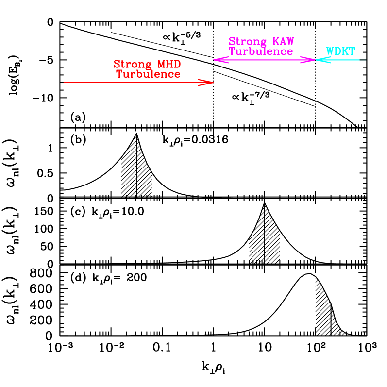
Figure 7: (a) The perpendicular magnetic energy spectrum for strong turbulence in a plasma with $\beta_{i}=1$ and $T_{i}/T_{e}=16$ predicted by the weakened cascade model. In the three lower panels is plotted the function in the integrand of equation (26) for the total nonlinear frequency $\omega_{nl}(k_{\perp})$ at (b) $k_{\perp}\rho_{i}=0.0316$, (c) $k_{\perp}\rho_{i}=10$, and (d) $k_{\perp}\rho_{i}=200$. The value of the local wavenumber $k_{\perp}$ is indicated in each plot by the vertical solid line, and shading represents contributions due to motions on local scales from $k_{\perp}/2$ to $2k_{\perp}$.

Plotted in the lower three panels of Figure 7 is the function in the integrand of equation (26) for the total nonlinear frequency $\omega_{nl}(k_{\perp})$ at (b) $k_{\perp}\rho_{i}=0.0316$, (c) $k_{\perp}\rho_{i}=10$, and (d) $k_{\perp}\rho_{i}=200$, where the value of local wavenumber $k_{\perp}$ is indicated in each plot by the vertical solid line. The contributions to the integral yielding $\omega_{nl}(k_{\perp})$ due to local motions is given by the shaded region below the curve (from $k_{\perp}/2$ to $2k_{\perp}$); below the curve at lower wavenumbers is the contribution from large-scale shearing motions, and at higher wavenumbers, from small-scale diffusive motions. In panel (b) is the contribution to the nonlinear frequency at $k_{\perp}\rho_{i}=0.0316$ in the strong MHD turbulence regime. The nonlinear frequency in this regime is dominated by local motions, with large-scale shearing contributing slightly more than small-scale diffusive motions. In panel (c) is the contribution to the nonlinear frequency at $k_{\perp}\rho_{i}=10$ in the strong KAW turbulence regime. Again, $\omega_{nl}(k_{\perp})$ is dominated by local motions, and here small-scale diffusive motions contribute slightly more than large-scale shearing. In panel (d) is highlighted one of the key physics points of the weakened cascade model: the nonlinear frequency at $k_{\perp}\rho_{i}=200$ in the weak dissipating KAW turbulence regime is dominated by large-scale shearing motions and not by local scale motions. Additionally, there is no contribution from small-scale diffusion because the cascade is terminated and no motions exist at smaller scales.

V.3 Complete Spectrum

The power of the weakened cascade model is best summarized by a single final example that demonstrates all of the physics incorporated, including the transition from weak to strong MHD turbulence and the complementary transition from strong KAW to weak dissipating KAW turbulence. This case models the entire turbulent cascade over $k_{\perp}\rho_{i}\in[10^{-5},300]$ for a $\beta_{i}=1$ and $T_{i}/T_{e}=9$ plasma with weak energy injection $\chi(k_{\perp 0})=0.1$ at $k_{\perp 0}\rho_{i}=k_{\parallel 0}\rho_{i}=10^{-5}$. The Kolmogorov constants are $C_{1}=1.4$ and $C_{2}=1.0$.

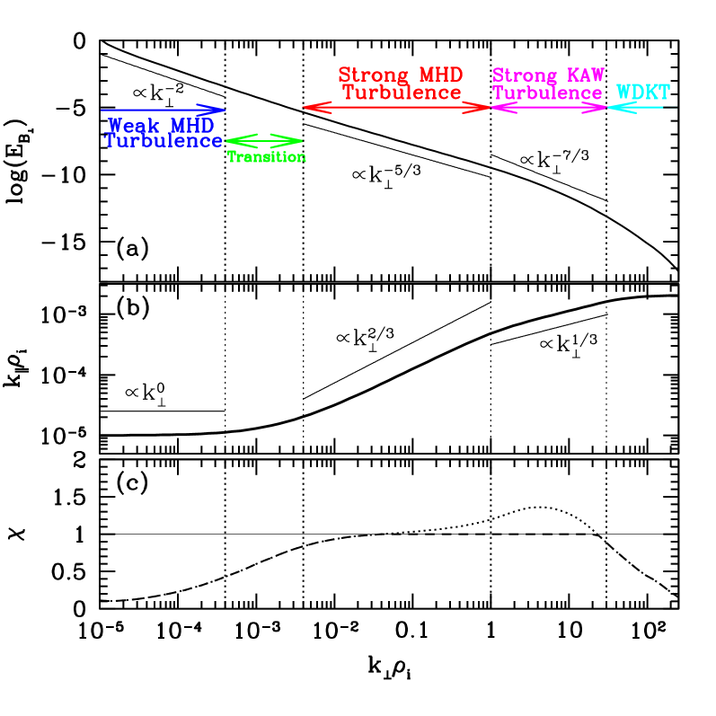
Figure 8: Numerical solution of the weakened cascade model for the steady state spectrum in a $\beta_{i}=1$ and $T_{i}/T_{e}=9$ plasma. The panels plotted are the same as Figure 2. Regimes indicated in panel (a) are weak MHD turbulence, a transition regime from weak to strong MHD turbulence, strong MHD turbulence, strong KAW turbulence, and finally weak dissipating KAW turbulence (WDKT).

The steady-state perpendicular magnetic energy spectrum $E_{B_{\perp}}$ for this case is presented in panel (a) of Figure 8. Panel (b) contains the evolution of the parallel wavenumber $k_{\parallel}\rho_{i}$ and panel (c) shows the evolution of the nonlinearity parameter $\chi$ over the entire cascade. The solution shows weak MHD turbulence over the range $k_{\perp}\rho_{i}\in[10^{-5},4\times 10^{-4}]$, with a one-dimensional magnetic energy spectrum $E_{B_{\perp}}\propto k_{\perp}^{-2}$, no parallel cascade, and weak nonlinearity $\chi<0.5$. Then comes a regime of transition from weak to strong MHD turbulence in the range $k_{\perp}\rho_{i}\in[4\times 10^{-4},4\times 10^{-3}]$. Over $k_{\perp}\rho_{i}\in[4\times 10^{-3},1]$ is strong MHD turbulence with spectrum $E_{B_{\perp}}\propto k_{\perp}^{-5/3}$, parallel cascade scaling as $k_{\parallel}\propto k_{\perp}^{2/3}$ according to critical balance, and a nonlinearity parameter $\chi\sim 1$. The transition from strong MHD turbulence to strong KAW turbulence occurs at $k_{\perp}\rho_{i}\sim 1$. The range of strong KAW turbulence over $k_{\perp}\rho_{i}\in[1,30]$ yields a spectrum $E_{B_{\perp}}\propto k_{\perp}^{-7/3}$, parallel cascade scaling as $k_{\parallel}\propto k_{\perp}^{1/3}$ according to critical balance, and a nonlinearity parameter $\chi\sim 1$. Finally as the kinetic dissipation begins to become significant, the cascade becomes weak dissipating KAW turbulence (WDKT) over $k_{\perp}\rho_{i}\in[30,300]$, with a spectrum that drops off exponentially, inhibition of the parallel cascade, and a dropping nonlinearity parameter $\chi<1$.

VI Discussion

The weakened cascade model, summarized in §III.3, is a refinement of an earlier cascade model Howes:2008b intended to explain better the spectra observed in nonlinear numerical simulations Howes:2011a and recent high time resolution observations of the dissipation range of turbulence in the near Earth solar wind Sahraoui:2009 ; Kiyani:2009 ; Alexandrova:2009 ; Chen:2010 ; Sahraoui:2010b . The new physical effects incorporated into this model are (1) the transition between weak and strong turbulence and (2) the effect on the nonlinear turbulent energy transfer by nonlocal fluctuations.

The model is constructed to have as few free parameters as possible, letting the linear physics of the kinetic plasma dictate the character of the turbulent fluctuations. The weakened cascade model has only two free parameters in the form of dimensionless, order-unity Kolmogorov constants: $C_{1}$, which adjusts the weighting of the nonlinear energy transfer to the linear kinetic damping, and $C_{2}$, which fine tunes the condition of critical balance in the nonlinearity parameter $\chi$. To determine a value of $C_{2}$ from numerical simulations or observations is beyond the scope of the present work, so in all cases we have set $C_{2}=1$, essentially leaving only a single adjustable parameter $C_{1}$ to determine the shape of the steady-state energy spectra. As presented in §V, this single degree of freedom in the weakened cascade model is sufficient to fit closely the shape of the turbulent spectra from nonlinear gyrokinetic simulations for both moderately damped $\beta_{i}=1$ and strongly damped $\beta_{i}=0.01$ cases, giving us confidence that the model contains the essential ingredients necessary to describe successfully the energetics of the turbulent cascade in a weakly collisional plasma.

Two novel ingredients, inspired by turbulence phenomenology, are central to the weakened cascade model. The first is the prescription for the evolution of the parallel cascade depending on the strength of the nonlinearity parameter, given by equation (30). This equation is constructed to reproduce the predictions of strong and weak turbulence theories in the appropriate limits. The second, and likely more important, ingredient is the nonlocal form of the nonlinear energy transfer frequency, given by equation (26). The abandonment of the Kolmogorov hypothesis of locality Kolmogorov:1941 is the advance necessary to explain the nearly power-law spectra seen in both the nonlinear simulation results Howes:2011a and the solar wind dissipation range observations Sahraoui:2009 ; Kiyani:2009 ; Alexandrova:2009 ; Chen:2010 ; Sahraoui:2010b . When dissipation begins to weaken the local scale motions, the smaller scale motions are necessarily yet more strongly damped, so diffusion by those smaller scale motions is effectively negligible. Therefore, the key result of the weakened cascade model presented here is that the nonlocal effect of shearing by large scale motions explains the nearly power law appearance of numerical and observational spectra in the dissipation range (this effect is particularly critical in the low beta case presented in §V.2.2).

The locality of MHD turbulence in the inertial range has gained a significant amount of attention in the literature recently, with some studies finding evidence for nonlocality Schekochihin:2004d ; Alexakis:2005 ; Carati:2006 ; Yousef:2007 , while other studies claim locality in the asymptotic limit of large Reynold’s numbers Aluie:2010 (see Mininni 2010 Mininni:2010 for a recent review of this topic). At question is whether the properties of the MHD inertial range become independent of the details of the mechanisms responsible for driving and dissipating the turbulence, enabling the determination of a self-similar solution for a universal MHD turbulent spectrum. When the dissipation range of plasma turbulence is being considered, however, it is obvious that no self-similar solution can be found, so the importance of a nonlocal contribution to the energy cascade rate in the dissipation range, as proposed here, should come as no surprise.

It is interesting to note that scale locality would be recovered, and therefore a self-similar solution would arise, if the kinetic Alfvén wave range of scales, $\rho_{i}\ll 1/k\ll\rho_{e}$, becomes asymptotically large, as occurs in the limit of vanishing electron mass, $m_{e}\rightarrow 0$. In this very small electron mass limit $m_{e}\rightarrow 0$, the kinetic Alfvén wave parallel phase velocity is always much less than the electron thermal velocity, $\omega/k_{\parallel}\ll v_{te}$, so collisionless damping via resonant wave-particle interactions with the electrons becomes negligible. In the absence of damping, a second inertial range is recovered for the dispersive kinetic Alfvén waves over the range of scales $\rho_{i}\ll 1/k\ll\rho_{e}$. The weakened cascade model describes this limit correctly, because if $m_{e}\rightarrow 0$, then the collisionless damping rate $\gamma\rightarrow 0$ in equation (13). In this case, the weakened cascade model recovers a second inertial range of kinetic Alfvén waves with a spectral index of $-7/3$, as shown by the dashed line denoted the “undamped model” in Figure 3 of the original cascade model paper by Howes et al. (2008) Howes:2008b .

VI.1 Comparison to Previous Cascade Models

It is instructive to compare the predictions of the weakened cascade model, with its inclusion of nonlocal effects on the energy cascade rate, to those of the original cascade model Howes:2008b and of a similar model by Podesta et al. 2010Podesta:2010a , both strictly local models. Two of the general conclusions of the original cascade model were that variations in collisionless damping with plasma parameters naturally explained observed variations in solar wind turbulent spectra and that the dissipation range spectrum should be an exponential fall off Howes:2008b . Podesta et al. make the stronger claim that “an energy cascade consisting solely of KAWs cannot reach scales of order the electron gyroradius, $k_{\perp}\rho_{e}\sim 1$. It implies that the power-law spectrum in the regime of electron scales must be supported by wave modes other than the KAW” Podesta:2010a .

Since the only wave mode supported in the dissipation range of a $\beta_{i}=1$ plasma in gyrokinetic theory is the kinetic Alfvén wave, the $\beta_{i}=1$ gyrokinetic simulation Howes:2011a demonstrates unequivocally by counterexample that the claim by Podesta et al. Podesta:2010a —that the kinetic Alfvén wave cascade cannot reach scales $k_{\perp}\rho_{e}\sim 1$—is incorrect. We explain below that the primary reason for this failure lies in the determination of the Kolmogorov constant in their cascade model.

Each of these cascade models incorporates an order-unity dimensionless constant that essentially adjusts the weighting of nonlinear energy transfer to that of the linear kinetic damping. Podesta et al. estimate $k_{\perp}\rho_{i}\simeq 28$ as the wavenumber at which the KAW cascade terminates, given by their equation (23), which is linearly dependent on their constant $A$. Without any guidance to determine this constant, Podesta et al. base their conclusions on the theory with $A=1$. We can usefully compare their model with the local version of the weakened cascade model (using equation [31] for the nonlinear frequency) to determine what value of $A$ would fit the $\beta_{i}=1$ dissipation range simulation spectra in Figure 3. Using $b_{k}^{2}=kE(k)$ in the limit $k_{\perp}\gg k_{\parallel}$ to connect to their model, the energy cascade rate $\epsilon$ in our local model is given by

$$\epsilon=C_{1}^{-3/2}C_{3}\omega_{nl}^{(\mbox{loc})}kE(k).$$ (32)

The energy cascade rate $\varepsilon$ in Podesta et al., based on their equation (6) Note5 , is given by

$$\varepsilon=\frac{A}{2\pi}\omega kE(k).$$ (33)

The assumption of critical balance is taken by Podesta et al. to be $\omega=\omega_{nl}^{(\mbox{loc})}$, so the two models should give similar results if $A=2\pi C_{1}^{-3/2}C_{3}$. Substituting in the best fit values $C_{1}=1.8$ and $C_{3}=2.25$ from Figure 3, we find $A=5.85$. This comparison suggests that Podesta et al. significantly underestimated the weight of the energy cascade rate relative to the linear kinetic damping, leading to a conclusion inconsistent with direct numerical simulations of kinetic turbulence. Nonlinear kinetic simulations of turbulence therefore play an invaluable role in the effort to understand turbulence in the solar wind and other weakly collisional astrophysical plasmas.

VI.2 Limitations of the Weakened Cascade Model

The weakened cascade model has been developed to predict the turbulent energy spectra occurring in weakly collisional astrophysical plasmas. We discuss here a number of assumptions that have been made in the construction of the model.

First, the model has been constructed to reproduce the scaling of the turbulent energy spectra given by the Goldreich and Sridhar theories for weak and strong MHD turbulence Sridhar:1994 ; Goldreich:1995 ; Lithwick:2003 , and their extension to turbulence in the kinetic Alfvén wave regime. An alternative theory for the scaling of strong MHD turbulence has been proposed by Boldyrev Boldyrev:2006 , and substantial numerical support has accumulated in its favor Mason:2006 ; Mason:2008 ; Perez:2008 ; Boldyrev:2009 ; Perez:2009 ; Perez:2010. Modifications of the weakened cascade model to reproduce instead the Bolydrev scalings will be discussed in a subsequent paper.

Another potential limitation of the weakened cascade model is the conjecture that the parallel cascade of energy is inhibited for weak turbulence in both the MHD and KAW regimes, as discussed in §III.1.

The one-dimensional nature of the weakened cascade model restricts its direct applicability to plasmas in which there is a single scale of energy injection at the outer scale $(k_{\perp 0},k_{\parallel 0})$. As discussed in Howes et al. 2008 Howes:2008b , the lack of structure at small scales in the solar wind energy spectrum is evidence against significant energy injection as scales smaller than the outer scale $(k_{\perp 0},k_{\parallel 0})$, so the model appears to be broadly applicable to the solar wind.

A number of other factors that may significantly affect the turbulent fluctuations in the solar wind are not incorporated into the weakened cascade model, including the radial expansion of the solar wind, kinetic temperature anisotropy instabilities, and the imbalance of sunward and anti-sunward Alfvén wave energy fluxes. A detailed discussion of these effects is presented in the paper describing the original cascade model Howes:2008b and will not be repeated here. It suffices to say that the weakened cascade model is an attempt to understand the quantitative details of the energy transport in balanced, Alfvénic turbulence in a weakly collisional plasma; the relation of these additional effects to this fundamental turbulent evolution merits further investigation.

The weakened cascade model does not account for one recently discovered physical mechanism that may play an important role in the energy transport in weakly collisional Alfvénic turbulence: the entropy cascadeSchekochihin:2009 ; Tatsuno:2009 ; Plunk:2010 ; Tatsuno:2010 ; Plunk:2011 . As described in Schekochihin et al. 2009 Schekochihin:2009 , the ion entropy cascade is a dual cascade to small scales in both physical space and velocity space of the ion distribution function. Operating at scales below the ion Larmor radius $k_{\perp}\rho_{i}>1$, in the regime of kinetic Alfvén wave turbulence, this process is driven by nonlinear phase mixing and represents an alternative channel of energy transport that is not included in the weakened cascade model. Comparisons of the predictions of the weakened cascade model with the results of a suite of nonlinear gyrokinetic simulations will enable an evaluation of the importance of the ion entropy cascade in the turbulent energy transport, an important line of future research.

VII Conclusions

Early cascade models for kinetic turbulence in weakly collisional astrophysical plasmas, such as the solar wind, suggested that the energy spectra in the dissipation range should exponentially fall off Howes:2008b , and that due to collisionless damping, kinetic Alfvén waves could not be responsible for the cascade of energy to electron scales Podesta:2010a . However, nonlinear kinetic simulations of turbulence over the entire dissipation range Howes:2011a and high time resolution observations of the dissipation range fluctuations in the solar wind Sahraoui:2009 ; Kiyani:2009 ; Alexandrova:2009 ; Chen:2010 ; Sahraoui:2010b yield nearly power-law energy spectra rather than an exponential decay. The failure of these early cascade models motivated refinements to explain the numerical and observational results, yielding the weakened cascade model presented here.

The original cascade model by Howes et al. 2008Howes:2008b was based on three assumptions: (1) the Kolmogorov hypothesis of the locality of the nonlinear energy transfer in wavenumber space, (2) the conjecture of critical balance at all scales, and (3) the applicability of linear kinetic damping rates. The weakened cascade model eliminates the first two assumptions of the original model, resulting in a more broadly applicable and physically realistic model.

The assumption of critical balance at all scales is dropped; instead, the model handles explicitly the transition between weak and strong turbulence. A key point in the treatment of weak turbulence is our conjecture that the parallel cascade is inhibited in both the MHD and kinetic Alfvén wave regimes. This physics is contained in the model for the evolution of the parallel wavenumber given by equation (30). The more significant advance of the weakened cascade model is the abandonment of the locality hypothesis of Kolmogorov. Although energy is still transferred locally in wavenumber space—for example, from $k_{\perp}$ to $2k_{\perp}$—the turbulent fluctuations responsible for that energy transfer may be nonlocal. Both shearing by motions at larger scales and diffusion by motions at smaller scales contribute to the nonlinear energy cascade rate according to equation (26).

In §V, we have demonstrated that the weakened cascade model reproduces the transition from weak to strong MHD turbulence as predicted by theory. As the collisionless dissipation in the kinetic Alfvén wave regime becomes significant, the model also shows a complementary transition from strong KAW turbulence to weak dissipating KAW turbulence, a new regime of weak turbulence in which the effect of shearing by large scale motions and continued kinetic dissipation play an important role.

The key result of this paper is that the nearly power-law energy spectra observed in the dissipation range of both numerical simulations and solar wind observations are explained by the inclusion of the effect of nonlocal motions on the nonlinear energy cascade rate, specifically the shearing by large-scale motions. Although numerical spectra for a moderately damped $\beta_{i}=1$ plasma may be equally well explained by either local or nonlocal models (Figure 3), for the more strongly damped $\beta_{i}=0.01$ plasma, the inclusion of nonlocal effects is critical for the model to fit the numerical energy spectra (Figure 5). The importance of the nonlocal shearing motions to the energy cascade rate is demonstrated in panel (d) of Figure 7, where it is clear that the large-scale contribution dominates over the local contribution. The effect at these strongly dissipative scales is that the nonlinear frequency does not decrease with increasing perpendicular wavenumber, as a local model would suggest, but that it remains constant due to the large-scale contribution, as shown in Figure 6. Thus, by abandoning the Kolmogorov hypothesis of locality, the weakened cascade model explains the nearly power-law spectra found in numerical and observational studies of the dissipation range by including the nonlocal effect of large-scale shearing motions on the energy transfer rate.

The ultimate aim of the weakened cascade model is not to fit numerical and observational turbulent spectra, but to predict them. Nonlinear kinetic simulations of dissipation range turbulence have already played an important role in evaluating the weakened cascade model. Since the Kolmogorov constants $C_{1}$ and $C_{2}$ may, in principle, depend on the plasma parameters $\beta_{i}$ and $T_{i}/T_{e}$, numerical studies will continue to play a critical role as we perform a suite of kinetic turbulence simulations over a range of plasma parameters to determine this dependence, ultimately striving for predictive capability. In addition, these numerical studies will also be crucial in judging the importance of the ion entropy cascade to the turbulent energy transfer in the dissipation range.

Appendix A The Effect of Nonlocal Interactions on Turbulence Scaling

Here we consider the effect of the nonlocal contribution to the nonlinear frequency, given by equation (26), on the scaling of the spectra in the strong MHD and strong KAW inertial ranges.

In the strong MHD inertial range, the contribution to the nonlinear frequency due to motions at each wavenumber is $\omega_{nl}^{(\mbox{loc})}=k_{\perp}b_{k}=C_{1}^{1/2}\epsilon^{1/3}k_{\perp}^{2/3}$. Performing the integral in equation (26) to find $\omega_{nl}$, we obtain

$$\omega_{nl}(k_{\perp}) = \frac{3}{2}C_{1}^{1/2}\epsilon^{1/3}\left(k_{\perp}^{2/3}-k_{\perp 0}^{2/3}\right)$$ (34)

$$+ \frac{3}{4}C_{1}^{1/2}\epsilon^{1/3}k_{\perp}^{2}\left(k_{\perp}^{-4/3}-k_{\perp max}^{-4/3}\right),$$

where the first term is due to the large-scale shearing, and the second is due to the small-scale diffusion. The inertial range is defined as the range of scales unaffected by large-scale driving or small-scale dissipation, corresponding to the limit $k_{\perp 0}\ll k_{\perp}\ll k_{\perp max}$. In this limit, the nonlinear frequency simplifies to

$$\omega_{nl}(k_{\perp})=\frac{3}{2}\omega_{nl}^{(\mbox{loc})}+\frac{3}{4}\omega_{nl}^{(\mbox{loc})}=\frac{9}{4}\omega_{nl}^{(\mbox{loc})}(k_{\perp}).$$ (35)

Therefore, within the strong MHD inertial range, the nonlinear model yields a nonlinear frequency of the form $\omega_{nl}(k_{\perp})=C_{3}\omega_{nl}^{(\mbox{loc})}(k_{\perp})$, where the constant is $C_{3}=2.25$. This order-unity constant factor is the only difference between models, so the scaling of the nonlocal model within the strong MHD inertial range will therefore be the same as a local model. Note that the contribution of the large-scale shearing motions is twice that of the small-scale diffusive motions.

In the strong KAW inertial range, we have $\omega_{nl}^{(\mbox{loc})}=k_{\perp}b_{k}k_{\perp}\rho_{i}=C_{1}^{1/2}\epsilon^{1/3}\rho_{i}^{2/3}k_{\perp}^{4/3}$. Performing the integral in equation (26), we find

$$\omega_{nl}(k_{\perp}) = \frac{3}{4}C_{1}^{1/2}\epsilon^{1/3}\rho_{i}^{2/3}\left(k_{\perp}^{4/3}-k_{\perp 0}^{4/3}\right)$$ (36)

$$+ \frac{3}{2}C_{1}^{1/2}\epsilon^{1/3}\rho_{i}^{2/3}k_{\perp}^{2}\left(k_{\perp}^{-2/3}-k_{\perp max}^{-2/3}\right),$$

where the first term is the large-scale contribution and the second is the small-scale contribution. Within the KAW inertial range, we apply the limit $k_{\perp 0}\ll k_{\perp}\ll k_{\perp max}$ to simplify the nonlinear frequency to

$$\omega_{nl}(k_{\perp})=\frac{3}{4}\omega_{nl}^{(\mbox{loc})}+\frac{3}{2}\omega_{nl}^{(\mbox{loc})}=\frac{9}{4}\omega_{nl}^{(\mbox{loc})}(k_{\perp}).$$ (37)

Again, we find that the scaling of the nonlocal model in the strong KAW inertial range will be that same as that of a local models, the only difference being the same constant factor $C_{3}=2.25$. In this case, however, the small-scale diffusive motions contribute twice as much to the nonlinear frequency as the large-scale shearing motions.

References

- (1) P. J. Coleman, Jr., “Turbulence, Viscosity, and Dissipation in the Solar-Wind Plasma,” Astrophys. J. 153, 371–388 (Aug. 1968).
- (2) E. Marsch, “Kinetic Physics of the Solar Wind Plasma,” in Physics of the Inner Heliosphere II. Particles, Waves and Turbulence., edited by E Schwenn, R. andMarsch (Springer-Verlag, Berlin, 1991) pp. 45–133.
- (3) E. Marsch, “Kinetic physics of the solar corona and solar wind,” Living Rev. Solar Phys. 3 (2006), http://www.livingreviews.org/lrsp-2006-1.
- (4) G. G. Howes, “Inertial range turbulence in kinetic plasmas,” Phys. Plasmas 15, 055904 (May 2008).
- (5) G. G. Howes, S. C. Cowley, W. Dorland, G. W. Hammett, E. Quataert, and A. A. Schekochihin, “A model of turbulence in magnetized plasmas: Implications for the dissipation range in the solar wind,” J. Geophys. Res. 113, A05103 (May 2008), arXiv:0707.3147.
- (6) G. G. Howes, S. C. Cowley, W. Dorland, G. W. Hammett, E. Quataert, A. A. Schekochihin, and T. Tatsuno, “Howes et al. Reply:,” Phys. Rev. Lett. 101, 149502 (Oct. 2008).
- (7) A. A. Schekochihin, S. C. Cowley, W. Dorland, G. W. Hammett, G. G. Howes, E. Quataert, and T. Tatsuno, “Astrophysical Gyrokinetics: Kinetic and Fluid Turbulent Cascades in Magnetized Weakly Collisional Plasmas,” Astrophys. J. Supp. 182, 310–377 (May 2009).
- (8) G. G. Howes, W. Dorland, S. C. Cowley, G. W. Hammett, E. Quataert, A. A. Schekochihin, and T. Tatsuno, “Kinetic Simulations of Magnetized Turbulence in Astrophysical Plasmas,” Phys. Rev. Lett. 100, 065004 (Feb. 2008).
- (9) G. G. Howes, J. M. TenBarge, W. Dorland, E. Quataert, A. A. Schekochihin, R. Numata, and T. Tatsuno, “Gyrokinetic simulations of solar wind turbulence from ion to electron scales,” Phys. Rev. Lett. 107, 035004 (Jul 2011).
- (10) F. Sahraoui, M. L. Goldstein, P. Robert, and Y. V. Khotyaintsev, “Evidence of a Cascade and Dissipation of Solar-Wind Turbulence at the Electron Gyroscale,” Phys. Rev. Lett. 102, 231102–+ (Jun. 2009).
- (11) K. H. Kiyani, S. C. Chapman, Y. V. Khotyaintsev, M. W. Dunlop, and F. Sahraoui, “Global scale-invariant dissipation in collisionless plasma turbulence,” Phys. Rev. Lett. 103, 075006 (2009).
- (12) O. Alexandrova, J. Saur, C. Lacombe, A. Mangeney, J. Mitchell, S. J. Schwartz, and P. Robert, “Universality of Solar-Wind Turbulent Spectrum from MHD to Electron Scales,” Phys. Rev. Lett. 103, 165003–+ (Oct. 2009).
- (13) C. H. K. Chen, T. S. Horbury, A. A. Schekochihin, R. T. Wicks, O. Alexandrova, and J. Mitchell, “Anisotropy of Solar Wind Turbulence between Ion and Electron Scales,” Physical Review Letters 104, 255002–+ (Jun. 2010), arXiv:1002.2539 [physics.space-ph].
- (14) F. Sahraoui, M. L. Goldstein, G. Belmont, P. Canu, and L. Rezeau, “Three Dimensional Anisotropic k Spectra of Turbulence at Subproton Scales in the Solar Wind,” Phys. Rev. Lett. 105, 131101–+ (Sep. 2010).
- (15) At spacecraft-frame frequencies above about Hz, in situ measurements of the solar wind one-dimensional magnetic energy frequency spectrum show that the spectrum becomes steeper than the spectral index typically found at lower frequencies Bale:2005 . The range of frequencies at and above this break in the spectrum has traditionally been denoted the dissipation range of solar wind turbulence. In the present work, the dissipation range is interpreted to be associated with the perpendicular scale of the ion Larmor radius, . Other studies have argued for different terminology to describe this range, such as dispersion range Stawicki:2001 or scattering range Rudakov:2011 . Here, we choose to employ the more traditional terminology and denote the range of scales as the dissipation range.
- (16) A. N. Kolmogorov, “The local structure of turbulence in incompressible viscous fluid for very large reynolds numbers,” Dokl. Akad. Nauk SSSR 30, 9– (1941), english Translation: Proc. Roy. Soc. London A, 434, 9 (1991).
- (17) R. S. Iroshnikov, “The turbulence of a conducting fluid in a strong magnetic field,” Astron. Zh. 40, 742 (1963), English Translation: Sov. Astron., 7 566 (1964).
- (18) R. H. Kraichnan, “Inertial range spectrum of hyromagnetic turbulence,” Phys. Fluids 8, 1385–1387 (1965).
- (19) D. C. Robinson and M. G. Rusbridge, “Structure of turbulence in the zeta plasma,” Phys. Fluids 14, 2499–2511 (1971).
- (20) S. J. Zweben, C. R. Menyuk, and R. J. Taylor, “Small-scale magnetic fluctuations inside the macrotor tokamak,” Phys. Rev. Lett. 42, 1270–1274 (1979).
- (21) D. Montgomery and L. Turner, “Anisotropic magnetohydrodynamic turbulence in a strong external magnetic field,” Phys. Fluids 24, 825–831 (1981).
- (22) J. W. Belcher and L. Davis, “Large-Amplitude Alfvén Waves in the Interplanetary Medium, 2,” J. Geophys. Res. 76, 3534–3563 (1971).
- (23) J. V. Shebalin, W. H. Matthaeus, and D. Montgomery, “Anisotropy in mhd turbulence due to a mean magnetic field,” J. Plasma Phys. 29, 525–547 (1983).
- (24) S. Sridhar and P. Goldreich, “Toward a Thoery of Interstellar Turbulence I. Weak Alfvénic Turbulence,” Astrophys. J. 433, 612–621 (1994).
- (25) P. Goldreich and S. Sridhar, “Toward a Thoery of Interstellar Turbulence II. Strong Alfvénic Turbulence,” Astrophys. J. 438, 763–775 (1995).
- (26) D. Montgomery and W. H. Matthaeus, “Anisotropic Modal Energy Transfer in Interstellar Turbulence,” Astrophys. J. 447, 706–+ (Jul. 1995).
- (27) C. S. Ng and A. Bhattacharjee, “Interaction of Shear-Alfven Wave Packets: Implication for Weak Magnetohydrodynamic Turbulence in Astrophysical Plasmas,” Astrophys. J. 465, 845–+ (Jul. 1996).
- (28) P. Goldreich and S. Sridhar, “Magnetohydrodynamic turbulence revisited,” Astrophys. J. 485, 680–688 (1997).
- (29) C. S. Ng and A. Bhattacharjee, “Scaling of anisotropic spectra due to the weak interaction of shear-Alfvén wave packets,” Phys. Plasmas 4, 605–610 (Mar. 1997).
- (30) S. Galtier, S. V. Nazarenko, A. C. Newell, and A. Pouquet, “A weak turbulence theory for incompressible magnetohydrodynamics,” J. Plasma Phys. 63, 447–488 (Jun. 2000), astro-ph/0008148.
- (31) Y. Lithwick and P. Goldreich, “Imbalanced weak magnetohydrodynamic turbulence,” Astrophys. J. 582, 1220–1240 (2003).
- (32) J. C. Perez and S. Boldyrev, “On Weak and Strong Magnetohydrodynamic Turbulence,” Astrophys. J. Lett. 672, L61–L64 (Jan. 2008), arXiv:0712.2086.
- (33) J. C. Higdon, “Density fluctuations in the interstellar medium: Evidence for anisotropic magnetogasdynamic turbulence i. model and astrophysical sites,” Astrophys. J. 285, 109–123 (1984).
- (34) J. Cho and E. T. Vishniac, “The Anisotropy of Magnetohydrodynamic Alfvénic Turbulence,” Astrophys. J. 539, 273–282 (2000).
- (35) J. Maron and P. Goldreich, “Simulations of incompressible magnetohydrodynamic turbulence,” Astrophys. J. 554, 1175–1196 (2001).
- (36) T. S. Horbury, M. Forman, and S. Oughton, “Anisotropic scaling of magnetohydrodynamic turbulence,” Phys. Rev. Lett. 101, 175005 (Oct 2008).
- (37) J. J. Podesta, “Dependence of Solar-Wind Power Spectra on the Direction of the Local Mean Magnetic Field,” Astrophys. J. 698, 986–999 (Jun. 2009), arXiv:0901.4940.
- (38) A. V. Gruzinov, “Radiative Efficiency of Collisionless Accretion,” Astrophys. J. 501, 787–+ (Jul. 1998), astro-ph/9710132.
- (39) E. Quataert and A. Gruzinov, “Turbulence and Particle Heating in Advection-dominated Accretion Flows,” Astrophys. J. 520, 248–255 (Jul. 1999), astro-ph/9803112.
- (40) D. Biskmap, E. Schwarz, A. Zeiler, A. Celani, and J. F. Drake, “Electron magnetohydrodynamic turbulence,” Phys. Plasmas 6, 751–758 (1999).
- (41) J. Cho and A. Lazarian, “The Anisotropy of Electron Magnetohydrodynamic Turbulence,” Astrophys. J. Lett. 615, L41–L44 (Nov. 2004), astro-ph/0406595.
- (42) V. Krishan and S. M. Mahajan, “Magnetic fluctuations and Hall magnetohydrodynamic turbulence in the solar wind,” J. Geophys. Res. 109, A11105 (Nov. 2004).
- (43) D. Shaikh and G. P. Zank, “Driven dissipative whistler wave turbulence,” Phys. Plasmas 12, 2310–+ (Dec. 2005).
- (44) J. Cho, A. Lazarian, and E. T. Vishniac, “Simulations of Magnetohydrodynamic Turbulence in a Strongly Magnetized Medium,” Astrophys. J. 564, 291–301 (Jan. 2002), astro-ph/0105235.
- (45) J. Cho and A. Lazarian, “Compressible magnetohydrodynamic turbulence: mode coupling, scaling relations, anisotropy, viscosity-damped regime and astrophysical implications,” Mon. Not. Roy. Astron. Soc. 345, 325–339 (Oct. 2003), astro-ph/0301062.
- (46) S. Oughton, P. Dmitruk, and W. H. Matthaeus, “Reduced magnetohydrodynamics and parallel spectral transfer,” Phys. Plasmas 11, 2214–2225 (May 2004).
- (47) S. Boldyrev, “Spectrum of Magnetohydrodynamic Turbulence,” Phys. Rev. Lett. 96, 115002–+ (Mar. 2006), arXiv:astro-ph/0511290.
- (48) A. A. Schekochihin, S. C. Cowley, S. F. Taylor, J. L. Maron, and J. C. McWilliams, “Simulations of the Small-Scale Turbulent Dynamo,” Astrophys. J. 612, 276–307 (Sep. 2004), arXiv:astro-ph/0312046.
- (49) It is important to note that the validity of this cascade model is not limited to the validity of the gyrokinetic approximation, . At all inertial range scales , the simplification is true for the more general Vlasov-Maxwell system. If the Vlasov-Maxwell dispersion relation is used for the cascade model, the only limitation occurs when because the nature of the nonlinear energy transfer is unknown in this ion cyclotron regime.
- (50) S. Galtier, “Wave turbulence in incompressible Hall magnetohydrodynamics,” J. Plasma Phys. 72, 721–769 (2006).
- (51) S. P. Gary, S. Saito, and H. Li, “Cascade of whistler turbulence: Particle-in-cell simulations,” Geophys. Res. Lett. 35, 2104–+ (Jan. 2008).
- (52) S. Saito, S. P. Gary, H. Li, and Y. Narita, “Whistler turbulence: Particle-in-cell simulations,” Phys. Plasmas 15, 102305–+ (Oct. 2008).
- (53) S. P. Gary, S. Saito, and Y. Narita, “Whistler Turbulence Wavevector Anisotropies: Particle-in-cell Simulations,” Astrophys. J. 716, 1332–1335 (Jun. 2010).
- (54) It is possible that strong collisionless damping can lead to a broadening of the three-wave resonances constraining weak turbulent interactions, and that this effect might lead to a parallel cascade of kinetic Alfvén waves in the weak turbulence limit. Nonlinear kinetic simulations focused on this problem will likely be able to settle this question. Until evidence is found in support of this possibility, however, we maintain the conjecture the weak kinetic Alfvén wave turbulence generates no parallel cascade.
- (55) Note that coefficients and in this formula for are particular to the specified Goldreich-Sridhar model of anisotropic plasma turbulence Goldreich:1995 ; for an alternative turbulence model, such as the Boldyrev theory Boldyrev:2006 , one needs merely to change these two coefficients appropriately.
- (56) G. G. Howes, S. C. Cowley, W. Dorland, G. W. Hammett, E. Quataert, and A. A. Schekochihin, “Astrophysical Gyrokinetics: Basic Equations and Linear Theory,” Astrophys. J. 651, 590–614 (Nov. 2006), astro-ph/0511812.
- (57) R. Numata, G. G. Howes, T. Tatsuno, M. Barnes, and W. Dorland, “AstroGK: Astrophysical gyrokinetics code,” J. Comp. Phys. 229, 9347–9372 (Dec. 2010), arXiv:1004.0279 [physics.plasm-ph].
- (58) E. A. Frieman and L. Chen, “Nonlinear gyrokinetic equations for low-frequency electromagnetic waves in general plasma equilibria,” Phys. Fluids 25, 502–508 (Mar. 1982).
- (59) I. G. Abel, M. Barnes, S. C. Cowley, W. Dorland, and A. A. Schekochihin, “Linearized model Fokker-Planck collision operators for gyrokinetic simulations. I. Theory,” Phys. Plasmas 15, 122509–+ (Dec. 2008), arXiv:0808.1300.
- (60) M. Barnes, I. G. Abel, W. Dorland, D. R. Ernst, G. W. Hammett, P. Ricci, B. N. Rogers, A. A. Schekochihin, and T. Tatsuno, “Linearized model Fokker-Planck collision operators for gyrokinetic simulations. II. Numerical implementation and tests,” Phys. Plasmas 16, 072107–+ (Jul. 2009).
- (61) Because the window defining the local contributions spans , there is an unusual peak at the left for where the entire window first falls within the range of scales modeled; a similar peak can be seen in the undamped model at the right side.
- (62) Note that nonlocal motions at large scales need only be a factor of two or more larger than the local scale, so even for our simulations with a modest perpendicular dynamic range of 42, nonlocal motions at large scales can significantly contribute to the energy transfer rate.
- (63) A. Alexakis, P. D. Mininni, and A. Pouquet, “Shell-to-shell energy transfer in magnetohydrodynamics. I. Steady state turbulence,” Phys. Rev. E 72, 046301–+ (Oct. 2005).
- (64) D. Carati, O. Debliquy, B. Knaepen, B. Teaca, and M. Verma, “Energy transfers in forced MHD turbulence,” Journal of Turbulence 7, 51–+ (2006).
- (65) T. A. Yousef, F. Rincon, and A. A. Schekochihin, “Exact scaling laws and the local structure of isotropic magnetohydrodynamic turbulence,” J. Fluid Mech. 575, 111–+ (Mar. 2007), arXiv:astro-ph/0611692.
- (66) H. Aluie and G. L. Eyink, “Scale Locality of Magnetohydrodynamic Turbulence,” Phys. Rev. Lett. 104, 081101–+ (Feb. 2010), arXiv:0912.3752.
- (67) P. D. Mininni, “Scale Interactions in Magnetohydrodynamic Turbulence,” Ann. Rev. of Fluid Mech. 43, 377–397 (Jan. 2011), arXiv:1006.1817 [physics.flu-dyn].
- (68) J. J. Podesta, J. E. Borovsky, and S. P. Gary, “A Kinetic Alfvén Wave Cascade Subject to Collisionless Damping Cannot Reach Electron Scales in the Solar Wind at 1 AU,” Astrophys. J. 712, 685–691 (Mar. 2010), arXiv:0912.4026.
- (69) We do not compare to the cascade rate based on their equation (7) because their inclusion of the factor double counts the effect of dissipation on the cascade rate, which is already included by the decrease in amplitude of .
- (70) J. Mason, F. Cattaneo, and S. Boldyrev, “Dynamic Alignment in Driven Magnetohydrodynamic Turbulence,” Phys. Rev. Lett. 97, 255002–+ (Dec. 2006), arXiv:astro-ph/0602382.
- (71) J. Mason, F. Cattaneo, and S. Boldyrev, “Numerical measurements of the spectrum in magnetohydrodynamic turbulence,” Phys. Rev. E 77, 036403–+ (Mar. 2008), arXiv:0706.2003.
- (72) S. Boldyrev, J. Mason, and F. Cattaneo, “Dynamic Alignment and Exact Scaling Laws in Magnetohydrodynamic Turbulence,” Astrophys. J. Lett. 699, L39–L42 (Jul. 2009).
- (73) J. C. Perez and S. Boldyrev, “Role of Cross-Helicity in Magnetohydrodynamic Turbulence,” Phys. Rev. Lett. 102, 025003–+ (Jan. 2009), arXiv:0807.2635.
- (74) T. Tatsuno, A. A. Schekochihin, W. Dorland, G. Plunk, M. A. Barnes, S. C. Cowley, and G. G. Howes, “Nonlinear phase mixing and phase-space cascade of entropy in gyrokinetic plasma turbulence,” Phys. Rev. Lett. 103, 015003 (2009).
- (75) G. G. Plunk, S. C. Cowley, A. A. Schekochihin, and T. Tatsuno, “Two-dimensional gyrokinetic turbulence,” Journal of Fluid Mechanics 664, 407–435 (Dec. 2010), arXiv:0904.0243 [physics.plasm-ph].
- (76) T. Tatsuno, M. Barnes, S. C. Cowley, W. Dorland, G. G. Howes, R. Numata, G. G. Plunk, and A. A. Schekochihin, “Gyrokinetic simulation of entropy cascade in two-dimensional electrostatic turbulence,” J. Plasma Fusion Res.(Mar. 2010), accepted, arXiv:1003.3933.
- (77) G. G. Plunk and T. Tatsuno, “Energy Transfer and Dual Cascade in Kinetic Magnetized Plasma Turbulence,” Phys. Rev. Lett. 106, 165003–+ (Apr. 2011), arXiv:1007.4787 [physics.plasm-ph].
- (78) S. D. Bale, P. J. Kellogg, F. S. Mozer, T. S. Horbury, and H. Reme, “Measurement of the Electric Fluctuation Spectrum of Magnetohydrodynamic Turbulence,” Phys. Rev. Lett. 94, 215002–+ (Jun. 2005), physics/0503103.
- (79) O. Stawicki, S. P. Gary, and H. Li, “Solar wind magnetic fluctuation spectra: Dispersion versus damping,” J. Geophys. Res. 106, 8273–8282 (May 2001).
- (80) L. Rudakov, M. Mithaiwala, G. Ganguli, and C. Crabtree, “Linear and nonlinear Landau resonance of kinetic Alfvén waves: Consequences for electron distribution and wave spectrum in the solar wind,” Phys. Plasmas 18, 012307–+ (Jan. 2011), arXiv:1008.0993 [astro-ph.SR].