Stochastic resonance in Gaussian quantum channels

Abstract

We determine conditions for the presence of stochastic resonance in a lossy bosonic channel with a nonlinear, threshold decoding. The stochastic resonance effect occurs if and only if the detection threshold is outside of a “forbidden interval.” We show that it takes place in different settings: when transmitting classical messages through a lossy bosonic channel, when transmitting over an entanglement-assisted lossy bosonic channel, and when discriminating channels with different loss parameters. Moreover, we consider a setting in which stochastic resonance occurs in the transmission of a qubit over a lossy bosonic channel with a particular encoding and decoding. In all cases, we assume the addition of Gaussian noise to the signal and show that it does not matter who, between sender and receiver, introduces such a noise. Remarkably, different results are obtained when considering a setting for private communication. In this case the symmetry between sender and receiver is broken and the “forbidden interval” may vanish, leading to the occurrence of stochastic resonance effects for any value of the detection threshold.

1 Introduction

Stochastic Resonance (SR) is a resonant phenomenon triggered by noise which can be described as a noise-enhanced signal transmission that occurs in certain non-linear systems [1]. It reveals a context where noise ceases to be a nuisance and is turned into a benefit. Loosely speaking one says that a (non-linear) system exhibits SR whenever noise benefits the system [2, 3]. Qualitatively, the signature of an SR benefit is an inverted-U curve behaviour of the physical variable of interest as a function of the noise strength. It can take place in systems where the noise helps detecting faint signals. For example, consider a threshold detection of a binary-encoded analog signal such that the threshold is set higher than the two signal values. If there is no noise, then the detector does not recover any information about the encoded signals since they are sub-threshold, and the same occurs if there is too much noise because it will wash out the signal. Thus, there is an optimal amount of noise that will result in maximum performance according to some measure such as signal-to-noise ratio, mutual information, or probability of success.

Recently the idea that noise can sometimes play a constructive role like in SR has started to penetrate the quantum information field too. In quantum communication, this possibility has been put forward in Refs. [4, 5, 6] and more recently in Refs. [7, 8, 9, 10]. In this setting it has been shown that information theoretic quantities may “resonate” at maximum value for a nonzero level of noise added intentionally. It is then important to determine general criteria for the occurrence of such phenomenon in quantum information protocols.

Continuous variable quantum systems are usually confined to Gaussian states and processes, and SR effects are not expected in any linear processing of such systems. However, information is often available in digital (discrete) form, and therefore it must be subject to “de-quantization” at the input of a continuous Gaussian channel and “quantization” at the output [11]. These processes are usually involved in the conversion of digital to analog signals and vice versa. Since these mappings are few-to-many and many-to-few, they are inherently non-linear, and similar to the threshold detection described above. We can thus expect the occurrence of the SR effect in this case. The simplest model representing such a situation is one in which a binary variable is encoded into the positive and negative parts of a real continuous alphabet and subsequently decoded by a threshold detection [12]. In some cases, one may not always have the freedom in choosing the threshold, and in such cases it becomes relevant to know that SR can take place. This may happen in homodyne detection if the square of the average signal times the overall detection efficiency (which accounts for the detector’s efficiency, the fraction of the field being measured, etc.) is below the vacuum noise strength [13]. It is also the case in discrimination between lossy channels, where the unknown transmissivities together with a faint signal make it unlikely to optimally choose the threshold value.

In this paper, we consider a bit encoded into squeezed-coherent states with different amplitudes that are subsequently sent through a Gaussian quantum channel (specifically, a lossy bosonic channel [14]). At the output, the states are subjected to threshold measurement of their amplitude. In addition to such a setting, we consider one involving entanglement shared by a sender and receiver as well as one involving quantum channel discrimination. Finally, we also consider the SR effect in quantum communication as well as in private communication. For all of these settings, we determine conditions for the occurrence of the SR effect. These appear as forbidden intervals for the threshold detection values. A “forbidden interval” (or region) is a range of threshold values for which the SR effect does not occur. We can illustrate this point by appealing again to the example of threshold detection of a binary-encoded analog signal. Suppose that the signal values are $A$ or $-A$ where $A>0$. Then if the threshold value $\theta$ is smaller in magnitude than the signal values, so that $|\theta|\leq|A|$, the SR effect does not occur—adding noise to the signal will only decrease the performance of the system. In the other case where $|\theta|>|A|$, adding noise can only increase performance because the signals are indistinguishable when no noise is present. As we said before, adding too much noise will wash out the signals, so that there must be some optimal noise level in this latter case. Our results extend those of Refs. [12, 8] to other schemes. Remarkably, in the private communication scheme, the width of the forbidden interval can vanish depending on whether the sender or the receiver adds the noise. This means that in the former case the noise is always beneficial.

2 Stochastic Resonance in Classical Communication

Let us consider a lossy bosonic quantum channel with transmissivity $\eta\in(0,1)$ [15, 14]. Our aim is to evaluate the probability of successful decoding, considered as a performance measure, when sending classical information through such a channel.

We consider an encoding of the following kind. Let us suppose that the sender uses as input a displaced and squeezed vacuum. Working in the Heisenberg picture, the input variable of the communication setup is expressed by the operator:

$$\hat{q}e^{-r}-\alpha_{q}(-1)^{X},$$ (1)

encoding a bit value $X\in\{0,1\}$, where $\hat{q}$ is the position quadrature operator, $\alpha_{q}\in\mathbbm{R}_{+}$ is the displacement amplitude, and $r\geqslant 0$ is the squeezing parameter [16].

Under the action of a lossy bosonic channel [15] with transmissivity $\eta$ the input variable transforms as follows:

$$\sqrt{\eta}\left(\hat{q}e^{-r}-\alpha_{q}(-1)^{X}\right)+\sqrt{1-\eta}\,\hat{q}_{E}\,,$$ (2)

where $\hat{q}_{E}$ is the position quadrature operator of an environment mode (assumed to be in the vacuum state for the sake of simplicity).

At the receiver’s end, let us consider the possibility of adding a random, Gaussian-distributed displacement $\nu_{q}\in\mathbbm{R}$, with zero mean and variance $\sigma^{2}/2$, to the arriving state. Then, the output observable becomes as follows:

$$\sqrt{\eta}\left(\hat{q}e^{-r}-\alpha_{q}(-1)^{X}\right)+\sqrt{1-\eta}\,\hat{q}_{E}+\nu_{q}\,.$$ (3)

Notice that we could just as well consider the addition of noise at the sender’s end. In that case, the last term $\nu_{q}$ of (3) would appear with a factor $\sqrt{\eta}$ in front.

Upon measurement of the position quadrature operator, the following signal value $S_{X}$ results

$$S_{X}=\sqrt{\eta}\left(qe^{-r}-\alpha_{q}(-1)^{X}\right)+\sqrt{1-\eta}\,q_{E}+\nu_{q}\,.$$ (4)

Following Ref. [8], we define a random variable summing up all noise terms:

$$N\equiv\sqrt{\eta}\,qe^{-r}+\sqrt{1-\eta}\,q_{E}+\nu_{q}\,.$$ (5)

Its probability density $P_{N}$ is the convolution of the probability densities of the random variables $qe^{-r}$, $\nu_{q}$ and $q_{E}$, these being independent of each other. Moreover, they are distributed according to Gaussian (normal) distribution, and so $P_{N}$ reads as

$$P_{N}={\mathcal{N}}(0,\eta e^{-2r}/2)\circ{\mathcal{N}}(0,\left(1-\eta\right)/2)\circ{\mathcal{N}}(0,\sigma^{2}/2)\,,$$ (6)

where $\circ$ denotes convolution, and

$${\mathcal{N}}\left(\mu,K^{2}\right)=\frac{1}{\sqrt{2\pi K^{2}}}\exp\left[\frac{-\left(x-\mu\right)^{2}}{2K^{2}}\right]$$

denotes the normal distribution (as function of $x$) with mean $\mu$ and variance $K^{2}$.

Notice that the noise term (5) does not depend on the encoded value $X$ and neither does its probability density. From (6) we explicitly get

$$P_{N}={\mathcal{N}}(0,(1-\eta+\eta e^{-2r}+\sigma^{2})/2)\,.$$ (7)

The output signal (4) can now be written as

$$S_{X}=N-\sqrt{\eta}\,\alpha_{q}(-1)^{X}\,.$$

The receiver then thresholds the measurement result with a threshold $\theta\in\mathbbm{R}$ to retrieve a random bit $Y$ where

$$Y\equiv H\left(N-\sqrt{\eta}\,\alpha_{q}(-1)^{X}-\theta\right)\,,$$ (8)

and $H$ is the Heaviside step function defined as $H\left(x\right)=1$ if $x\geqslant 0$ and $H\left(x\right)=0$ if $x<0$.

To evaluate the probability of successful decoding, we compute the conditional probabilities

$$P_{Y|X}(0|0) = \int_{-\infty}^{+\infty}\left[1-H\left(n-\sqrt{\eta}\,\alpha_{q}-\theta\right)\right]P_{N}\left(n\right)\;dn$$ (9)

$$= 1-P_{Y|X}(1|0)\,,$$

$$P_{Y|X}(1|1) = \int_{-\infty}^{+\infty}H\left(n+\sqrt{\eta}\,\alpha_{q}-\theta\right)P_{N}\left(n\right)\;dn$$ (10)

$$= 1-P_{Y|X}(0|1)\,.$$

Using (7), we find

$$P_{Y|X}(0|0) = \frac{1}{2}+\frac{1}{2}\mathrm{erf}\left[\frac{\theta+\sqrt{\eta}\,\alpha_{q}}{\sqrt{1-\eta+\eta e^{-2r}+\sigma^{2}}}\right],$$ (11)

$$P_{Y|X}(1|1) = \frac{1}{2}-\frac{1}{2}\mathrm{erf}\left[\frac{\theta-\sqrt{\eta}\,\alpha_{q}}{\sqrt{1-\eta+\eta e^{-2r}+\sigma^{2}}}\right],$$ (12)

where $\mathrm{erf}\left(z\right)$ denotes the error function:

$$\mathrm{erf}\left(z\right)\equiv\frac{2}{\sqrt{\pi}}\int_{0}^{z}\exp\left\{-x^{2}\right\}\ \mbox{d}x.$$

This situation is identical to the one treated in Ref. [8], and the forbidden interval can be determined in a simple way by looking at the probability of successful decoding (note that others have also considered the probability-of-success, or error, criterion [17, 18]). The probability of success is defined as

$${P}_{s}\equiv P_{X}(0)P_{Y|X}(0|0)+P_{X}(1)P_{Y|X}(1|1)\,.$$ (13)

Setting $P_{X}(0)=\wp$ and $P_{X}(1)=(1-\wp)$, the probability of success is as follows:

$${P}_{s}=\frac{1}{2}+\frac{1}{2}\wp\ \mathrm{erf}\left(\frac{\theta+\sqrt{\eta}\,\alpha_{q}}{\sqrt{1-\eta+\eta e^{-2r}+\sigma^{2}}}\right)-\frac{1}{2}(1-\wp)\ \mathrm{erf}\left(\frac{\theta-\sqrt{\eta}\,\alpha_{q}}{\sqrt{1-\eta+\eta e^{-2r}+\sigma^{2}}}\right).$$ (14)

Our goal is to study the dependence of the success probability on the noise variance $\sigma^{2}/2$. This leads us to the following proposition:

Proposition 1 (The forbidden interval)

The probability of success $P_{s}$ shows a non-monotonic behavior versus $\sigma$ iff $\theta\notin[\theta_{-},\theta_{+}]$, where $\theta_{\pm}$ are the two roots of the following equation:

$$\frac{\wp(\theta+\sqrt{\eta}\,\alpha_{q})}{(1-\wp)(\theta-\sqrt{\eta}\,\alpha_{q})}=\exp\left[\frac{4\sqrt{\eta}\,\alpha_{q}\theta}{1-\eta+e^{-2r}\eta}\right]\,,$$ (15)

with $\theta_{-}\leqslant-\sqrt{\eta}\,\alpha_{q}<\sqrt{\eta}\,\alpha_{q}\leqslant\theta_{+}$.

Proof. We consider ${P}_{s}$ as a function of $\sigma^{2}$. In order to have a non-monotonic behavior for ${P}_{s}(\sigma^{2})$, we must check for the presence of a local maximum for positive values of $\sigma$. By imposing

$$\frac{d{P}_{s}(\sigma^{2})}{d\sigma^{2}}=0$$ (16)

we obtain the following expression for the critical value of $\sigma$:

$$\sigma^{2}_{\ast}=-1+\eta-e^{-2r}\eta+\frac{4\sqrt{\eta}\,\alpha_{q}\theta}{\ln\left[\frac{\wp(\theta+\sqrt{\eta}\,\alpha_{q})}{(1-\wp)(\theta-\sqrt{\eta}\,\alpha_{q})}\right]}\,.$$ (17)

The probability of success is a non-monotonic function of $\sigma^{2}$ iff $\sigma^{2}_{\ast}>0$. This inequality is verified for $\theta\notin[\theta_{-},\theta_{+}]$, where $\theta_{\pm}$ are the unique solutions of the equation $\sigma^{2}_{\ast}=0$, i.e., equation (15). Finally, we notice that equation (15) implies $\frac{\theta+\sqrt{\eta}\,\alpha_{q}}{\theta-\sqrt{\eta}\,\alpha_{q}}>0$, i.e., $\theta\not\in[-\sqrt{\eta}\,\alpha_{q},\sqrt{\eta}\,\alpha_{q}]$, which implies $\theta_{-}\leqslant-\sqrt{\eta}\,\alpha_{q}<\sqrt{\eta}\,\alpha_{q}\leqslant\theta_{+}$.   

The above proposition improves upon the theorem from Ref. [8] in several important ways, due to the assumption that the noise is Gaussian, allowing us to analyze it more carefully. First, (17) gives the optimal value of the noise that leads to the maximum success probability if the threshold is outside of the forbidden interval (though, note that other works have algorithms to learn the optimal noise parameter [19]). Second, there is no need to consider an infinite-squeezing limit, as was the case in Ref. [8], in order to guarantee the non-monotonic signature of SR.

As an example, figure 1 shows the probability of success $P_{s}$ as a function of $\sigma$ for various values of the threshold $\theta$ around the high signal level $\sqrt{\eta}\,\alpha_{q}$. Identical behavior can be found for values of $\theta$ around the low signal level $-\sqrt{\eta}\,\alpha_{q}$.

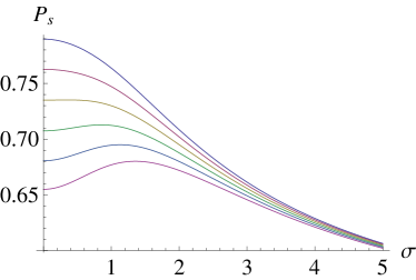
Figure 1: The probability of success $P_{s}$, equation (14), (corresponding to the choice $\wp=1/2$) versus $\sigma$, for the noise-assisted threshold detection. The values of the parameters are $\eta=0.8$, $\alpha_{q}=1$ and $r=0$, giving $\theta_{\pm}\approx\pm 0.96$ after applying Proposition 1. Curves from top to bottom correspond respectively to $\theta=0.85$, $0.95$ (inside the forbidden interval), $1.05$, $1.15$, $1.25$, $1.35$ (outside the forbidden interval). Due to symmetry, we also have the same plot for the values $\theta=-0.85$, $-0.95$, $-1.05$, $-1.15$, $-1.25$, $-1.35$.

Figure 2 plots the forbidden interval in the $\theta,r$ plane. We can see that increasing the squeezing level reduces the width of the forbidden interval up to $2\sqrt{\eta}\,\alpha_{q}$. Similarly, figure 3 plots the forbidden interval in the $\theta,\alpha_{q}$ plane. Increasing the amplitude enlarges the width of the forbidden interval up to $2\sqrt{\eta}\,\alpha_{q}$.

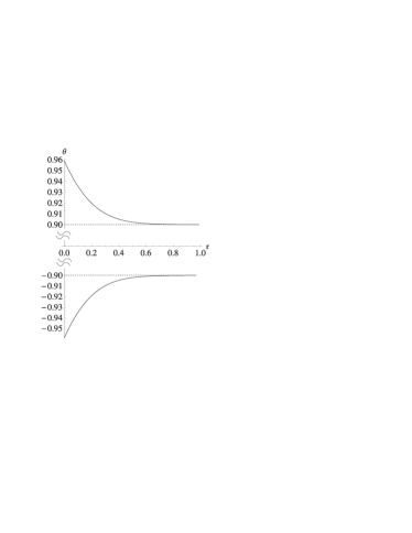
Figure 2: Forbidden interval (area between upper and lower curves) in the $\theta,r$ plane, drawn according to Proposition 1. The top (resp. bottom) solid line corresponds to $\theta_{+}$ (resp. $\theta_{-}$) while the top (resp. bottom) dashed line corresponds to $\sqrt{\eta}\,\alpha_{q}$ (resp. $-\sqrt{\eta}\,\alpha_{q}$). The values of the other parameters are $\wp=1/2$, $\eta=0.8$, and $\alpha_{q}=1$.

Figure 3: Forbidden interval (area between upper and lower curves) in the $\theta,\alpha_{q}$ plane, drawn according to Proposition 1. The top (resp. bottom) solid line corresponds to $\theta_{+}$ (resp. $\theta_{-}$), while the top (resp. bottom) dashed line corresponds to $\sqrt{\eta}\,\alpha_{q}$ (resp. $-\sqrt{\eta}\,\alpha_{q}$). The values of the other parameters are $\wp=1/2$, $\eta=0.8$, and $r=0$.

Finally, notice that Proposition 1 holds true even if the noise $\nu_{q}$ is introduced at the sender’s end.

3 Stochastic Resonance in Entanglement-Assisted Classical Communication

Let us consider the same channel as in the previous section, but we now assume that the sender and receiver share an entangled state, namely, a two-mode squeezed vacuum [16], before communication begins. This situation is somehow similar to the communication scenario in super-dense coding [20], with the exception that we have continuous variable systems and thresholding at the receiver. Let mode 1 (resp. 2) belong to the sender (resp. receiver). The sender displaces her share of the entanglement by the complex number $-\alpha_{q}\left(-1\right)^{X_{q}}-i\alpha_{p}\left(-1\right)^{X_{p}}$ in order to transmit the two bits $X_{q}$ and $X_{p}$. The resulting displaced squeezed vacuum operators are as follows:

$$(\hat{q}_{1}-\hat{q}_{2})e^{-r}-\alpha_{q}(-1)^{X_{q}}\,,$$ (18)

$$(\hat{p}_{1}+\hat{p}_{2})e^{-r}-\alpha_{p}(-1)^{X_{p}}\,,$$ (19)

where $\hat{q}$, $\hat{p}$ are the position, momentum quadrature operators, $r\geqslant 0$ is the squeezing strength, $\alpha_{q},\alpha_{p}\in\mathbbm{R}$ are the displacement amplitudes, and $X_{q},X_{p}\in\{0,1\}$ are binary random variables.

Since $\hat{q}_{1}-\hat{q}_{2}$ commutes with $\hat{p}_{1}+\hat{p}_{2}$, it suffices to analyze the output for (18). After the sender transmits her share of the entanglement through a lossy bosonic channel with transmissivity $\eta\in\left(0,1\right)$, the operator describing their state is as follows:

$$\left(\sqrt{\eta}\,\hat{q_{1}}-\hat{q}_{2}\right)e^{-r}-\sqrt{\eta}\,\alpha_{q}(-1)^{X_{q}}+\sqrt{1-\eta}\,\hat{q}_{E}\,,$$

where $\hat{q}_{E}$ is the position quadrature operator of the environment mode (assumed to be in the vacuum state for the sake of simplicity).

At the receiver’s end, let us again consider the possibility of adding a random, Gaussian-distributed displacement $\nu_{q}\in\mathbbm{R}$ to the arriving state. Then the output observable becomes as follows:

$$\left(\sqrt{\eta}\,\hat{q_{1}}-\hat{q}_{2}\right)e^{-r}-\sqrt{\eta}\,\alpha_{q}(-1)^{X_{q}}+\sqrt{1-\eta}\,\hat{q}_{E}+\nu_{q}\,.$$

Repeating the steps of Section 2, we have

$$S_{X_{q}}=N-\sqrt{\eta}\,\alpha_{q}(-1)^{X_{q}}\,,$$

where now

$$N\equiv\left(\sqrt{\eta}\,\hat{q_{1}}-\hat{q}_{2}\right)e^{-r}+\sqrt{1-\eta}\,\hat{q}_{E}+\nu_{q}\,.$$ (20)

and

$$P_{N}={\mathcal{N}}(0,\eta e^{-2r}/2)\circ{\mathcal{N}}(0,e^{-2r}/2)\circ{\mathcal{N}}(\left(1-\eta\right)/2)\circ{\mathcal{N}}(0,\sigma^{2}_{q}/2)\,,$$ (21)

so that

$$P_{N}=\mathcal{N}\left(0,(1-\eta+(1+\eta)e^{-2r}+\sigma^{2}_{q})/2\right)\,.$$ (22)

The receiver then thresholds the measurement result with a threshold $\theta_{q}\in\mathbbm{R}$, and he retrieves a random bit $Y_{q}$ where

$$Y_{q}\equiv H\left(N-\sqrt{\eta}\,\alpha_{q}(-1)^{X_{q}}-\theta_{q}\right)\,,$$ (23)

and $H$ is the unit Heaviside step function.

Proceeding as in Section 2, we obtain the following input/output conditional probabilities

$$P_{Y_{q}|X_{q}}(0|0) = \frac{1}{2}+\frac{1}{2}\mathrm{erf}\left[\frac{\theta_{q}+\sqrt{\eta}\,\alpha_{q}}{\sqrt{1-\eta+(1+\eta)e^{-2r}+\sigma^{2}_{q}}}\right]\,,$$ (24)

$$P_{Y_{q}|X_{q}}(1|1) = \frac{1}{2}-\frac{1}{2}\mathrm{erf}\left[\frac{\theta_{q}-\sqrt{\eta}\,\alpha_{q}}{\sqrt{1-\eta+(1+\eta)e^{-2r}+\sigma^{2}_{q}}}\right]\,.$$ (25)

Then, writing $P_{X_{q}}(0)=\wp_{q}$ and $P_{X_{q}}(1)=1-\wp_{q}$, the probability of success reads

$${P}_{s,q} = \frac{1}{2}+\frac{1}{2}\wp_{q}\,\mathrm{erf}\left(\frac{\theta_{q}+\sqrt{\eta}\,\alpha_{q}}{\sqrt{1-\eta+(1+\eta)e^{-2r}+\sigma^{2}_{q}}}\right)$$ (26)

$$-\frac{1}{2}(1-\wp_{q})\,\mathrm{erf}\left(\frac{\theta_{q}-\sqrt{\eta}\,\alpha_{q}}{\sqrt{1-\eta+(1+\eta)e^{-2r}+\sigma^{2}_{q}}}\right)\,.$$

Analogously, for the quadrature $\hat{p}_{1}+\hat{p}_{2}$, we have

$${P}_{s,p} = \frac{1}{2}+\frac{1}{2}\wp_{p}\,\mathrm{erf}\left(\frac{\theta_{p}+\sqrt{\eta}\,\alpha_{p}}{\sqrt{1-\eta+(1+\eta)e^{-2r}+\sigma^{2}_{p}}}\right)$$ (27)

$$-\frac{1}{2}(1-\wp_{p})\,\mathrm{erf}\left(\frac{\theta_{p}-\sqrt{\eta}\,\alpha_{p}}{\sqrt{1-\eta+(1+\eta)e^{-2r}+\sigma^{2}_{p}}}\right)\,.$$

We have assumed that the noise terms added to the quadratures $\hat{q}_{1}-\hat{q}_{2}$ and $\hat{p}_{1}+\hat{p}_{2}$ have variances $\sigma_{q}^{2}/2$ and $\sigma_{p}^{2}/2$ respectively.

We finally arrive at the following proposition:

Proposition 2 (The forbidden rectangle)

The probability of success $P_{s}=P_{s,q}P_{s,p}$ shows a non-monotonic behavior vs $\sigma_{q}$, $\sigma_{p}$ iff $\theta_{q}\notin[\theta_{q-},\theta_{q+}]$ or $\theta_{p}\notin[\theta_{p-},\theta_{p+}]$ where $\theta_{\bullet\pm}$ are the roots of the following equation:

$$\frac{\wp_{\bullet}(\theta_{\bullet}+\sqrt{\eta}\,\alpha_{\bullet})}{(1-\wp_{\bullet})(\theta_{\bullet}-\sqrt{\eta}\,\alpha_{\bullet})}=\exp\left[\frac{4\sqrt{\eta}\,\alpha_{\bullet}\theta_{\bullet}}{1-\eta+(1+\eta)e^{-2r}}\right],$$

with $\theta_{\bullet-}\leq-\sqrt{\eta}\,\alpha_{\bullet}<+\sqrt{\eta}\,\alpha_{\bullet}\leq\theta_{\bullet+}$ (here $\bullet$ stands for either $q$ or $p$).

Proof. The proof can be obtained from that of Proposition 1 after replacing $-\eta+\eta e^{-2r}$ with $-\eta+(1+\eta)e^{-2r}$.   

It is worth remarking in the above proposition that either of the conditions $\theta_{q}\notin[\theta_{q-},\theta_{q+}]$ or $\theta_{p}\notin[\theta_{p-},\theta_{p+}]$ (or both) have to be satisfied in order to have a non monotonic behavior for $P_{s}$. This follows because $P_{s}$ is a function of two variables $\sigma_{q}^{2}$ and $\sigma_{p}^{2}$, hence it suffices that the partial derivative with respect to one of them has a maximum to have a non-monotonic behavior. As consequence we have a “forbidden rectangle” rather than “forbidden stripes” in the $\theta_{q},\theta_{p}$ plane.

It is also worth noticing the difference of the equation in the above proposition with that in the proposition of the previous section. Here the squeezing factor $e^{-2r}$ is multiplied by $(1+\eta)$ rather than $\eta$. This is because we now have two squeezed modes, one of which is attenuated by the lossy channel.

Finally, notice that Proposition 2 holds true even if the noise $\nu_{q}$ is introduced at the sender’s end.

4 Stochastic Resonance in Channel Discrimination

Let us now consider two lossy quantum channels with transmissivities $\eta_{0},\eta_{1}\in(0,1)$ (suppose, without loss of generality, $\eta_{0}>\eta_{1}$). Our aim is to distinguish them. Differently from previous works, here we do not optimize over all possible decoding strategies [21], but concentrate on a given threshold-detection scheme. Then, suppose to use as probe (input) a squeezed and displaced vacuum operator

$$\hat{q}e^{-r}+\alpha_{q}\,,$$ (28)

where $\hat{q}$ is the position quadrature operator, $r$ is the squeezing parameter, and $\alpha_{q}\in\mathbbm{R}$ the displacement amplitude.

The transmission through the lossy channel with transmissivity $\eta_{X}$, $X=0,1$, can be considered as the encoding of a binary random variable $X=0,1$ occurring with probability $P_{X}$. The output observable after transmission is then

$$\sqrt{\eta_{X}}\left(\alpha_{q}+\hat{q}e^{-r}\right)+\sqrt{1-\eta_{X}}\,\hat{q}_{E}\,,$$

where $\hat{q}_{E}$ is the position quadrature operator of the environment mode (assumed to be in the vacuum state for the sake of simplicity).

At the receiver’s end, we consider the addition of noise, modeled by a random, Gaussian-distributed displacement $\nu_{q}\in\mathbbm{R}$. Then the output observable becomes

$$\sqrt{\eta_{X}}\left(\alpha_{q}+\hat{q}e^{-r}\right)+\sqrt{1-\eta_{X}}\,\hat{q}_{E}+\nu_{q}\,.$$

Upon measurement of the position quadrature operator, the signal value is

$$S_{X}=\sqrt{\eta_{X}}\left(\alpha_{q}+qe^{-r}\right)+\sqrt{1-\eta_{X}}\,q_{E}+\nu_{q}\,.$$ (29)

We define a conditional random variable $N|X$ summing all noise terms:

$$N|X\equiv\sqrt{\eta_{X}}\,qe^{-r}+\sqrt{1-\eta_{X}}\,q_{E}+\nu_{q}\,.$$ (30)

The density $P_{N|X}\left(n|x\right)$ of the random variable $N|X$ is

$$P_{N|X}={\mathcal{N}}(0,\eta_{x}e^{-2r}/2)\circ{\mathcal{N}}(0,\left(1-\eta_{x}\right)/2)\circ{\mathcal{N}}(0,\sigma^{2}/2)\,.$$ (31)

Notice that the noise term (30) explicitly depends on the encoded value $X$ and so does its probability density. From (31), we explicitly obtain

$$P_{N|X}=\mathcal{N}\left(0,(1-\eta_{x}+\eta_{x}e^{-2r}+\sigma^{2})/2\right)\,.$$ (32)

The output signal (29) can now be written as

$$S_{X}=\sqrt{\eta_{X}}\,\alpha_{q}+N|X\,.$$

The receiver then thresholds the measurement result with a threshold $\theta\in\mathbbm{R}$ to retrieve a random bit $Y$ where

$$Y\equiv H\left(\theta-\sqrt{\eta_{X}}\,\alpha_{q}-N|X\right)\,,$$

and $H$ is the unit Heaviside step function. In this case, the receiver assigns $Y=1$ if the output signal $S_{X}$ is smaller that the threshold, and assigns $Y=0$ otherwise.

The final detected bit $Y$ should be the same as the encoded bit $X$. Hence, the probability of success reads like (13) where now

$$P_{Y|X}(0|0) = \int_{-\infty}^{+\infty}\left[1-H\left(\theta-\sqrt{\eta_{0}}\,\alpha_{q}-n\right)\right]P_{N|X}\left(n|0\right)dn\,,$$

$$P_{Y|X}(1|1) = \int_{-\infty}^{+\infty}H\left(\theta-\sqrt{\eta_{1}}\,\alpha_{q}-n\right)P_{N|X}\left(n|1\right)dn\,.$$

Using (32) we obtain

$$P_{Y|X}(0|0) = \frac{1}{2}\left[1-\mathrm{erf}\left(\frac{\theta-\sqrt{\eta_{0}}\,\alpha_{q}}{\sqrt{1-\eta_{0}+\eta_{0}e^{-2r}+\sigma^{2}}}\right)\right]\,,$$ (33)

$$P_{Y|X}(1|1) = \frac{1}{2}\left[1+\mathrm{erf}\left(\frac{\theta-\sqrt{\eta_{1}}\,\alpha_{q}}{\sqrt{1-\eta_{1}+\eta_{1}e^{-2r}+\sigma^{2}}}\right)\right]\,.$$ (34)

Then, writing $P_{X}\left(0\right)=\wp$ and $P_{X}\left(1\right)=1-\wp$, we get

$${P}_{s} = \frac{1}{2}-\frac{1}{2}\wp\,\mathrm{erf}\left(\frac{\theta-\sqrt{\eta_{0}}\,\alpha_{q}}{\sqrt{1-\eta_{0}+\eta_{0}e^{-2r}+\sigma^{2}}}\right)$$ (35)

$$+\frac{1}{2}(1-\wp)\,\mathrm{erf}\left(\frac{\theta-\sqrt{\eta_{1}}\,\alpha_{q}}{\sqrt{1-\eta_{1}+\eta_{1}e^{-2r}+\sigma^{2}}}\right)\,.$$

Our aim is to analyze the probability of success as a function of the noise variance, for given values of the parameters $\alpha_{q}$, $r$, $\theta$, $\eta_{0}$, $\eta_{1}$.

In the simplest case of $r=0$, we have the following proposition:

Proposition 3 (The forbidden interval)

The probability of success $P_{s}$ shows a non-monotonic behavior as a function of $\sigma$ iff $\theta\notin[\theta_{-},\theta_{+}]$, where $\theta_{\pm}$ are the two roots of the following equation:

$$\frac{\wp(\theta-\sqrt{\eta_{0}}\,\alpha_{q})}{(1-\wp)(\theta-\sqrt{\eta_{1}}\,\alpha_{q})}=\exp\left[\alpha_{q}^{2}(\eta_{0}-\eta_{1})-2\alpha_{q}\theta(\sqrt{\eta_{0}}-\sqrt{\eta_{1}})\right]\,,$$ (36)

such that $\theta_{-}\leqslant\sqrt{\eta_{1}}\,\alpha_{q}<\sqrt{\eta_{0}}\,\alpha_{q}\leqslant\theta_{+}$.

Proof. We consider the probability of success as a function of $\sigma^{2}$. In order to have a non-monotonic behavior for ${P}_{s}(\sigma^{2})$, we must check for the presence of a local maximum. By solving

$$\frac{d{P}_{s}(\sigma^{2})}{d\sigma^{2}}=0\,,$$ (37)

we obtain the following expression for the critical value of $\sigma^{2}$:

$$\sigma_{\ast}^{2}=-1+\frac{\alpha_{q}^{2}(\eta_{0}-\eta_{1})-2\alpha_{q}\theta(\sqrt{\eta_{0}}-\sqrt{\eta_{1}})}{\ln\left[\frac{\wp(\theta-\sqrt{\eta_{0}}\,\alpha_{q})}{(1-\wp)(\theta-\sqrt{\eta_{1}}\,\alpha_{q})}\right]}\,.$$ (38)

The condition for non-monotonicity of the probability of success as a function of $\sigma^{2}$, $\sigma_{\ast}^{2}>0$, is verified iff $\theta\not\in[\theta_{-},\theta_{+}]$, where $\theta_{\pm}$ are the roots of $\sigma_{\ast}^{2}=0$, i.e., equation (36). Finally, equation (36) implies $\frac{\theta-\sqrt{\eta_{0}}\,\alpha_{q}}{\theta-\sqrt{\eta_{1}}\,\alpha_{q}}>0$, which in turn yields $\theta_{-}\leqslant\sqrt{\eta_{1}}\,\alpha_{q}<\sqrt{\eta_{0}}\,\alpha_{q}\leqslant\theta_{+}$.   

If $r\neq 0$, (37) is not algebraic—hence we did not succeed in providing an analytical expression for $\sigma_{\ast}^{2}$. However, numerical investigations show a qualitative behavior of the forbidden interval’s boundaries identical to that shown in figures 2 and 3 (notice that here $-\sqrt{\eta}\,\alpha_{q}$ and $\sqrt{\eta}\,\alpha_{q}$ are replaced by $\sqrt{\eta_{1}}\,\alpha_{q}$ and $\sqrt{\eta_{0}}\,\alpha_{q}$, respectively).

Finally, notice that Proposition 3 holds true even if the noise $\nu_{q}$ is introduced at the sender’s end.

5 Stochastic Resonance in Quantum Communication

Let us now consider a setting in which the SR effect can occur in the transmission of a qubit ($Q$). The aim is to first encode a qubit state into a bosonic mode ($B$) state, send it through the lossy channel, and finally coherently decode, with a threshold mechanism, the output bosonic mode state into a qubit system at the receiving end. We should qualify that it is unclear to us whether one would actually exploit the encodings and decodings given in this section, but regardless, the setting given here provides a novel scenario in which the SR effect can occur for a quantum system. We might consider the development in this section to be a coherent version of the settings in the previous sections. Also, it is in the spirit of a true “quantum stochastic resonance” effect hinted at in Ref. [22].

We work in the Schrödinger picture, and consider an initial state $|\varphi\rangle_{Q}\otimes|0\rangle_{B}$, where $|\varphi\rangle_{Q}=a|0\rangle_{Q}+b|1\rangle_{Q}$ is an arbitrary qubit state and $|0\rangle_{B}$ is the zero-eigenstate of the position-quadrature operator of the bosonic field. Here for the sake of simplicity we are going to work with infinite-energy position eigenstates rather than with squeezed-coherent states.

Suppose that the encoding takes place through the following unitary controlled-operations:

$$U_{1}^{QB} = \left|0\right\rangle_{Q}\left\langle 0\right|\otimes e^{-i\hat{p}_{B}x_{0}}+\left|1\right\rangle_{Q}\left\langle 1\right|\otimes e^{i\hat{p}_{B}x_{0}}\,,$$ (39)

$$U_{2}^{QB} = I_{Q}\otimes\int_{x\geqslant 0}\left|x\right\rangle_{B}\left\langle x\right|dx+X_{Q}\otimes\int_{x<0}\left|x\right\rangle_{B}\left\langle x\right|dx\,,$$ (40)

where $I_{Q}=|0\rangle_{Q}\langle 0|+|1\rangle_{Q}\langle 1|$ and $X_{Q}=|0\rangle_{Q}\langle 1|+|1\rangle_{Q}\langle 0|$, $\hat{p}_{B}$ denotes the canonical momentum operator of the bosonic system, $|\pm x_{0}\rangle$ are the generalized eigenstates of the canonical position operator $\hat{q}_{B}$, and we assume, without loss of generality, $x_{0}\in\mathbbm{R}_{+}$. This encoding is a coherent version of encoding a binary number into an analog signal.

The effect of such operations on the initial states is

$$U_{2}^{QB}U_{1}^{QB}|\varphi\rangle_{Q}\otimes|0\rangle_{B}=|0\rangle_{Q}\otimes\left(a|x_{0}\rangle_{B}+b|-x_{0}\rangle_{B}\right).$$ (41)

Now, with the bosonic mode state factored out from the qubit state, it can be sent through the lossy channel. For the sake of analytical investigation, we consider a channel with unit trasmittivity (an identity channel). Then, the output state simply reads

$$\rho_{B}=\left(a|x_{0}\rangle+b|-x_{0}\rangle\right)_{B}\left(\overline{a}\,\langle x_{0}|+\overline{b}\,\langle-x_{0}|\right),$$

At this point we consider the possibility of adding Gaussian noise before the (threshold) decoding stage. This is modeled as a Gaussian-modulated displacement of the quadrature $\hat{q}_{B}$. The resulting state will be

$$\rho_{B^{\prime}}=\int dq\,\,{\mathcal{N}}(0,\sigma^{2})D(q,0)\rho_{B}D^{{\dagger}}(q,0)\,,$$ (42)

where $D(q,0)$ is the displacement operator (displacing only in the $\hat{q}_{B}$ direction), and ${\mathcal{N}}(0,\sigma^{2})$ is a zero-mean, Gaussian distribution with variance $\sigma^{2}$.

Now, the state $\rho_{B^{\prime}}$ is decoded into a qubit system $Q^{\prime}$ initially prepared in the state $|0\rangle_{Q^{\prime}}$ through the following controlled-unitary operations involving a coherent threshold mechanism

$$V_{1}^{Q^{\prime}B^{\prime}} = I_{Q}\otimes\int_{x\geqslant\theta}\left|x\right\rangle_{B}\left\langle x\right|dx+X_{Q}\otimes\int_{x<\theta}\left|x\right\rangle_{B}\left\langle x\right|dx\,,$$ (43)

$$V_{2}^{Q^{\prime}B^{\prime}} = \left|0\right\rangle_{Q}\left\langle 0\right|\otimes e^{i\hat{p}_{B}x_{0}}+\left|1\right\rangle_{Q}\left\langle 1\right|\otimes e^{-i\hat{p}_{B}x_{0}}\,.$$ (44)

Clearly, if $\theta=0$ the decoding unitaries (43), (44) are the inverse of the encoding ones (39), (40). They hence allow unit fidelity encoding/decoding if $\sigma^{2}=0$. However, if $\theta\neq 0$, there could be a nonzero optimal value of $\sigma^{2}$.

The final qubit state is

$$\rho_{Q^{\prime}} = \mathcal{E}(|\varphi\rangle_{Q}\langle\varphi|)$$ (45)

$$= {\rm Tr}_{B^{\prime}}\left\{V_{2}^{Q^{\prime}B^{\prime}}V_{1}^{Q^{\prime}B^{\prime}}\left(|0\rangle_{Q}^{\prime}\langle 0|\otimes\rho_{B^{\prime}}\right)\left(V_{1}^{Q^{\prime}B^{\prime}}\right)^{{\dagger}}\left(V_{2}^{Q^{\prime}B^{\prime}}\right)^{{\dagger}}\right\}$$ (47)

$$= \left[|a|^{2}(1-\Pi_{<})+|b|^{2}\Pi_{>})\right]|0\rangle_{Q}\langle 0|+\left[|a|^{2}\Pi_{<}+|b|^{2}(1-\Pi_{>})\right]|1\rangle_{Q}\langle 1|$$

$$+(1-\Pi_{<}-\Pi_{>})\left(a\bar{b}|0\rangle_{Q}\langle 1|+\bar{a}b|1\rangle_{Q}\langle 0|\right)\,,$$

where

$$\Pi_{<} = \frac{1}{2}+\frac{1}{2}{\rm erf}\left(\frac{\theta-x_{0}}{\sqrt{2\sigma^{2}}}\right)\,,$$ (48)

$$\Pi_{>} = \frac{1}{2}-\frac{1}{2}{\rm erf}\left(\frac{\theta+x_{0}}{\sqrt{2\sigma^{2}}}\right)\,.$$ (49)

Then we can calculate the average channel fidelity

$$\langle\mathcal{F}\rangle=\int d\varphi\,\,{}_{Q}\langle\varphi|\rho_{Q^{\prime}}|\varphi\rangle_{Q}\,,$$ (50)

where $d\varphi$ is the uniform measure induced by the Haar measure on $\mathrm{SU}(2)$.

Using (42), (43), (44), (45) and (50) we finally obtain

$$\langle\mathcal{F}\rangle=\frac{1}{2}+\frac{1}{4}\left[{\rm erf}\left(\frac{\theta+x_{0}}{\sqrt{2\sigma^{2}}}\right)-{\rm erf}\left(\frac{\theta-x_{0}}{\sqrt{2\sigma^{2}}}\right)\right].$$ (51)

Then, we have the following proposition:

Proposition 4

[The forbidden interval] The average channel fidelity $\langle\mathcal{F}\rangle$ shows a non-monotonic behavior as a function of $\sigma$ iff $\theta\notin[-x_{0},x_{0}]$.

Proof. We consider $\langle\mathcal{F}\rangle$ as a function of $\sigma^{2}$. In order to have a non-monotonic behavior, we must check for the presence of a local maximum for $\sigma^{2}>0$. The condition $\frac{d\langle F\rangle}{d\sigma}=0$ yields the following expression for the critical value of $\sigma^{2}$

$$\sigma^{2}_{\ast}=\frac{2\theta x_{0}}{\ln\left(\frac{\theta+x_{0}}{\theta-x_{0}}\right)}\,.$$ (52)

We hence conclude that the average fidelity is a non-monotonic function of $\sigma$ iff $\theta\notin[-x_{0},x_{0}]$.   

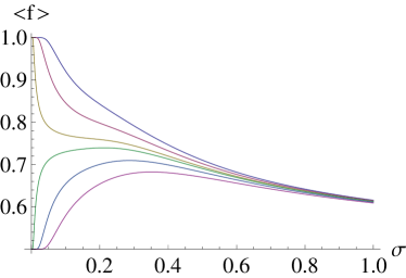
Figure 4: The average channel fidelity $\langle\mathcal{F}\rangle$, equation (51) vs $\sigma$ for $x_{0}=0.3$ and several values of $\theta$, inside and outside the forbidden interval. From top to bottom, $\theta=0.20$, $\theta=0.25$, $\theta=0.29$ (inside the forbidden interval), $\theta=0.31$, $\theta=0.35$, $\theta=0.40$ (outside the forbidden interval).

Figure 4 shows $\langle\mathcal{F}\rangle$ as a function of $\sigma$ for a given value of $x_{0}$ and several values of $\theta$, both inside and outside the forbidden interval. A non-monotonic behavior is observed in the latter cases. It is worth noticing that the presence of noise can augment the average channel fidelity above the value of $2/3$, which is the maximum value achievable by measure-and-prepare protocols. Hence, in this sense, the presence of noise can lead to a transition from a classical to a quantum regime in the average communication fidelity.

As shown in figure 5, an analogous SR-like effect is observed in the same parametric region for the logarithmic negativity [23]

$$LN=\log_{2}\left\{\mathrm{Tr}\left[\mathcal{E}\otimes\mathcal{I}\left(|\Psi\rangle\langle\Psi|\right)\right]^{\Gamma}\right\}\,,$$ (53)

where $\Gamma$ indicates the partial transpose operation, $\mathcal{I}$ the identity map and $|\Psi\rangle$ a maximally entangled two-qubit Bell state. This quantity is the logarithmic negativity of the Choi-Jamiolkowski state associated to the quantum channel [24] and gives an upper bound on its two-way distillable entanglement (this latter quantity in turn equals the quantum capacity of a channel assisted by unbounded two-way classical communication [25]).

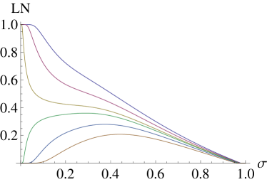
Figure 5: The logarithmic negativity, equation (53), vs $\sigma$ for $x_{0}=0.3$ and several values of $\theta$ inside and outside the forbidden interval. From top to bottom, $\theta=0.20$, $\theta=0.25$, $\theta=0.29$ (inside the forbidden interval), $\theta=0.31$, $\theta=0.35$, $\theta=0.40$ (outside the forbidden interval).

Finally, notice that Proposition 4 holds true even if the noise $\nu_{q}$ is introduced at the sender’s end.

6 Stochastic Resonance in Quantum Key Distribution

In this section we investigate stochastic resonance effects in quantum key distribution (see also [6, 9]). An achievable rate for private classical communication over a quantum channel is given by the following formula [26, 27]:

$$C_{P}=I(A:B)-I(A:E)\,,$$ (54)

where $I(A:B)$ and $I(A:E)$ are the maximal mutual information between sender ($A$) and receiver ($B$) and sender and eavesdropper ($E$), respectively. In the above formula, $A$ is a classical system, $B$ and $E$ are quantum systems, and the optimization is over all ensembles that Alice can prepare at the input.

We consider the same encoding of a binary variable into a single bosonic mode expressed by Eq. (1). Also, we consider the case in which information is transmitted through a lossy bosonic channel characterized by the transmissivity parameter $\eta$ [15]. The input variable after the transmission through the noisy channel is hence expressed by Eq. (2).

First, suppose that the noise is added at the receiver’s end. In this case, the quantity $I(A:E)$ is not affected at all by the noise, and so the behavior of $C_{P}$ versus $\sigma$ is simply determined by $I(A:B)$. Since this latter relies on the probability of success given by equation (14), we are in the same situation as in Proposition 1. In particular, the private communication rate in Eq. (54) exhibits a non-monotonic behavior as a function of the noise variance if and only if the threshold value $\theta$ lies outside of the forbidden interval $[\theta_{-},\theta_{+}]$, where $\theta_{\pm}$ are the two roots of equation (15).

Second, suppose that the noise is added at the sender’s end. In this case, equation (3) changes as follows:

$$\sqrt{\eta}\left(\hat{q}e^{-r}-\alpha_{q}(-1)^{X}+\nu_{q}\right)+\sqrt{1-\eta}\,\hat{q}_{E}\,.$$ (55)

Using a threshold decoding, we get the same expression as in equation (14) for the success probability, upon replacing $\sigma^{2}\to\eta\sigma^{2}$. From this, it is straightforward to calculate the mutual information $I(A:B)$. In turn, we assume that the eavesdropper has access to the conjugate mode at the output of the beam-splitter transformation, and so its variable is given by

$$\sqrt{1-\eta}\left(\hat{q}e^{-r}-\alpha_{q}(-1)^{X}+\nu_{q}\right)+\sqrt{\eta}\,\hat{q}_{E}\,.$$ (56)

The maximum mutual information between the sender and eavesdropper is given in terms of the Holevo information [28]. Since the average state corresponding to the variable (56) is non-Gaussian, the analytical evaluation of its Holevo information appears not to be possible. However, the monotonicity property of the Holevo information under composition of quantum channels ensures that it has to be a monotonically decreasing function of the noise variance $\sigma^{2}/2$. As a consequence, we expect that its contribution to the private communication rate will increase with increasing value of the noise. Indeed, a numerical analysis suggests that the private communication rate can exhibit a non-monotonic behavior as function of $\sigma$ for all values of $\theta$. Examples of this behavior are shown in figure 6.

We are then led to formulate the following conjecture:

Conjecture 5

[The forbidden interval] The private communication rate $C_{P}$ shows a non-monotonic behavior as a function of $\sigma$ for all $\theta\in\mathbbm{R}$ if $\nu_{q}$ is added at the sender’s end.

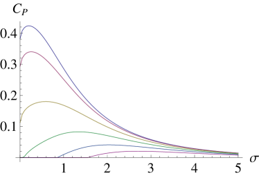
Figure 6: The private communication rate (corresponding to the choice $\wp=1/2$), equation (54), versus $\sigma$, for the case of noise added by the sender. The values of the parameters are $\eta=0.8$, $\alpha_{q}=1$ and $r=0$. Curves from top to bottom correspond respectively to $\theta=0$, $0.5$, $1$, $1.5$, $2$, $2.5$.

7 Conclusion

In conclusion, we have determined necessary and sufficient conditions for observing SR when transmitting classical, private, and quantum information over a lossy bosonic channel or when discriminating lossy channels. Nonlinear coding and decoding by threshold mechanisms have been exploited together with the addition of Gaussian noise.

Specifically, we have considered a bit encoded into coherent states with different amplitudes that are subsequently sent through a lossy bosonic channel and decoded at the output by threshold measurement of their amplitudes (without and with the assistance of entanglement shared by sender and receiver). We have also considered discrimination of lossy bosonic channels with different loss parameters. In all these cases, the performance is evaluated in terms of success probability. Since the mutual information is a monotonic function of this probability, the same conclusions can be drawn in terms of mutual information.

SR effects appear whenever the threshold lies outside of the different forbidden intervals that we have established. If it lies inside of a forbidden interval, then the SR effect does not occur. Actually, absolute maxima of success probability are obtained when the threshold is set in the middle of the forbidden interval.

Generally speaking, SR effects are known to improve analog-to-digital conversion performance [29]. In fact, if two distinct signals by continuous-to-binary conversion fall within the same interval they can no longer be distinguished. In such a situation the addition of a moderate amount of noise turns out to be useful as long as it shifts the signals apart to help in distinguishing them. While it is important to confirm this possibility also in the quantum framework, we have also shown that the same kind of effects may arise in a purely quantum framework. Indeed, we have also considered the transmission of quantum information, represented by a qubit which is encoded into the state of a bosonic mode and then decoded according to a threshold mechanism. The found nonmonotonicity of the average channel fidelity and of the output entanglement (quantified by the logarithmic negativity) outside the forbidden interval, represents a clear signature of a purely quantum SR effect.

In all the above mentioned cases it does not matter whether the sender or the receiver adds the noise. The exception occurs when the goal is to transmit private information. In fact, by considering achievable rates for private transmission over the lossy channel, we have pointed out that the forbidden interval can change drastically, depending on whether the receiver or the sender adds noise. In the former case, it is exactly the same as the case of sending classical (non private) information. In the latter case, we conjecture that it vanishes, i.e., the noise addition turns out to be beneficial always. This feature of the private communication rate can be interpreted as a consequence of the asymmetry between the legitimate receiver of the private information and the eavesdropper. In fact, while the legitimate receiver is restricted to threshold detection, we have allowed the eavesdropper to use more general detection schemes.

References

References

- [1] Gammaitoni L, Hänggi P, Jung P and Marchesoni F 1998 Rev. Mod. Phys. 70 223
- [2] Kosko B 2006 Noise (London, Viking Penguin)
- [3] Patel A and Kosko B 2009 IEEE Trans. Signal Proc., 57, 1655
- [4] Ting J. J.-L. 1999 Phys. Rev. E 59 2801
-
[5]
Bowen G and Mancini S 2004 Phys. Lett. A 321 1
Bowen G and Mancini S 2006 Phys. Lett. A 352 272 - [6] Renner R, Gisin N and Kraus B 2005 Phys. Rev. A 72 012332
- [7] Wilde M M 2009 J. Phys. A 42 325301
- [8] Wilde M M and Kosko B 2009 J. Phys. A 42 465309
-
[9]
Pirandola S, García-Patrón R, Braunstein S L and Lloyd S 2009
Phys. Rev. Lett. 102 050503
García-Patrón R and Cerf N. J. 2009 Phys. Rev. Lett. 102 130501 - [10] Caruso F, Huelga S F and Plenio M B 2010 Phys. Rev. Lett. 105 190501
-
[11]
Stein S and Jay Jones J 1967
Modern communication principles,
(New York, McGraw Hill)
Gray R M and Neuhoff D L 1998 IEEE Trans. Inf. Th. 44 2325 - [12] Kosko B and Mitaim S 2003 Neural Networks 16 755
- [13] Wiseman H M and Milburn G. J. 1993 Phys. Rev. A 47 642
- [14] Eisert J and Wolf M M 2007 in Quantum Information with Continuous Variables, edited by N. J. Cerf, G. Leuchs, and E. Polzik (London, Imperial College Press)
- [15] Holevo A S and Werner R F 2001 Phys. Rev. A 63 032312
- [16] Gerry C C and Knight P L 2005 Introductory Quantum Optics (Cambridge, Cambridge University Press)
- [17] Rousseau D, Anand G V and Chapeau-Blondeau F 2006 Signal Processing 86 3456
- [18] Patel A and Kosko B 2009 Neural Networks 22 697
- [19] Mitaim S and Kosko B 1998 Proceedings of the IEEE 86 2152
-
[20]
Bennett C H and Wiesner S J 1992
Phys. Rev. Lett. 69 2881
Braunstein S L and Kimble H J 2000 Phys. Rev. A 61 042302 -
[21]
Pirandola S 2011
Phys. Rev. Lett. 106 090504
Invernizzi C, Paris M G A and Pirandola S 2011 Phys. Rev. A 84 022334 - [22] Bulsara A R 2005 Nature 437 962
- [23] Plenio M B 2005 Phys. Rev. Lett. 95 090503
- [24] Jamiołkowski A 1972 Rep. Math. Phys. 3 275
- [25] Bennett C H, DiVincenzo D P, Smolin J A and Wootters W K 1996 Phys. Rev. A 54 3824
- [26] Devetak I 2005 IEEE Trans. Inf. Th. 51 44
- [27] Cai N, Winter A and Yeung R W 2004 Problems of Information Transmission 40 318
- [28] Holevo A S 1973 Probl. Peredachi Inf. 9 177
- [29] Gammaitoni L 1995 Phys. Rev. E 52 4691