Cumulative compressibility effects on population dynamics in turbulent flows

Abstract

Bacteria and plankton populations living in oceans and lakes reproduce and die under the influence of turbulent currents. Turbulent transport interacts in a complex way with the dynamics of populations because the typical reproduction time of microorganism is within the inertial range of turbulent time scales. In the present manuscript we quantitatively investigate the effect of flow compressibility on the dynamics of populations. While a small compressibility can be induced by several physical mechanisms, like density mismatch or the finite size of microorganisms with respect to the fluid turbulence, its effect on the the carrying capacity of the ecosystem can be dramatic. We report, for the first time, how a small compressibility can produce a sizeable reduction in the carrying capacity, due to an integrated effect made possible by the long replication times of the organisms with respect to turbulent time scales. A full statistical quantification of the fluctuations of population concentration field leads to data collapse over a broad range in parameter space.

Bacterial colonies living on a nutrient-rich hard agar dish are commonly described in terms of the Fisher-Kolmogorov-Petrovsky-Piscounov (FKPP) equation of population dynamics fisher . On a rigid substrate the FKPP equation includes only diffusion and growth terms. In a fluid environment the flow can play an important role by means of the advective transport of microorganisms, both at low Wakika , as well as at high Reynolds numbers. In particular, in oceans and lakes microorganisms have found ways to thrive and prosper in high Reynolds number fluid environments.

As discussed in 1d ; per10 , the advection by means of a compressible turbulent flow can lead to highly non-trivial dynamics. Two striking effects emerge: for small enough growth rate, $\mu$, the population concentration field, $c({\bm{x}},t)$, is strongly localized near the transient but long-living sinks of the turbulent flows; in the same limit, the average space-time concentration of the population (carrying capacity) becomes much smaller than its maximum value in absence of flow. Both effects have important biological implications. Recently it was shown that this phenomenology holds true in the case of more realistic two dimensional compressible turbulent velocity fields per10 .

In this manuscript we present new results that support the key role played by even a slight level of compressibility. We have in mind a simplified model for photosynthetic microorganisms that actively control their buoyancy to maintain themselves at a fixed depth below the surface of a turbulent fluid. Small density mismatches or inertial effects due to the finite size of the microorganisms can also lead to an effectively compressible flow tos09 .

The main result of our investigation is that the overall carrying capacity can be described as a universal function of the non-dimensional growth rate and compressibility. Our results imply that even a small compressibility leads to a substantial reduction in the overall carrying capacity.

Bacterial populations in nutrient rich environments can be modeled in terms of the following Fisher-Kolmogorov-Petrovsky-Piscunov (FKPP) equation:

$${\frac{\partial c}{\partial t}}+{\bm{\nabla}}\cdot({\bm{u}}c)=D\nabla^{2}c+\mu c(1-c).$$ (1)

The above equation describes the evolution of the microorganisms concentration field, $c({\bm{x}},t)$, under the effect of advective transport by means of a (turbulent) velocity field, ${\bm{u}}({\bm{x}},t)$, and in presence of spatial diffusivity with a diffusion constant, $D$, and a replication rate, $\mu$. The parameters $D$ and $\mu$ encode important biological information which may depend on the amount of nutrients, temperature, organismic motility and many other parameters of the ecosystem. In Eq. (1) the averaged population density in absence of flow which can be sustained by the ecosystem has been rescaled to $1$; hence our concentration field $c$ is dimensionless. As an example of “life at high Reynolds number” one could consider the FKPP equation [Eq. (1)] to represent the density of the marine cyanobacteria Synechococcus moo95 under conditions of abundant nutrients (so that $\mu\sim constant$).

$\theta$	$\kappa$	$E$	$\varepsilon$	$\tau_{\eta}$	$Z_{\mu\to 0}$
$0$	$0.0$	$3.17$	$0.61$	$5.80\cdot 10^{-2}$	$1.0$
$15$	$1.45\cdot 10^{-2}$	$3.14$	$0.55$	$6.10\cdot 10^{-2}$	$6.8\cdot 10^{-1}$
$30$	$6.50\cdot 10^{-2}$	$2.76$	$0.47$	$6.60\cdot 10^{-2}$	$3.2\cdot 10^{-1}$
$45$	$1.62\cdot 10^{-1}$	$2.24$	$0.36$	$7.60\cdot 10^{-2}$	$1.6\cdot 10^{-1}$
$60$	$3.90\cdot 10^{-1}$	$1.68$	$0.25$	$8.90\cdot 10^{-2}$	$4.1\cdot 10^{-2}$
$75$	$7.50\cdot 10^{-1}$	$1.38$	$0.15$	$1.16\cdot 10^{-1}$	$8.4\cdot 10^{-3}$
$90$	$1.0$	$1.25$	$0.12$	$1.31\cdot 10^{-1}$	$1.6\cdot 10^{-3}$

Table 1: For different values of $\theta$, the compressibility $\kappa$, the energy $E\equiv\frac{1}{L^{2}}\int u^{2}{\rm d}x{\rm d}y$, the energy dissipation rate $\varepsilon\equiv\frac{\nu}{L^{2}}\int(\nabla{\bm{u}})^{2}{\rm d}x{\rm d}y$, the Kolmogorov time scale $\tau_{\eta}$ used in our simulations. Different values of the compressibility are obtained by projecting out the compressible and incompressible component of our $2d$ compressible field for $\kappa=0.16$ as discussed in the text. The energy and dissipation are rounded off to two decimal places.

In this study we build a simple model of microorganisms living in a localized layer at some depth e.g. under the ocean surface. For this reason we will consider a two-dimensional planar surface, taken out of a fully three dimensional turbulent flow. A projected two dimensional slice from a fully 3d velocity field is compressible. The dimensionless numbers characterizing the evolution of the scalar field, $c({\bm{x}},t)$, are the Schmidt number $Sc=\nu/D$ and the dimensionless growth rate $\mu\tau_{\eta}$. Here $\tau_{\eta}\equiv(\nu/\varepsilon)^{1/2}$ is the Kolmogorov dissipative time scale and $\varepsilon$ is the energy dissipation rate of the fluid. A particularly interesting regime arises when the growth time $\tau_{g}\equiv\mu^{-1}$ lies in the middle of the inertial range. Although many factors can affect the estimates, this is the case for oceanic cyanobacteria and phytoplankton living in an turbulent ocean. Indeed, oceanic turbulence has eddies with turnover times ranging from minutes to months while typical microorganism doubling times range from half an hour to half a day mck09 ; mar03 .

Details of the numerical simulations can be found in per10 . The velocity time series of the two dimensional slice were filtered in order to produce time histories with different degrees of compressibility. By projecting the velocity field into an incompressible, ${\bm{u}}^{i}$, and compressible part, ${\bm{u}}^{c}$, we could define a family of velocity fields ${\bm{u}}\equiv\sqrt{2}[{\bm{u}}^{c}\sin(\theta)+{\bm{u}}^{i}\cos(\theta)]$ with $0\leq\theta\leq\pi/2$. The dimensionless compressibility of each new flow is $\kappa\equiv(\nabla\cdot{\bm{u}})^{2}/(\nabla{\bm{u}})^{2}$. For $\theta=0$ the velocity field is purely incompressible, $\kappa=0$, whereas for $\theta=\pi/2$ it is a potential flow, $\kappa=1$. The case $\theta=\pi/4$ corresponds to the flow studied in per10 . In Table 1 we report the values of the compressibility used. The carrying capacity of the ecosystem is defined as:

$$Z=\langle\frac{1}{L^{2}}\int c({\bf x},t)\rm{d^{2}x}\rangle,$$ (2)

where the integral runs over a square domain of size $L^{2}$ with periodic boundary conditions and $\langle\rangle$ indicates temporal averaging. In Fig. 1 we report $Z$ as a function of the dimensionless growth rate, $\mu\tau_{\eta}$, for different values of the flow compressibility (we recall that in absence of flow $Z=1$). The shaded region on the right represents $\mu\tau_{\eta}>1$, while the left shaded region reflects the condition $\mu\tau_{\eta}<\tau_{\eta}/\tau_{L}$, where $\tau_{L}=L/\sqrt{E}$ is the large eddy turnover time. For large growth rates the curves saturate towards unity, although for smaller compressibility the drop in carrying capacity shifts to smaller and smaller growth rates, $\mu\tau_{\eta}$. Note that even at very small values of the compressibility (e.g. $\kappa=0.0145$) there is a significant reduction of the carrying capacity, $\sim 20\%$, for small growth rates. This regime is particularly relevant to marine biology where compressibility is small but the orgamisms have a very slow reproduction rate when compared with turbulent time scales. As a result, despite small compressibility, one should still expect important effects on the global carrying capacity.

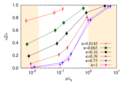
Figure 1: Time-averaged carrying capacity $Z$ versus the non-dimensional growth rate $\mu\tau_{\eta}$ for different values of compressibility $\kappa$. Region with $\mu\tau_{\eta}<\tau_{\eta}/\tau_{L}$ and $\mu\tau_{\eta}>1$ has been shaded for visual aid. Here, $\tau_{L}\equiv L/\sqrt{E}$ is the box size time scale with $L=2\pi$ per10 .

For large values of the growth rate, i.e. $\tau_{g}\ll\tau_{\eta}$, the time-scales of turbulence are too slow to have any effect on the evolution of the concentration, and $Z\to 1$.

In the limit $\tau_{g}\to 0$, the concentration field tends to become uniform with the leading correction coming from the local compressibility. After a series expansion one obtaines $\langle Z\rangle_{\mu}\approx 1-(\tau_{g}^{2}/L^{2})\langle\int({\bm{\nabla}}\cdot{\bf u})^{2}{\rm{d\bf x}}\rangle+{\cal O}(\tau_{g}^{3})$. The limiting values for small growth rates are complicated to access numerically, especially for $\kappa<0.16$, as it takes a longer and longer time for the carrying capacity to reach a steady state at decreasing $\mu=\tau_{g}^{-1}$. To obtain reliable estimates in this limit we can proceed as suggested in  per10

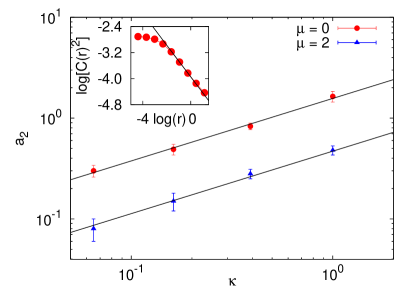
Figure 2: Log-log plot of the anomalous scaling exponent $a_{2}$ as a function for the compressibility $\kappa$ in the case $\mu=0$ and $\mu=2$. Note that the two scaling laws have the same slope with different offset. Inset: Scaling behavior of $\langle C^{2}_{\mu}(r)\rangle$ for $\mu=0$ and $\kappa=0.16$.

where it was shown using a multifractal analysis that as $\mu\to 0$ the statistics of $c$ closely resembles the statistics of the corresponding passive scalar probability density $P({\bm{x}},t)$, which satisfies Eq. (1) with $\mu=0$. The limiting values of $Z_{\mu\to 0}$ for different values of compressibility is given in Table 1.

The spatial behavior of $c({\bm{x}},t)$ is characterized by strong fluctuations with non trivial correlations in both space and time. In per10 it was shown that the multifractal analysis describes the statistical properties of the concentration field. Here we extend the analysis to different values of the compressibility, $\kappa$, and of the growth rate, $\mu$. We focus on the scaling of:

$$C^{q}_{\mu}(r)=\frac{1}{r^{2}}\left<\int_{B(r)}c(x,t)^{q}d^{2}x\right>$$ (3)

where $\langle\dots\rangle$ now stands for a time and ensemble average and $B(r)$ is a disk of radius $r$. Within the inertial range, we find that $C_{\mu}^{q}(r)\sim r^{-a_{q}}$ with $a_{q}$ a non linear function of $q$ constrained to $a_{0}=a_{1}=0$ roberto ; frisch (in the inset of Figure 2 we show the scaling of $C_{\mu}^{2}(r)$ versus $r$ for a particular value of $\mu=0$ and $\kappa=0.16$; plots for other values look similar). It is important to remember that each $\kappa>0$ can be associated with a compressibility length (and time) scale, $l_{\kappa}=u_{rms}/\langle{(\nabla\cdot u)}^{2}\rangle^{1/2}$ where $u_{rms}=\sqrt{E}$ is the root-mean-square velocity. For very small compressibilities, this scale will be comparable or larger than the integral scale of turbulence and the system can effectively be considered as incompressible. In our system this happened roughly for values of $\kappa<0.065$ and indeed for these compressibility values no scaling can be detected, making it impossible to compute $a_{q}$. Hereafter we limit our analysis to the region $\kappa\geq 0.065$.

We expect the scaling exponent $a_{2}$ to be a function of $\mu$, $\tau_{\eta}$ and $\kappa$. Using dimensional analysis, we expect that $a_{2}$ depends on $\mu$ and $\tau_{\eta}$ through the dimensionless combination $\mu\tau_{\eta}$ and that the time scale associated to the velocity gradient in the turbulent flow with compressibility $\kappa$, should be given by $1/\langle(\nabla\cdot\bf u)^{2}\rangle^{1/2}=\tau_{\eta}/\sqrt{\kappa}$. Hence, we conjecture that $a_{2}$ should depend only on the dimensionless combination $\sqrt{\kappa}/\mu\tau_{\eta}$. Since for $\mu=0$ we find that $a_{2}$ has a finite value for any value of compressibility $\kappa$, we further conjecture that $a_{2}\propto\sqrt{\kappa}/{(\mu\tau_{\eta}+\beta)}$ where $\beta$ is a constant. We expect that $\beta\approx\tau_{\eta}/\tau_{L}\approx 1/{Re_{\lambda}}$, where $\tau_{L}$ is the large eddy turnover time discussed above.

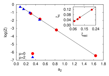
Figure 3: Logarithmic plot of the carrying capacity $Z$ versus the anomalous exponent $a_{2}(\kappa)$ for $\mu=0$ and $\mu=2$. The black line represent a best fit with slope $-3.9\pm 0.1$. We fit the data separately through $\mu=0$ and $\mu=2$ datasets. The mean of the fits is the slope and the error is the maximum deviation of the fit from the two slopes. Inset shows the linear relationship between the localization length and the estimated cut-off length for $Sc=0.1,0.5,1$, and $10$. The black line represents the best fit and has a slope $\approx 0.6$.

In Fig. 2, we show the scaling exponent $a_{2}$ for $\mu=0$ and $\mu=2$ and for different compressibilities $\kappa$. The most striking feature of Fig. 2 is the well defined scaling law between $a_{2}$ and $\kappa$ and that the scaling exponent does not change by changing $\mu\tau_{\eta}$. Therefore we can write:

$$a_{2}(\kappa,\mu\tau_{\eta})=a(\mu\tau_{\eta})\kappa^{\gamma}$$ (4)

where $a(\mu\tau_{\eta})=\alpha/(\mu\tau_{\eta}+\beta)$. Using the data in Fig. 2 we obtain $\gamma=0.62$, reasonably close to the prediction $\gamma=0.5$ given by dimensional analysis. Note that the function $a(\mu\tau_{\eta})$ in Eq. (4) is a decreasing function of $\mu\tau_{\eta}$, and that $\lim_{\mu\tau_{\eta}\to 0}a_{2}(\mu\tau_{\eta})=a_{2}(0)>0$.

In Ref. per10 it was shown that for $\mu=0$, the carrying capacity is related to $a_{2}$ by $Z\approx(\xi_{0}/L)^{a_{2}}$ where $\xi_{0}^{2}\equiv\langle P^{2}\rangle/\langle(\nabla P)^{2}\rangle$ and $P({\bm{x}},t)$ is the solution of Eq. (1) with $\mu=0$. Here we generalize the results of Ref.per10 for $\mu\neq 0$ and compressibilities $\kappa$ (see Table. 1). In Fig. 3 we plot $\log(Z)$ versus $a_{2}(\mu\tau_{\eta},\kappa)$ for $\mu=0$ and $\mu=2$, which supports the scaling ansatz

$$Z(\mu,\tau_{\eta},\kappa)=\left(\frac{\xi_{est}}{L}\right)^{a_{2}(\mu\tau_{\eta},\kappa)}$$ (5)

which defines the length scale $\xi_{est}$. In order to gain a deeper physical insight into the meaning of the cutoff scale $\xi_{est}$ we define a scale based on the gradient of the concentration field which is a generalization of our previous definition of $\xi_{0}$:

$$\xi_{c}^{2}=\frac{\langle c^{2}\rangle}{\langle(\nabla c)^{2}\rangle}.$$ (6)

In the inset of Fig. 3 we show the behavior of the two length scales $\xi_{est}$ and $\xi_{c}$ by varying the Schmidt number $0.1\leq Sc\leq 10$. Evidently the two definitions are consistent within a numerical prefactor, suggesting that $\xi_{est}$ is proportional to the cutoff scale of the gradients of the concentration field.

We can now test for a universal scaling behavior of the carrying capacity for varying compressibility $\kappa$ and non-dimensional growth rate $\mu\tau_{\eta}$ using Eq. 5.

Upon defining the quantity $X\equiv\log(a(\mu\tau_{\eta})\kappa^{\gamma})$ the validity of Eq. (5) can be checked by replotting the data of Fig. 1 for $Z$ as a function of $X$. Since $X=\log(\alpha)+\log[\kappa^{\gamma}/(\mu\tau_{\eta}+\beta)]$ and $\gamma=0.62$ from Fig. 2, data collapse of the results shown in Fig. 1 should hold for some particular value of $\beta$ whereas the exact value of $\alpha$ represents just a horizontal shift in the whole data set. In Fig. 4 we show that for $\beta=0.1$ all the data collapse on a well defined curve which represents our universal function. This estimate $\beta=0.1$ obtained for the data collapse is very close to the dimensional estimate $\beta\approx\tau_{\eta}/\tau_{L}\approx 0.02-0.03$ (shaded region on the left in Fig. 1). This result is important since it shows the deep and highly non-trivial connection between a bulk property of the system, namely $Z$, and the intermittency parameters of the FKPP equation in compressible flows. Moreover, Fig. 4 represents a prediction of the average carrying capacity covering an entire parameter space spanned by the three basic quantities of the system, namely $\mu$, $\kappa$ and $\tau_{\eta}$. Our numerical results can thus be extrapolated to new regimes, to investigate the importance of weak compressibility due, for instance, to inertial effects or buoyancy forces in populations subject to oceanic turbulence.

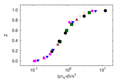
Figure 4: Semi-logarithmic plot of $Z$ as a function of $(\mu\tau_{\eta}+\beta)/\kappa^{\gamma}$ where $\gamma=0.62$ is given by the fit of Fig. 2 and $\beta=0.1$. All the data of Fig. 1 has been collapsed on a single curve.

In summary, we have used the FKPP equation to numerically study the population dynamics in a compressible turbulent velocity field. As a simplified model relevant for marine biology we have considered microorganisms (bacteria or plankton) confined to a two-dimensional plane experiencing the effect of a three dimensional velocity field. We have investigated in detail the effect of compressibility in a velocity field over a wide range of $\kappa$’s. We found that even a small compressibility can significantly reduce a global quantity like the average carrying capacity, due to the slow reproduction rate of the organisms. We expect that in oceans or lake this may be a common situation. We further quantified in terms of spatial intermittency exponents the statistical properties of the concentration field. Our study clearly suggests that it is quantitatively wrong to neglect even small degrees of effective compressibility. This compressibility, even in absence of organisms with active buoyancy control, can be induced by density mismatches or by the finite size of the organisms. Experimental tests of our findings would be of primary importance.

Acknowledgment We thank L. Biferale, H.J.H. Clercx, M.H. Jensen and S. Pigolotti for useful discussions. We acknowledge computational support from CASPUR (Roma, Italy under HPC Grant 2009 N. 310), from CINECA (Bologna, Italy) and SARA (Amsterdam, The Netherlands). Support for D.R.N. was provided in part by the National Science Foundation through Grant No. DMR-1005289 and by the Harvard Materials Research Science and Engineering Center through NSF Grant DMR-0820484. We acknowledge the COST Action MP0806 for support. PP and FT acknowledge the Kavli Institute of Theoretical Physics for hospitality. This research was supported in part by the National Science Foundation under Grant No. NSF PHY05-51164. Data from this study are publicly available in unprocessed raw format from the iCFDdatabase (http://cfd.cineca.it).

References

- (1) R. Fisher, Ann. Eugenics 7, 335 (1937); A. Kolmogorov, I. Petrovsky and N. Psicounoff, Moscow, Univ. Bull. Math. 1, 1 (1937).
- (2) J. Wakita et al., J. Phys. Soc. Jpn. 63, 1205 (1994).
- (3) R. Benzi and D. Nelson, Physica D 238, 2003 (2009).
- (4) P. Perlekar, R. Benzi, D. Nelson, and F. Toschi, Phys. Rev. Lett. 105, 144501 (2010).
- (5) F. Toschi and E. Bodenschatz, Ann. Rev. Fluid. Mech. 41, 1 (2009).
- (6) L. Moore, R. Goerrcke, and S. Chisholm, Mar. Ecol. Prog. Ser. 116, 259 (1995).
- (7) W. McKiver and Z. Neufeld, Phys. Rev. E 79, 061902 (2009).
- (8) A. Martin, Prog. in Oceanography 57, 125 (2003).
- (9) R. Benzi and L. Biferale, J. Stat. Phys. 135, 977 (2009).
- (10) U. Frisch, Turbulence: The Legacy of A.N. Kolmogorov (Cambridge University Press, Cambridge, 1996).