Tropical geometries and dynamics of biochemical networks. Application to hybrid cell cycle models.

Abstract

We use the Litvinov-Maslov correspondence principle to reduce and hybridize networks of biochemical reactions. We apply this method to a cell cycle oscillator model. The reduced and hybridized model can be used as a hybrid model for the cell cycle. We also propose a practical recipe for detecting quasi-equilibrium QE reactions and quasi-steady state QSS species in biochemical models with rational rate functions and use this recipe for model reduction. Interestingly, the QE/QSS invariant manifold of the smooth model and the reduced dynamics along this manifold can be put into correspondence to the tropical variety of the hybridization and to sliding modes along this variety, respectively

Keywords: systems biology, model reduction, hybrid models, tropical geometry

1 Introduction.

Systems biology develops biochemical dynamic models of various cellular processes such as signalling, metabolism, gene regulation. These models can reproduce complex spatial and temporal dynamic behavior observed in molecular biology experiments. In spite of their complex behavior, currently available dynamical models are relatively small size abstractions, containing only tens of variables. This modest size results from the lack of precise information on kinetic parameters of the biochemical reactions on one hand, and of the limitations of parameter identification methods on the other hand. Further limitations can result from the combinatorial explosion of interactions among molecules with multiple modifications and interaction sites [DFF⁺07]. In middle out modeling strategies small models can be justified by saying that one looks for an optimal level of complexity that captures the salient features of the phenomenon under study. The ability to choose the relevant details and to omit the less important ones is part of the art of the modeler. Beyond modeler’s art, the success of simple models relies on an important property of large dynamical systems. The dynamics of multiscale, dissipative, large biochemical models, can be reduced to that of simpler models, that were called dominant subsystems [RGZL08, GRZ10, GR08]. Simplified, dominant subsystems contain less parameters and are more easy to analyze. The choice of the dominant subsystem depends on the comparison among the time scales of the large model. Among the conditions leading to dominance and allowing to generate reduced models, the most important are quasi-equilibrium (QE) and the quasi-steady state (QSS) approximations [GRZ10]. In nonlinear systems, timescales and together with them dominant subsystems can change during the dynamics and undergo more or less sharp transitions. The existence of these transitions suggests that a hybrid, discrete/continous framework is well adapted for the description of the dynamics of large nonlinear systems with multiple time scales [CDR09, NVR10, NVR11].

The notion of dominance can be exploited to obtain simpler models from larger models with multiple separated timescales and to assemble these simpler models into hybrid models. This notion is asymptotic and a natural mathematical framework to capture multiple asymptotic relations is the tropical geometry. Motivated by applications in mathematical physics [LM96], systems of polynomial equations [Stu02], etc., tropical geometry uses a change of scale to transform nonlinear systems into discontinuous piecewise linear systems. The tropicalization is a robust property of the system, remaining constant for large domains of parameter values; it can reveal qualitative stable features of the system’s dynamics, such as various types of attractors. Thus, the use of tropicalization to model large systems in molecular biology could be a promising solution to the problem of incomplete or imprecise information on the kinetic parameters.

In this paper we propose a method for reduction and hybridization of biochemical networks. This method, based on tropical geometry, could be used to automatically produce the simple models that are needed in middle-out approaches of systems biology.

2 Biochemical networks with rational rate functions.

Systems biology models use the formalism of chemical kinetics to model dynamics of cellular processes. We consider here that the molecules of various species are present in sufficient large numbers and that stochastic fluctuations are negligible as a consequence of the law of large numbers and/or of the averaging theorem [CDR09]. We also consider that space transport phenomena are sufficiently rapid such that the well stirred reactor hypothesis is valid. In these conditions, the dynamics of the biochemical system can be described by systems of differential equations. In chemical kinetics, enzymatic reactions are often presented as indivisible entities characterized by stoichiometry vectors and rate functions. However, each enzymatic reaction can be decomposed into several steps that define the reaction mechanism. The resulting stoichiometry and global rate depend on the mechanism. Several methods were designed for calculating effective rates of arbitrarily complex mechanisms. For linear mechanisms King and Altman [KA56] proposed a graphical method to compute global rates; these are rational functions of the concentrations (an example is the Michaelis-Menten equation). Yablovsky and Lazman [LY08b] studied the same problem for non-linear mechanisms and found that in this case the reaction rates are solutions of polynomial equations; these can be solved by radicals in a few number of cases and can be calculated by multi-variate hypergeometric series in general [LY08b]. Truncation of these series to finite order leads to rational approximations of the reaction rates.

In chemical kinetics with rational reaction rates the concentration $x_{i}$ of the $i$-th component follows the ordinary differential equation:

$$\frac{dx_{i}}{dt}=P_{i}(\mathbold x)/Q_{i}(\mathbold x),$$ (1)

where $P_{i}(\mathbold x)=\sum_{\alpha\in A_{i}}a_{i,\alpha}\mathbold x^{\alpha}$, $Q_{i}(\mathbold x)=\sum_{\beta\in B_{i}}b_{i,\beta}\mathbold x^{\beta}$, are polynomials and we have $1\leq i\leq n$. Here $\mathbold x^{\alpha}=x_{1}^{\alpha_{1}}x_{2}^{\alpha_{2}}\ldots x_{n}^{\alpha_{n}}$, $\mathbold x^{\beta}=x_{1}^{\beta_{1}}x_{2}^{\beta_{2}}\ldots x_{n}^{\beta_{n}}$, $a_{i,\alpha},b_{i,\beta}$, are nonzero real numbers, and $A_{i},B_{i}$ are finite subsets of ${\mathbb{N}}^{n}$ called supports of $P_{i}$ and $Q_{i}$.

A simple example of model with rational reaction rates is the minimal cell cycle oscillator model proposed by Tyson [Tys91]. This example will be studied throughout the paper. The dynamics of this nonlinear model that contains 5 species and 7 reactions is described by a system of 5 polynomial differential equations:

$$y_{1}^{\prime} =k_{9}y_{2}-k_{8}y_{1}+k_{6}y_{3},$$

$$y_{2}^{\prime} =k_{8}y_{1}-k_{9}y_{2}-k_{3}y_{2}y_{5},$$

$$y_{3}^{\prime} =k_{4}^{\prime}y_{4}+k_{4}y_{4}y_{3}^{2}/C^{2}-k_{6}y_{3},$$

$$y_{4}^{\prime} =-k_{4}^{\prime}y_{4}-k_{4}y_{4}y_{3}^{2}/C^{2}+k_{3}y_{2}y_{5},$$

$$y_{5}^{\prime} =k_{1}-k_{3}y_{2}y_{5},$$ (2)

where $$y_{1}+y_{2}+y_{3}+y_{4}=C.$$

3 Hybridization and tropical geometry.

Tropical geometry is a new branch of algebraic geometry that studies the asymptotic properties of varieties. While algebraic geometry deals with polynomial functions, tropical geometry deals with piecewise linear functions with integer directing slopes. Tropical geometry has a growing number of applications in enumerative problems in nonlinear equation solving [Roj03], statistics [PS04], traffic optimization [Aub10].

The logarithmic transformation $u_{i}=logx_{i},\,1\leq i\leq n$, well known for drawing graphs on logarithmic paper, plays a central role in tropical geometry [Vir08]. By abus de langage, here we call logarithmic paper the image of ${\mathbb{R}}^{n}_{+}$ by the logarithmic transformation, even if $n>2$. Monomials $M(\mathbold x)=a_{\alpha}\mathbold x^{\alpha}$ with positive coefficients $a_{\alpha}>0$, become linear functions, $logM=loga_{\alpha}+<\alpha,log(\mathbold x)>$, by this transformation. Furthermore, the euclidian distance on the logarithmic paper is a good measure of separation (see next section).

Litvinov and Maslov [LMS01, LM96] proposed a heuristic (correspondence principle) allowing to transform mathematical objects (integrals, polynomials) into their quantified (tropical) versions. According to this heuristic, to a polynomial with positive real coefficients $\sum_{\alpha\in A}a_{\alpha}\mathbold x^{\alpha}$, one associates the max-plus polynomial $max_{\alpha\in A}\{log(a_{\alpha})+<log(\mathbold x),\alpha>\}$.

We adapt this heuristic to associate a piecewise-smooth hybrid model to the systems of rational ODEs (1).

Definition 1

We call tropicalization of the smooth ODE system (1) the following piecewise-smooth system:

$$\frac{dx_{i}}{dt}=s_{i}exp[max_{\alpha\in A_{i}}\{log(|a_{i,\alpha}|)+<\mathbold u,\alpha>\}-max_{\beta\in B_{i}}\{log(|b_{i,\beta}|)+<\mathbold u,\beta>\}],$$ (3)

where $\mathbold u=(logx_{1},\ldots,logx_{n})$, $s_{i}=sign(a_{i,\alpha_{max}})sign(b_{i,\beta_{max}})$ and $a_{i,\alpha_{max}},\,\alpha_{max}\in A_{i}$ (respectively, $b_{i,\beta_{max}},\,\beta_{max}\in B_{i}$) denotes the coefficient of a monomial of the numerator (respectively, of the denominator) for which the maximum occurring in (3) is attained.

In a different notation this reads:

$$\frac{dx_{i}}{dt}=Dom\{a_{i,\alpha}\mathbold x^{\alpha}\}_{\alpha\in A_{i}}/Dom\{b_{i,\beta}\mathbold x^{\beta}\}_{\alpha\in B_{i}},$$ (4)

where $Dom\{a_{i,\alpha}\mathbold x^{\alpha}\}_{\alpha\in A_{i}}=sign(a_{i,\alpha_{max}})exp[max_{\alpha\in A_{i}}\{log(|a_{i,\alpha}|)+<\mathbold u,\alpha>\}]$.

Finally, the tropicalization can be written with Heaviside functions:

$$\frac{dx_{i}}{dt}=\frac{\sum_{\alpha\in A_{i}}a_{i,\alpha}\mathbold x^{\alpha}\prod_{\alpha^{\prime}\neq\alpha}\theta(<\alpha-\alpha^{\prime},log(\mathbold x)>+log(|a_{i,\alpha}|)-log(|a_{i,\alpha^{\prime}}|))}{\sum_{\beta\in B_{i}}b_{i,\beta}\mathbold x^{\beta}\prod_{\beta^{\prime}\neq\beta}\theta(<\beta-\beta^{\prime},log(\mathbold x)>+log(|b_{i,\beta}|)-log(|b_{i,\beta^{\prime}}|))},$$ (5)

where $\theta(x)=1$ if $x>0$, $0$ if not.

The following definitions are standard and will be used throughout the paper:

Definition 2

The Newton polytope of a polynomial $P(\mathbold x)=\sum_{\alpha\in A}a_{\alpha}\mathbold x^{\alpha}$ is defined as the convex hull of the support of $P$, $New(P)=conv(A)$.

Definition 3

The max-plus polynomial $P^{\tau}(\mathbold x)=max\{log|a_{\alpha}|+<\alpha,log(\mathbold x)>\}$ is called the tropicalization of $P(\mathbold x)$. The logarithmic function is defined as $log(\mathbold x):{\mathbb{R}}_{+}^{n}\to{\mathbb{R}}^{n}$, $log(\mathbold x)_{i}=log(x_{i})$.

Definition 4

The set of points $\mathbold x\in{\mathbb{R}}^{n}$ where $P^{\tau}(\mathbold x)$ is not smooth is called tropical variety. Alternative names are used such as logarithmic limit sets, Bergman fans, Bieri-Groves sets, or non Archimedean amoebas [PT05].

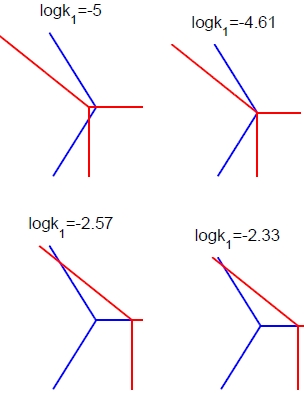
In two dimensions, a tropical variety is a tropical curve made of several half-lines (tentacles) and finite intervals [Mik]. A tropical line corresponds to only three monomials and is made of three half lines sharing a common point. The tentacles and the intervals of the tropical variety are orthogonal to the edges and point to the interior of the Newton polygon [PT05] (see Fig.1).

4 Dominance and separation.

The above heuristic is related to the notion of dominance. Actually we have replaced each polynomial in the rational function by the dominant monomial. Dominance of monomials has an asymptotic meaning inside cones of the logarithmic paper. For instance ${\mathbold x}^{\alpha}$ dominates ${\mathbold x}^{\beta}$ on the half plane $<log(\mathbold x),\alpha-\beta>>0$ of the logarithmic paper. We have ${\mathbold x}^{\beta}/{\mathbold x}^{\alpha}\to 0$ when the limit is taken along lines in this half plane.

For practical applications, we would also need a finite scale notion of dominance.

Let $M_{1}(\mathbold x)=a_{\alpha_{1}}\mathbold x^{\alpha_{1}}$ and $M_{2}(\mathbold x)=a_{\alpha_{2}}\mathbold x^{\alpha_{2}}$ be two monomials. We define the following binary relations:

Definition 5 (Separation)

$M_{1}$ and $M_{2}$ are separated on a domain $D\subset R^{n}_{+}$ at a level $\rho>0$ if $|log(|a_{\alpha_{1}}|\mathbold x^{\alpha_{1}})-log(|a_{\alpha_{2}}|\mathbold x^{\alpha_{2}})|>\rho$ for all $\mathbold x\in D$.

On logarithmic paper, two monomials are separated on the domain $D$, if $D$ is separated by the euclidian distance $\rho$ from the hyperplane $<log(\mathbold x),\alpha_{1}-\alpha_{2}>=log|a_{\alpha_{2}}|-log|a_{\alpha_{1}}|$.

Definition 6 (Dominance)

The monomial $M_{1}$ dominates the monomial $M_{2}$ at the level $\rho>0$, $M_{1}\succ_{\rho}M_{2}$, if $log(|a_{\alpha_{1}}|\mathbold x^{\alpha_{1}})>log(|a_{\alpha_{2}}|\mathbold x^{\alpha_{2}})+\rho$ for all $\mathbold x\in D\subset{\mathbb{R}}_{+}^{n}$.

Dominance is a partial order relation on the set of multivariate monomials defined on subsets of ${\mathbb{R}}_{+}^{n}$.

5 Dominance and global reduction of large models.

There are two simple methods for model reduction of nonlinear models with multiple timescales: the quasi-equilibrium (QE) and the quasi-steady state (QSS) approximations. As discussed in [GRZ10], these two approximations are physically and dynamically distinct. Here we present a method allowing to detect QE reactions and QSS species.

Like in [RGZL08], the first step of the method is to detect the ”slaved” species, i.e. the species that obey quasi-steady state equations. These can be formally defined by introducing the notion of imposed trace. Given the traces $\mathbold x(t)$ of all the species, the imposed trace of the $i$-th species is a real solution $x_{i}^{*}(t)$ of the polynomial equation $P_{i}(x_{1}(t),\ldots,x_{i-1}(t),x_{i}^{*}(t),x_{i+1}(t),\ldots,x_{n}(t))=0$. Eventually, there may be several imposed traced, because a polynomial equation can have several real solutions.

Definition 7

We say that a species is slaved if the distance between the traces $x_{i}(t)$ and some imposed trace $x_{i}^{*}(t)$ is small on some interval, $sup_{t\in I}|log(x_{i}(t))-log(x_{i}^{*}(t))|<\delta$, for some $\delta>0$ sufficiently small. A species is globally slaved if $I=(T,\infty)$ for some $T\geq 0$.

Slaved species are good candidates for QSS species and this criterion was used to identify QSS species in [RGZL08]. More generally, slaved species are involved in rapid processes, but are not always QSS. Actually, two distinct cases lead to slaved species.

Quasi-equilibrium. A system with fast, quasi-equilibrium reactions has the following structure [GRZ10]:

$$\frac{d\mathbold x}{dt}=\sum_{s,slow}R_{s}(\mathbold x)\mathbold\gamma^{s}+\frac{1}{\epsilon}\sum_{f,fast}R_{f}(\mathbold x)\mathbold\gamma^{f},$$ (6)

where $\epsilon>0$ is a small parameter $\mathbold\gamma^{s},\mathbold\gamma^{f}\in{\mathbb{Z}}^{n}$ are stoichiometric vectors. The reaction rates $R_{s}(\mathbold x)$, $R_{f}(\mathbold x)$ are considered rational functions of $\mathbold x$.

To separate slow/fast variables, we have to study the spaces of linear conservation law of the initial system (6) and of the following fast subsystem:

$$\frac{d\mathbold x}{dt}=\frac{1}{\epsilon}\sum_{f,fast}R_{f}(\mathbold x)\mathbold\gamma^{f}.$$ (7)

In general, the system (6) can have several conservation laws. These are linear functions $b^{1}(\mathbold x),\ldots,b^{m}(\mathbold x)$ of the concentrations that are constant in time. The conservation laws of the system (7) provide variables that are constant on the fast timescale. If they are also conserved by the full dynamics, the system has no slow variables (variables are either fast or constant). In this case, the dynamics of the fast variables is simply given by Eq.(7). Suppose now that the system (7) has some more conservation laws $b^{m+1}(\mathbold x),\ldots,b^{m+l}(\mathbold x),$ that are not conserved by the full system (6). Then, these provide the slow variables of the system. The fast variables are those $x_{i}$ such that $(\mathbold\gamma^{f})_{i}\neq 0$, for some fast reaction $f$.

Let us suppose that the fast system (7) has a stable steady state that is a solution of the QE equations (augmented by the conservation laws of the fast system):

$$\sum_{f,fast}R_{f}(\mathbold x)\mathbold\gamma^{f}=0,$$ (8)

$$b^{i}(\mathbold x)=C_{i},\quad 1\leq i\leq m+l.$$ (9)

By classical singular perturbation methods [TVS85, Was65] one can show that the fast variables can be decomposed as $x_{i}=\tilde{x}_{i}+\eta_{i}$ where $\tilde{x}_{i}$ satisfy the QE equations (8) and $\eta_{i}={\cal O}(\epsilon)$, meaning that the fast variables $x_{i}$ are slaved [GRZ10].

Let $P_{i}$, $\tilde{P}_{i}$ be the numerators of the rational functions $\sum_{s,slow}R_{s}(\mathbold x)\mathbold\gamma^{s}_{i}+\frac{1}{\epsilon}\sum_{f,fast}R_{f}(\mathbold x)\mathbold\gamma^{f}_{i}$ and $\sum_{f,fast}R_{f}(\mathbold x)\mathbold\gamma^{f}_{i}$, respectively. We call $\tilde{P}_{i}$ the pruned version of $P_{i}$. When $\epsilon$ is small enough, the monomials of the pruned version $\tilde{P}_{i}$ dominate the monomials of $P_{i}$. This suggests a practical recipe for identifying QE reactions:

Algorithm 1

Step 1: Detect slaved species.

Step 2: For each $P_{i}$ corresponding to slaved species, compute the pruned version $\tilde{P}_{i}$ by eliminating all monomials that are dominated by other monomials of $P_{i}$.

Step 3: Identify, in the structure of $\tilde{P}_{i}$ the forward and reverse rates of QE reactions. This step could be performed by recipes presented in [SH10].

Quasi-steady state. In the most usual version of QSS approximation [SS89], the species are split in two groups with concentration vectors $\mathbold x^{s}$ (“slow” or basic components) and $\mathbold x^{f}$ (“fast” or QSS species).

Quasi-steady species (also called radicals or fast intermediates) are low-concentration, slaved species. Typically, QSS species are consumed (rather than produced) by fast reactions. The small parameter $\epsilon$ used in singular perturbation theory is now the ratio of small concentrations of fast intermediates to the concentration of other species. After rescaling $\mathbold x^{s}$ and $\mathbold x^{f}$ to order one, the set of kinetic equations reads:

$$\frac{d\mathbold x^{s}}{dt} =\mathbold W^{s}(\mathbold x^{s},\mathbold x^{f}),$$ (10)

$$\frac{d\mathbold x^{f}}{dt} =(1/\epsilon)\mathbold W^{f}(\mathbold x^{s},\mathbold x^{f}),$$ (11)

where the functions $\mathbold W^{s}$, $\mathbold W^{f}$ and their derivatives are of order one ($0<\epsilon<<1$).

Let us suppose that the fast dynamics (11) has a stable steady state. The standard singular perturbation theory[TVS85, Was65] provides the QSS algebraic condition $\mathbold W^{f}(\mathbold x^{s},\mathbold x^{f})=0$ which means that fast species $\mathbold x^{f}$ are slaved. These equations, together with additional balances for $x^{f}$ (conservation laws) are enough to deduce the fast variables $x^{f}$ as functions of the slow variables $x^{s}$ and to eliminate them [YBGE91, LY08a, RGZL08]. The slow dynamics is given by Eq.(10).

In networks with rational reaction rates the components of $\mathbold W^{f}(\mathbold x^{s},\mathbold x^{f})$ are rational functions. Like for QE we can define $P_{i}$ as numerators of $\mathbold W^{f}_{i}$. The difference between QSS conditions with respect to QE situation is that in the pruned polynomial $\tilde{P}_{i}$ one can no longer find forward and backward rates of QE reactions, ie the step 3 of Algorithm 1 will not identify reversible reactions. Alternatively, one can realize that slaved species can have relatively large concentrations, in which case they are not QSS species. However, it is difficult to say which concentration value separates QSS from non QSS species among slaved species, hence the former, qualitative criterion is better.

6 Sliding modes of the tropicalization.

A notable phenomenon resulting from tropicalization is the occurrence of sliding modes. Sliding modes are well known for ordinary differential equations with discontinuous vector fields [FA88]. In such systems, the dynamics can follow discontinuity hypersurfaces where the vector field is not defined.

The conditions for the existence of sliding modes are generally intricate. However, when the discontinuity hypersurfaces are smooth and $n-1$ dimensional ($n$ is the dimension of the vector field) then the conditions for sliding modes read:

$$<n_{+}(x),f_{+}(x)><0,\quad<n_{-}(x),f_{-}(x)><0,\quad x\in\Sigma,$$ (12)

where $f_{+},f_{-}$ are the vector fields on the two sides of $\Sigma$ and $n_{+}=-n_{-}$ are the interior normals.

Let us consider that the smooth system (1) has quasi-steady state species or quasi-equilibrium reactions. In this case, the fast dynamics reads:

$$\frac{dx_{i}}{dt}=\frac{1}{\epsilon}\tilde{P}_{i}(\mathbold x)/\tilde{Q}_{i}(\mathbold x),\quad i\quad\text{fast},$$ (13)

where $\tilde{P}_{i}(\mathbold x)$, $\tilde{Q}_{i}(\mathbold x)$ are pruned versions of $P_{i}$, $Q_{i}$, and $\epsilon$ is the small, singular perturbation parameter.

For sufficiently large times, the fast variables satisfy (to ${\cal O}(\epsilon)$):

$$\tilde{P}_{i}(\mathbold x)=0,\quad i\quad\text{fast}.$$ (14)

The pruned polynomial is usually a fewnomial (contains a small number of monomials). In particular, let us consider the case when only two monomials remain after pruning, $\tilde{P}_{i}(\mathbold x)=a_{1}\mathbold x^{\alpha_{1}}+a_{2}\mathbold x^{\alpha_{2}}$. Then, the equation (14) defines a hyperplane $S=\{<log(\mathbold x),\alpha_{1}-\alpha_{2}>=log(|a_{1}|/|a_{2}|)\}$. This hyperplane belongs to the tropical variety of $\tilde{P}_{i}$, because it is the place where the monomial $\mathbold x^{\alpha_{1}}$ switches to $\mathbold x^{\alpha_{2}}$ in the max-plus polynomial defined by $\tilde{P}_{i}$. For $\epsilon$ small, the QE of QSS conditions guarantee the existence of an invariant manifold ${\mathcal{M}}_{\epsilon}$, whose distance to $S$ is ${\cal O}(\epsilon)$.

Let $n_{+},n_{-}$ defined as above and let $(f_{+})_{i}=\frac{1}{\tilde{Q}_{i}(\mathbold x)}a_{1}\mathbold x^{\alpha_{1}}$, $(f_{-})_{i}=\frac{1}{\tilde{Q}_{i}(\mathbold x)}a_{2}\mathbold x^{\alpha_{2}}$, $f_{i}=\frac{1}{\epsilon}[(f_{+})_{i}+(f_{-})_{i}]$ for $i$ fast, $(f_{+})_{j}=(f_{-})_{j}=f_{j}=\frac{\tilde{P}_{j}}{\tilde{Q}_{j}}$, for $j$ not fast. Then, the stability conditions for the invariant manifold read $<n_{+}(x_{+}),f(x_{+})><0$, $<n_{-}(x_{-}),f(x_{-}))><0$, where $x_{+},x_{-}$ are close to ${\mathcal{M}}_{\epsilon}$ on the side towards which points $n_{+}$ and $n_{-}$, respectively. We note that $|(f_{+})_{i}(x_{+})|>|(f_{-})_{i}(x_{+})|$. Thus, $<n_{+},f>=\frac{1}{\epsilon}(n_{+})_{i}[(f_{+})_{i}+(f_{-})_{i}]+\sum_{j,notfast}(n_{+})_{j}(f_{+})_{j}$ and $<n_{+},f_{+}>=\frac{1}{\epsilon}(n_{+})_{i}(f_{+})_{i}+\sum_{j,notfast}(n_{+})_{j}(f_{+})_{j}$. Thus, if $<n_{+},f><0$, then for $\epsilon$ small enough $(n_{+})_{i}(f_{+})_{i}<0$ and $<n_{+},f_{+}><0$ because $<n_{+},f>><n_{+},f_{+}>$. Similarly, we show that $<n_{-},f><0$ implies $<n_{-},f_{-}><0$. This proves the following

Theorem 1

If the smooth dynamics obeys QE or QSS conditions and if the pruned polynomial $\tilde{P}$ defining the fast dynamics is a 2-nomial, then the QE or QSS equations define a hyperplane of the tropical variety of $\tilde{P}$. The stability of the QE of QSS manifold implies the existence of a sliding mode of the tropicalization along this hyperplane.

The converse result, i.e. deducing the stability of the QE/QSS manifold from the existence of a sliding mode on the tropical variety may be wrong. Indeed, it is possible for a trajectory of the smooth system to be close to a hyperplane of the tropical variety carrying a sliding mode and where the QE/QSS equations are satisfied identically. However, as we will see in the next section, this trajectory can leave the hyperplane sooner than the sliding mode.

Figure 1: (top left) Detection of slaved species by comparing traces to imposed traces: the species $y_{1},y_{2},y_{5}$ are slaved globally, the species $y_{3},y_{4}$ are slaved on intervals $Q_{3}$,$Q_{4}$, respectively. (top right) Comparison of monomials of the polynomial systems of quasi-steady state equations. (bottom left) Newton polygons and inner normals of the reduced two dimensional polynomial model. (bottom right) Phase portrait on logarithmic paper of the reduced two dimensional model. We represent the two tropical curves (the tripods graphs, a red and a blue one), the modes (smooth vector fields within domains bordered by tropical curves tentacles), the smooth and tropicalized limit cycles. The tropicalized cycle contains two sliding modes $S_{3}$,$S_{4}$ corresponding to the intervals $Q_{3}$, $Q_{4}$ on which $y_{3}$, $y_{4}$ are quasi-stationary, respectively.

7 From smooth to hybrid models via reduction.

Starting with the system (2) we first reduce it to a simpler model. The analysis of the model is performed for the values of parameters from [Tys91], namely $k_{1}=0.015,k_{3}=200,k_{4}=180,k_{4}^{\prime}=0.018,k_{6}=1,k_{7}=0.6,k_{8}=1000000,k_{9}=1000$;

In order to do that we generate one or several traces (trajectories) $y_{i}(t)$. The smooth system has a stable periodic trace which is a limit cycle attractor. We also compute the imposed traces $y_{i}^{*}(t)$ that are solutions of the equations:

$$k_{9}y_{2}(t)-k_{8}y_{1}^{*}(t)+k_{6}y_{3}(t)=0,$$

$$k_{8}y_{1}(t)-k_{9}y_{2}^{*}(t)-k_{3}y_{2}(t)y_{5}(t)=0,$$

$$k_{4}^{\prime}y_{4}(t)+k_{4}y_{4}(t)y_{3}^{*2}(t)/C^{2}-k_{6}y_{3}^{*}(t)=0,$$

$$-k_{4}^{\prime}y_{4}^{*}(t)-k_{4}y_{4}^{*}(t)y_{3}^{2}(t)/C^{2}+k_{3}y_{2}(t)y_{5}(t)=0,$$

$$k_{1}-k_{3}y_{2}(t)y_{5}^{*}(t)=0.$$ (15)

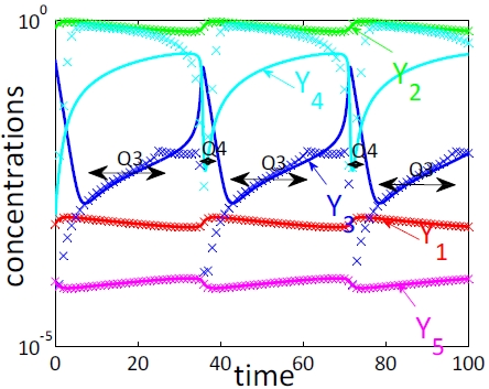
We find that, for three species $y_{1}$,$y_{2}$, and $y_{5}$, the distance between the traces $y_{i}^{*}(t)$ and $y_{i}(t)$ is small for all times which means that these species are slaved on the whole limit cycle (Figure 1 top left). Also, we have a global conservation law $y_{1}+y_{2}+y_{3}+y_{4}=C$, that can be obtained by summing the first four differential equations in (2). The three quasi-steady state equations for the three slaved species have to be solved jointly with the global conservation law:

$$k_{9}y_{2}-k_{8}y_{1}+k_{6}y_{3}=0,$$

$$k_{8}y_{1}-k_{9}y_{2}-k_{3}y_{2}y_{5}=0,$$

$$k_{1}-k_{3}y_{2}y_{5}=0,$$

$$y_{1}+y_{2}+y_{3}+y_{4}=C.$$ (16)

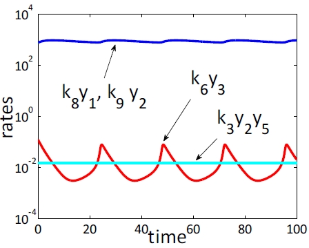
Comparison of the monomials (for values of parameters as above) in this system shows that $max(k_{8}y_{1},k_{9}y_{2})\succ k_{6}y_{3}$, and $max(k_{8}y_{1},k_{9}y_{2})\succ k_{3}y_{2}y_{5}$ (Fig.1 top right) which leads to the pruned system:

$$k_{8}y_{1}-k_{9}y_{2}=0,$$

$$k_{8}y_{1}-k_{9}y_{2}=0,$$

$$k_{1}-k_{3}y_{2}y_{5}=0,$$

$$y_{1}+y_{2}+y_{3}+y_{4}=C.$$ (17)

The first two equations are identical and correspond to quasi-equilibrium of the reaction between $y_{1}$ and $y_{2}$. The third equation means that $y_{5}$ is a quasi-steady state species. The pruned system allows the elimination of the variables $y_{1},y_{2},y_{5}$. The slow variable $y_{12}=y_{1}+y_{2}$ demanded by the quasi-equilibrium condition (this is a conservation law of the fast system) can be eliminated by using the global conservation law.

We note that the dominance relations leading to the pruned equations were found numerically in a neighborhood of the periodic trace. This means that QE and QSS approximations are valid at least on the limit cycle. More global testing of these relations will be presented elsewhere. Note that the system (16) can be solved also without pruning. However, (16) has four independent equations allowing to eliminate four of the five dynamic variables leading to a one dimensional dynamical system. It turns out that the correct application of the QE and QSS approximations has to use (17) and not (16).

After elimination, we obtain the following reduced differential-algebraic dynamical system:

$$y_{3}^{\prime} =k_{4}^{\prime}y_{4}+k_{4}y_{4}y_{3}^{2}/C^{2}-k_{6}y_{3},$$

$$y_{4}^{\prime} =-k_{4}^{\prime}y_{4}-k_{4}y_{4}y_{3}^{2}/C^{2}+k_{1},$$

$$y_{1} =(C-y_{3}-y_{4})k_{9}/(k_{8}+k_{9}),$$

$$y_{2} =(C-y_{3}-y_{4})k_{8}/(k_{8}+k_{9}),$$

$$y_{5} =k_{1}(k_{8}+k_{9})/(k_{3}k_{8}(C-y_{3}-y_{4}).$$ (18)

Now we tropicalize this reduced system. The tropicalization could have been done on the initial system in which case the pruned equations (17) would indicate that the reduced dynamics is a sliding mode of the tropicalized system on the two dimensional hypersurface $k_{8}y_{1}=k_{9}y_{2},k_{1}=k_{3}y_{2}y_{5},y_{1}+y_{2}+y_{3}+y_{4}=C$. However, although the result (concerning the dynamics on the QE/QSS manifold) should be the same, it is much handier to tropicalize the reduced system (18). Indeed, the tropicalization of the full 5D system is difficult to visualize and would also produce complex modes that can not be reduced to 2D (these modes describe the fast relaxation to the QE/QSS manifold).

The resulting hybrid model reads:

$$y_{3}^{\prime} =Dom\{k_{4}^{\prime}y_{4},k_{4}y_{4}y_{3}^{2}/C^{2},-k_{6}y_{3}\},$$

$$y_{4}^{\prime} =Dom\{-k_{4}^{\prime}y_{4},-k_{4}y_{4}y_{3}^{2}/C^{2},k_{1}\},$$

or equivalently using Heaviside functions:

$$y_{3}^{\prime} =k_{4}^{\prime}y_{4}\theta(-h_{1}-2u_{3})\theta(h_{2}+u_{4}-u_{3})+\frac{k_{4}}{C^{2}}y_{4}y_{3}^{2}\theta(h_{1}+2u_{3})\theta(h_{1}+h_{2}+u_{4}+u_{3})$$

$$-k_{6}y_{3}\theta(-h_{2}-u_{4}+u_{3})\theta(-h_{1}-h_{2}-u_{4}-u_{3}),$$

$$y_{4}^{\prime} =-k_{4}^{\prime}y_{4}\theta(-h_{3}-2u_{3})\theta(-h_{4}+u_{4})-\frac{k_{4}}{C^{2}}y_{4}y_{3}^{2}\theta(h_{3}+2u_{3})\theta(h_{3}-h_{4}+2u_{3}+u_{4})$$ (20)

$$k_{1}\theta(h_{4}-u_{4})\theta(-h_{3}+h_{4}-2u_{3}-u_{4}),$$

where $h_{1}=h_{3}=log(k_{4}/(k_{4}^{\prime}C^{2}))$, $h_{2}=log(k_{4}^{\prime}/k_{6})$, $h_{4}=log(k_{1}/k_{4}^{\prime})$.

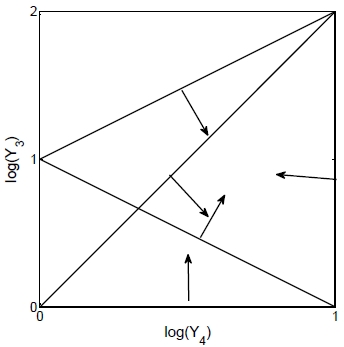
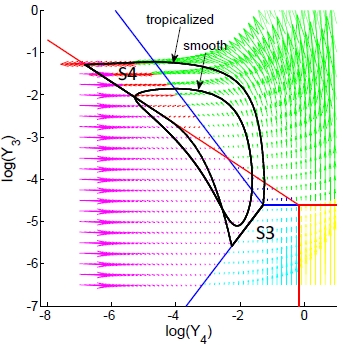
The Newton polygons of the polynomials $k_{4}^{\prime}y_{4}+k_{4}y_{4}y_{3}^{2}/C^{2}-k_{6}y_{3}$ and $-k_{4}^{\prime}y_{4}-k_{4}y_{4}y_{3}^{2}/C^{2}-k_{6}y_{3}$ are triangles (Fig.1 bottom left). The two triangles share a common edge which is a consequence of the fact that the reduced model have two reactions each one acting on the two species. The tentacles of the two tropical curves (in red and blue in Fig.1 bottom right) point in the same directions as the inner normals to the edges of the Newton polygons (the corresponding equations are $h_{1}+2u_{3}=0$, $h_{2}+u_{4}-u_{3}=0$, $h_{1}+h_{2}+u_{4}+u_{3}=0$ for one and $h_{3}+2u_{3}=0$, $h_{4}+u_{4}=0$, $h_{3}-h_{4}+2u_{3}+u_{4}=0$ for the other). These tentacles (half lines) decompose the positive quarter plane into 6 sectors corresponding to the 6 modes of the hybrid model.

In Fig.1 bottom right we have also represented the phase portrait of the reduced model on logarithmic paper. The dynamical variables are $u_{3}=log(y_{3})$ and $u_{4}=log(y_{4})$. The vector field corresponding to $u_{3}^{\prime}=y_{3}^{\prime}/y_{3}$ and $u_{4}^{\prime}=y_{4}^{\prime}/y_{4}$ was computed with the dominant monomials in each plane sector as follows:

$$u_{4}^{\prime} =-k_{4}y_{3}^{2},u_{3}^{\prime}=-k_{6}\text{ for the mode 1},$$

$$u_{4}^{\prime} =-k_{4}y_{3}^{2},u_{3}^{\prime}=k_{4}y_{3}y_{4}\text{ for the mode 2},$$

$$u_{4}^{\prime} =k_{1}y_{4}^{-1},u_{3}^{\prime}=k_{4}y_{3}y_{4}\text{ for the mode 3},$$

$$u_{4}^{\prime} =k_{1}y_{4}^{-1},u_{3}^{\prime}=k_{4}^{\prime}y_{4}y_{3}^{-1}\text{ for the mode 4},$$

$$u_{4}^{\prime} =k_{1}y_{4}^{-1},u_{3}^{\prime}=-k_{6}\text{ for the mode 5},$$

$$u_{4}^{\prime} =-k_{4}^{\prime},u_{3}^{\prime}=k_{4}^{\prime}y_{4}y_{3}^{-1}\text{ for the mode 6}.$$ (21)

Like the smooth system, the tropicalization has a stable periodic trajectory (limit cycle). This is represented together with the limit cycle trajectory of the smooth system in Fig.1 bottom right. The period of the tropicalized limit cycle is slightly changed with respect to the period of the smooth cycle. However, we can modulate the period of the tropicalized cycle and make it fit the period of the smooth cycle by acting on the moments of the mode change. This stands to displacing the tentacles of the tropical varieties parallel to the initial positions or equivalently, to changing the parameters $h_{1},h_{2},h_{3},h_{4}$ while keeping $h_{1}=h_{3}$ which is a symmetry of the problem.

The tropicalized system has piecewise smooth hybrid dynamics. Typically, it passes from one type of smooth dynamics (mode) described by one set of differential equations to another smooth dynamics (mode) described by another set of differential equations (the possible modes are listed in Eq.(21)). The command to change the mode is intrinsic and happens when the trajectory attains the tropical curve. However, if the sliding mode condition (12) is fulfilled the trajectory continues along some tropical curve tentacle instead of changing plane sector and evolve according to one of the interior modes (21). The tropicalized limit cycle has two sliding modes ($S_{4}$ and $S_{3}$ in Fig.1). The first one is along the half-line $h_{3}-h_{4}+2u_{3}+u_{4}=0$ on the logarithmic paper (tentacle $S_{4}$ on the red tropical curve in Fig.1). In order to check (12) we note that $f^{+}=(k_{1}y_{4}^{-1},-k_{6})$, $f^{-}=(-k_{4}y_{3}^{2},-k_{6})$, $n^{+}=-n^{-}=(-1,-2)$. We have a sliding mode if $-k_{1}y_{4}^{-1}+2k_{6}<0$, meaning that the exit from the sliding mode occurs when $u_{4}>log(k_{1}/(2k_{6}))$. The second sliding mode is along the tentacle $h_{2}+u_{4}-u_{3}=0$ ($S_{3}$ on the blue tropical curve in Fig.1). We have $f^{+}=(k_{1}y_{4}^{-1},-k_{6})$, $f^{-}=(k_{1}y_{4}^{-1},k_{4}^{\prime}y_{4}y_{3}^{-1})$, $n^{+}=-n^{-}=(-1,1)$. The conditions (12) are fulfilled when $k_{1}y_{4}^{-1}-k_{4}^{\prime}y_{4}y_{3}^{-1}<0$ which is satisfied on the entire tentacle. The exit from this second mode occurs at the end of the blue tropical curve tentacle. Interestingly, the sliding modes of the tropicalization can be put into correspondence with places on the smooth limit cycle where the smooth limit cycle acquires new QSS species. This can be seen in Fig.1 top left. The species $y_{3}$ becomes quasi-stationary on time intervals $Q_{3}$ that satisfy (with good approximation) the relation $h_{2}+u_{4}-u_{3}=0$ and correspond to the sliding mode on the blue tropical curve. Also, the species $y_{4}$ becomes quasi-stationary on very short time intervals $Q_{4}$ that satisfy $h_{3}-h_{4}+2u_{3}+u_{4}=0$ and correspond to the sliding mode on the red tropical curve. As pointed out in the preceding section, the trajectories of the smooth dynamics can evolve close to the tentacles, but leave them sooner than the sliding modes.

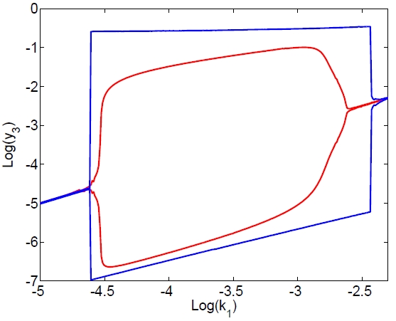
We end this section with a study of the bifurcations of the ODE model and of its tropicalization. It is easy to check that there is only one degree of freedom describing the relative position of the two tropical curves. This is the distance between the origins of the tropical curves, that is given by the combination $k_{1}k_{4}^{\prime-1/2}k_{4}^{1/2}k_{6}^{-1}$. Thus, by changing any one of the parameters $k_{1},k_{4}^{\prime},k_{4},k_{6}$ we can invert the relative position of the tropical curves and change the partition of the logarithmic paper into domains. This leads to two Hopf bifurcations of the ODE model and also two Hopf bifurcations of the tropicalization. The bifurcation of the tropicalization is discontinuous and can also be delayed with respect to the continuous bifurcation of the ODE model (Fig.2).

Figure 2: Hopf bifurcations of the smooth and tropicalized system. (left) The relative positions of the tropical curves can be changed by changing the combination $k_{1}k_{4}^{\prime-1/2}k_{4}^{1/2}k_{6}^{-1}$. The first Hopf bifurcation corresponds to $k_{1}k_{4}^{\prime-1/2}k_{4}^{1/2}k_{6}^{-1}=1$, i.e. $log(k_{1})=-4.61$, when the tropical curves intersect in a single point. For the second Hopf bifurcation the relative position of the two tropical curves is no longer exceptional; the position of the bifurcation results from sliding modes stability analysis. (right) Amplitudes of oscillation are shown for the tropicalization (red) and for the smooth system (blue);

8 Solving ordinary differential equations in triangular form

We give a digest of a general algorithm for solving systems of the type (1) and more generally, an arbitrary system of ordinary differential equations:

$$G_{j}(x_{1},x_{1}^{(1)},\dots,x_{1}^{r},x_{2},x_{2}^{(1)},\dots,x_{2}^{(r)},\dots,x_{n},x_{n}^{(1)},\dots,x_{n}^{(r)},t)=0,\,1\leq j\leq N,$$ (22)

where $G_{j}$ are differential polynomials of the order at most $r$ in the derivatives $x_{i}^{(s)}=\partial^{s}x_{i}/\partial t^{s},\,s\leq r$. Let the degrees of the differential polynomials $G_{j}$ do not exceed $d$. Finally, for algorithmic complexity purposes we assume that the coefficients of $G_{j}$ are integers with absolute values less than $2^{l}$, the latter means that the bit-size of the coefficients $l(G_{j})\leq l$.

In [Sei56] an algorithm was designed which works not only for ordinary differential systems like (22), but even for systems of partial differential equations. For ordinary systems (22) the algorithm was improved in [Gri89], although still its complexity is rather big (see below). We describe the ingredients of the output (which has a triangular form) of the latter improved algorithm and provide for it the complexity bounds.

The algorithm executes the consecutive elimination of the indeterminates $x_{n},\dots,x_{1}$. The algorithm yields a partition $P=\{P_{i}\}_{1\leq i\leq M}$ of the space of the possible functions $x_{1}$. Each $P_{i}$ is given by a system of an equation $f_{i,1}(x_{1},t)=0$ and an inequality $g_{i,1}(x_{1},t)\neq 0$ for suitable differential polynomials $f_{i,1},\,g_{i,1}$. Then the algorithm yields an equation $f_{i,2}(x_{1},x_{2},t)=0$ and an inequality $g_{i,2}(x_{1},x_{2},t)\neq 0$ for $x_{2}$ for suitable differential polynomials $f_{i,2},\,g_{i,2}$. We underline that the latter equation and inequality hold on $P_{i}$. One can treat the system $f_{i,2}=0,\,g_{i,2}\neq 0$ as the conditions on $x_{2}$ with the coefficients being some differential polynomials in $x_{1}$ (satisfying $P_{i}$).

Continuing in a similar way, the algorithm produces a triangular system of differential polynomials $f_{i,3}(x_{1},x_{2},x_{3},t)$, $g_{i,3}(x_{1},x_{2},x_{3},t),\dots$,$f_{i,n}(x_{1},\dots,x_{n},t)$, $g_{i,n}(x_{1},\dots,x_{n},t)$. Thus, at the end $x_{n}$ satisfies (on $P_{i}$) the equation $f_{i,n}(x_{1},\dots,x_{n},t)=0$ and the inequality $g_{i,n}(x_{1},\dots,x_{n},t)\neq 0$ treated as a system with the coefficients being differential polynomials in $x_{1},\dots,x_{n-1}$.

In other words, suppose that one has a device being able to solve an ordinary differential system $f(x)=0,\,g(x)\neq 0$ in a single indeterminate $x$. Then the algorithm would allow one to solve the system (22) consecutively: first producing $x_{1}$ satisfying $f_{i,1}(x_{1},t)=0,\,g_{i,1}(x_{1},t)\neq 0$, after that producing $x_{2}$ satisfying $f_{i,2}(x_{1},x_{2},t)=0,\,g_{i,2}(x_{1},x_{2},t)\neq 0$ and so on.

This completes the description of the output of the algorithm. Now we turn to the issue of its complexity. One can bound the orders of the differential polynomials $ord(f_{i,s}),\,ord(g_{i,s})\leq r\cdot 2^{n}\,:=R,\,1\leq i\leq M,\,1\leq s\leq n$, the number of the elements in the partition and the degrees $M,\,deg(f_{i,s}),\,deg(g_{i,s})\leq(Nd)^{2^{R}}\,:=Q$. Finally, the bit-size of the integer coefficients of $f_{i,s},\,g_{i,s}$ and the complexity of the algorithm can be bounded by a certain polynomial in $l,\,Q$.

Thus, the number $n$ of the indeterminates brings the main contribution into the complexity bound, which is triple exponential in $n$. Of course, the above bounds have an a priori nature: they take into the account all the conceivable possibilities in the worst case, whereas in practical computations considerable simplifications are usually expected.

This illustrates the gain that one can obtain from using tropical geometry to guide model reduction and obtain systems with smaller numbers of indeterminates.

9 Conclusion.

Tropical geometry offers a natural framework to study biochemical networks with multiple timescales and rational reaction rate functions. First, and probably most importantly, tropicalization can guide model reduction of ODE systems. We have shown that the existence of quasi-equilibrium reactions and of quasi-stationary species implies the existence of sliding modes along the tropical variety. Conversely, when the tropicalization has sliding modes along hyperplanes defined by the equality of two monomials, we propose an algorithm to decide whether the system has quasi-equilibrium reactions or quasi-equilibrium species. This distinction allows correct model reduction, and represents an improvement of methods proposed in [RGZL08].

The tropicalization represents an abstraction of the ODE model. This abstraction may be not sound for some dynamic properties, but may conserve others. If the trajectories of the ODE model are either very far or very close to the tropical varieties, they tend to remain close to the trajectories of the tropicalization for a while. However, the quality of the approximation is not guaranteed at finite distance from the tropical variety. For instance, the exit of tropicalized trajectories from a sliding mode tends to be delayed, and smooth trajectories leave earlier neighborhoods of tropical varieties. The example studied in this paper also illustrates some properties of bifurcations of the tropicalization, that we have tested numerically. The tropicalization qualitatively preserves the type and stability of attractors, but can also introduce delays of a Hopf bifurcation. Thus, the tropicalization can only roughly indicate the position of the bifurcation of the ODE model. Furthermore, for Hopf bifurcations, the amplitude of the oscillations behaves differently for the ODE model and for the tropicalization. In fact, Hopf bifurcations are continuous for the ODE model and discontinuous for the tropicalization.

The tropicalization provides in the same time a reduced model and a ”skeleton” for the hybrid dynamics of the reduced model. This skeleton, specified by the tropical varieties, is robust. As a matter of fact, monomials of parameters are generically well separated [GR08]. This implies that tropicalized and smooth trajectories are not that far one from another. Furthermore, because the tropicalized dynamics is robust, it follows that the system can tolerate large relative changes of the parameters without strong modifications of its dynamics.

The dynamics of the model studied in this paper is relatively simple: it has a limit cycle embedded in a two dimensional invariant manifold. As future work we intend to extend the approach to more complex attractors, such as cycles in dimension larger than two and chaotic attractors. Methods to compute tropical varieties in any dimension are well developed in tropical algebraic geometry [BJS⁺07]. Given the tropical variety, the existence of sliding modes can be easily checked and the pruned polynomials defining the fast dynamics calculated. This should lead directly to identification of quasi-equilibrium reactions and quasi-stationary species, without the need of simulation (replaces Step 1 in the Algorithm 1). Proposing simplified descriptions of the dynamics of large and imprecise systems, tropical geometry techniques could find a wide range of applications from synthetic biology design to understanding emerging properties of complex biochemical networks.

Aknowlegments

VN was supported by University of Rennes 1. SV was supported by the Russian Foundation for Basic Research (Grant Nos. 10-01-00627 s and 10-01-00814 a) and the CDRF NIH (Grant No. RR07801) and by a visiting professorship grant from the University of Montpellier 2.

References

- [Aub10] J.P. Aubin. Macroscopic traffic models: Shifting from densities to ”celerities”. Applied Mathematics and Computation, 217:963–971, 2010.
- [BJS+07] T. Bogart, A.N. Jensen, D. Speyer, B. Sturmfels, and R.R. Thomas. Computing tropical varieties. Journal of Symbolic Computation, 42(1-2):54–73, 2007.
- [CDR09] A. Crudu, A. Debussche, and O. Radulescu. Hybrid stochastic simplifications for multiscale gene networks. BMC Systems Biology, 3(1):89, 2009.
- [DFF+07] V. Danos, J. Feret, W. Fontana, R. Harmer, and J. Krivine. Rule-based modelling of cellular signalling. CONCUR 2007–Concurrency Theory, pages 17–41, 2007.
- [FA88] A.F. Filippov and FM Arscott. Differential equations with discontinuous righthand sides, volume 18. Springer, 1988.
- [GR08] AN Gorban and O. Radulescu. Dynamic and static limitation in reaction networks, revisited . In David West Guy B. Marin and Gregory S. Yablonsky, editors, Advances in Chemical Engineering - Mathematics in Chemical Kinetics and Engineering, volume 34 of Advances in Chemical Engineering, pages 103–173. Elsevier, 2008.
- [Gri89] D. Grigoriev. Complexity of quantifier elimination in the theory of ordinary differential equations. Lect. Notes Comput. Sci., 378:11–25, 1989.
- [GRZ10] AN Gorban, O. Radulescu, and AY Zinovyev. Asymptotology of chemical reaction networks. Chemical Engineering Science, 65:2310–2324, 2010.
- [KA56] E.L. King and C. Altman. A schematic method of deriving the rate laws for enzyme-catalyzed reactions. The Journal of Physical Chemistry, 60(10):1375–1378, 1956.
- [LM96] G.L. Litvinov and V.P. Maslov. Idempotent mathematics: a correspondence principle and its applications to computing. Russian Mathematical Surveys, 51(6):1210–1211, 1996.
- [LMS01] G.L. Litvinov, V.P. Maslov, and G.B. Shpiz. Idempotent functional analysis: an algebraic approach. Mathematical Notes, 69(5):696–729, 2001.
- [LY08a] Mark Z. Lazman and Gregory S. Yablonsky. Chapter 2 overall reaction rate equation of single-route complex catalytic reaction in terms of hypergeometric series. In David West Guy B. Marin and Gregory S. Yablonsky, editors, Advances in Chemical Engineering - Mathematics in Chemical Kinetics and Engineering, volume 34 of Advances in Chemical Engineering, pages 47 – 102. Elsevier, 2008.
- [LY08b] M.Z. Lazman and G.S. Yablonsky. Overall reaction rate equation of single-route complex catalytic reaction in terms of hypergeometric series. Advances in Chemical Engineering, 34:47–102, 2008.
- [Mik] G. Mikhalkin. Enumerative tropical algebraic geometry in r2. J. AMS, 18(2):313–377.
- [NVR10] V. Noel, S. Vakulenko, and O. Radulescu. Piecewise smooth hybrid systems as models for networks in molecular biology. In Proceedings of JOBIM 2010. Jobim, 2010.
- [NVR11] V. Noel, S. Vakulenko, and O. Radulescu. Algorithm for identification of piecewise smooth hybrid systems; application to eukaryotic cell cycle regulation. In Proceedings of WABI 2011, to appear, 2011.
- [PS04] L. Pachter and B. Sturmfels. Tropical geometry of statistical models. Proceedings of the National Academy of Sciences of the United States of America, 101(46):16132, 2004.
- [PT05] M. Passare and A. Tsikh. Amoebas: their spines and their contours. In Idempotent mathematics and mathematical physics: international workshop, February 3-10, 2003, Erwin Schrödinger International Institute for Mathematical Physics, Vienna, Austria, volume 377, page 275. Amer Mathematical Society, 2005.
- [RGZL08] O. Radulescu, A.N. Gorban, A. Zinovyev, and A. Lilienbaum. Robust simplifications of multiscale biochemical networks. BMC systems biology, 2(1):86, 2008.
- [Roj03] J.M. Rojas. Why polyhedra matter in non-linear equation solving. In Topics in algebraic geometry and geometric modeling: Workshop on Algebraic Geometry and Geometric Modeling, July 29-August 2, 2002, Vilnius University, Lithuania, volume 334, page 293. Amer Mathematical Society, 2003.
- [Sei56] A. Seidenberg. An elimination theory for differential algebra. Univ. of California Press, 3(2):31–66, 1956.
- [SH10] S. Soliman and M. Heiner. A unique transformation from ordinary differential equations to reaction networks. PloS one, 5(12):e14284, 2010.
- [SS89] L.A. Segel and M. Slemrod. The quasi-steady-state assumption: a case study in perturbation. SIAM Review, 31(3):446–477, 1989.
- [Stu02] B. Sturmfels. Solving systems of polynomial equations. American mathematical society, 2002.
- [TVS85] A. N. Tikhonov, A. B. Vasileva, and A. G. Sveshnikov. Differential equations. Springer, Berlin, 1985.
- [Tys91] J.J. Tyson. Modeling the cell division cycle: cdc2 and cyclin interactions. Proceedings of the National Academy of Sciences of the United States of America, 88(16):7328, 1991.
- [Vir08] O. Viro. From the sixteenth hilbert problem to tropical geometry. Japanese Journal of Mathematics, 3(2):185–214, 2008.
- [Was65] W. Wasow. Asymptotic Expansions for Ordinary Differential Equations. Wiley, New York, 1965.
- [YBGE91] GS Yablonskii, VI Bykov, AN Gorban, and VI Elokhin. Kinetic models of catalytic reactions. Comprehensive Chemical Kinetics, volume 32. Elsevier, Amsterdam, 1991.