Refractive Index of Light in the Quark-Gluon Plasma with the Hard-Thermal-Loop Perturbation Theory

Abstract

The electric permittivity and magnetic permeability for the quark-gluon plasma (QGP) is calculated within the hard-thermal-loop (HTL) perturbation theory. The refractive indices in the magnetizable and nonmagnetizable plasmas are calculated. In a magnetizable plasma, there is a frequency pole $\omega_{mp}$ in the magnetic permeability and the refractive index. The refractive index becomes negative in the range $\omega\in[k,\omega_{mp}]$, where $k$ is the wave number, but no propagating modes are found. In a non-magnetizable plasma, the magnetic permeability and the refractive index are always positive. This marks the main distinction of a weakly coupled plasma from a strongly coupled one, where the negative refraction is shown to exist in a holographic theory.

I Introduction

The quark-gluon plasma (QGP) is believed to be a new state of matter of the strong interaction produced in ultrarelativistic heavy ion collisions (see, e.g., Rischke (2004); Gyulassy and McLerran (2005); Jacobs and Wang (2005); Adams et al. (2005) for reviews). The QGP is a plasma containing electrically charged quarks; its electromagnetic property is an important aspect of its nature. Among all observables for the QGP, the high-energy photons may provide clean probes to hot and dense medium McLerran and Toimela (1985); Kapusta et al. (1991); Alam et al. (2001); Arnold et al. (2001a, b); Adler et al. (2005); Abelev et al. (2010); Prasad (2011). Although the electromagnetic nature gives us an impression that the interaction between low-energy photons and the medium would be weak, it could be more significant than we previously thought due to extremely high temperature and density of the QGP. So the optical properties of the QGP are not a trivial issue.

One of the most important optical properties is the refractive index (RI), which measures the speed of light in a medium relative to vacuum. The negative refraction (NR) is a very interesting phenomenon of materials which was first theoretically proposed by Veselago in 1968 V.G.Veselago (1968). The physical nature of such a property is that the electromagnetic phase velocity is in the opposite direction to the energy flow. The NR leads to many interesting phenomena in materials such as the modified fraction law Shelby et al. (2001); Smith et al. (2004) and bremsstrahlung radiation, the reverse Doppler shift Reed et al. (2003) and Cherenkov radiation, etc.. The most striking application of the NR materials is the optical cloak Schurig et al. (2006), an attractive topic in science fiction. Recently, the strongly coupled plasma has been found to have negative refraction, which was first proposed in Ref. Amariti et al. (2011a) and afterwards followed in Refs. Ge et al. (2011); Gao and Zhang (2010); Bigazzi et al. (2011); Amariti et al. (2011b) in holographic model. Furthermore, it was proven to be a possible generic phenomenon in charged hydrodynamical systems Amariti et al. (2011c).

Motivated by the above finding in the strongly coupled plasma, in this paper we will calculate within the hard-thermal-loop (HTL) perturbation theory the RI via the electric permittivity $\epsilon$ and the magnetic permeability $\mu$. Since a QGP is composed of electrically charged quarks instead of magnetic monopoles, the electric and magnetic sector do not play equal roles. We will show that the physical definition and behavior of $\mu$ (and then the RI) can be very different due to specific magnetic response of the QGP. Therefore a plasma can be classified into two types: magnetizable and nonmagnetizable. In a magnetizable plasma the magnetization is realistic, while in a nonmagnetizable plasma it does not make physical sense any more. We will calculate the RI and analyze their properties in these two types of plasmas. If the QGP is magnetizable, we will show that there is a frequency pole $\omega_{mp}$ in $\mu$ and then the RI, leading to the NRI in the range $\omega\in[k,\omega_{mp}]$, where $k$ is the wave number, but there are no propagating modes in the NRI region. In a nonmagnetizable plasma, $\mu$ and the RI are always positive.

Our results are different from the holographic treatment in following respects. First, in our perturbative treatment with the HTL, the QGP is magnetizable in the frequency range where the NR takes place. The definition of the magnetic permeability is normal and the magnetization density makes physical sense in this region. In contrast, the plasma considered in the holographic theory Amariti et al. (2011a); Ge et al. (2011); Gao and Zhang (2010); Bigazzi et al. (2011); Amariti et al. (2011b) is nonmagnetizable or strongly dielectric, therefore the Landau-Lifshits description L.D.Landau and E.M.Lifshitz (1984) of the magnetic permeability has to be applied. Second, the dispersion relation with the NRI behaves differently. There is a frequency pole below $\omega_{p}$ for $\mu$ and the RI in our approach, but there is no such a singularity in the holographic treatment Amariti et al. (2011a); Ge et al. (2011); Gao and Zhang (2010); Bigazzi et al. (2011); Amariti et al. (2011b). Finally we fail to find any propagating modes with the NRI within the HTL perturbation theory in both magnetizable and nonmagnetizable cases. This marks the main distinction from a strongly coupled plasma where the NR is shown to exist in the holographic theory.

The paper is organized as follows. In Sec. II we briefly review the formalism of computing electromagnetic properties in an isotropic and anisotropy medium. In Sec. III, we calculate the RI from the HTL self-energy of photons in magnetizable and nonmagnetizable plasmas. In Sec. IV, we generalize our calculation to an anisotropic QGP. We finally present the summary and conclusion in Sec. V. We take $k_{B}=\hbar=c=1$ and $g_{\mu\nu}=(+,-,-,-)$ for convention. Here is a summary of abbreviations: quark-gluon plasma (QGP), hard-thermal-loop (HTL), refractive index (RI), negative refraction (NR), negative refraction index (NRI).

II Propagation of electromagnetic wave in medium

The description of electromagnetic waves propagating in a continuous medium is normally given by the electric and magnetic field $E$ and $B$, and the macroscopic field $D$ and $H$. Their relations give the definition of the electric permittivity and the magnetic permeability

$$D_{i} = \epsilon_{ij}(\omega,k)E_{j},$$

$$B_{i} = \mu_{ij}(\omega,k)H_{j},$$ (1)

where $i,j=1,2,3$ are spatial indices, and $\omega$ and $k\equiv|\mathbf{k}|$ are the frequency and wave number, respectively. This scenario applies to magnetizable materials.

Another description was proposed by Landau and Lifshits: that the magnetization $\mathbf{M}$ loses its usual physical meaning as a magnetic moment density, and so does the magnetic permeability $\mu(\omega,k)$, when the characteristic electromagnetic wavelength $\lambda$ is large enough to violate $\lambda^{2}\ll\chi c^{2}/\omega^{2}$, where $\chi$ is the magnetic susceptibility. This scenario applies to nonmagnetizable materials. In this case, $E$, $B$ and $D$ are proper quantities with $\mu(\omega,k)$ being set to unity L.D.Landau and E.M.Lifshitz (1984). The electromagnetic properties of a medium can be provided by

$$D_{i}=\tilde{\epsilon}_{ij}(\omega,k)E_{j},$$ (2)

where $\tilde{\epsilon}(\omega,k)$ is a generalized electric permittivity encoding all electromagnetic response of the medium, in replacement of $\epsilon(\omega,k)$ and $\mu(\omega,k)$ in the conventional case. One can obtain the effective electric permittivity $\epsilon(\omega)$ and magnetic permeability $\mu(\omega)$ by expanding $\tilde{\epsilon}(\omega,k)$ in powers of $k^{2}$ Agranovich et al. (2004)

$$\tilde{\epsilon}(\omega,k) = \epsilon(\omega)+\frac{k^{2}}{\omega^{2}}\left[1-\frac{1}{\mu(\omega)}\right]+\mathcal{O}(k^{4}).$$ (3)

Note that $\epsilon(\omega)$ and $\mu(\omega)$ only depend on $\omega$, and $\mu(\omega)$ comes from the dielectric part of $\tilde{\epsilon}(\omega,k)$ which is different from the conventional definition of the magnetic permeability, especially at low frequency. Only at high frequency, since the magnetic response cannot follow the fast variation of the electromagnetic wave, do these two scenarios coincide and give the vacuum value.

To describe the electromagnetic properties of the QGP covariantly, it is natural to use the fluid four-velocity $u^{\alpha}$ to define the electric and magnetic field strength

$$\tilde{E}^{\mu}=u_{\alpha}F^{\mu\alpha},\;\tilde{B}^{\mu}=\frac{1}{2}\epsilon^{\mu\rho\alpha\beta}u_{\rho}F_{\alpha\beta},$$ (4)

where $\epsilon_{\mu\nu\alpha\beta}=-\epsilon^{\mu\nu\alpha\beta}=-1,1$ for that the order of Lorentz indices $(\mu\nu\alpha\beta)$ is an even/odd permutation of $(0123)$. These quantities are often used when we consider the interaction with a plasma. Then we can immediately write $F^{\mu\nu}$ as

$$F^{\mu\nu}=\tilde{E}^{\mu}u^{\nu}-\tilde{E}^{\nu}u^{\mu}-\epsilon^{\mu\nu\alpha\beta}\tilde{B}_{\alpha}u_{\beta}.$$ (5)

The free action can be expressed in terms of Fourier transformed $\tilde{E}$ and $\tilde{B}$ as

$$S_{0}=-\frac{1}{2}\int\frac{d^{4}K}{(2\pi)^{4}}\left[\tilde{E}^{\mu}(K)\tilde{E}_{\mu}(-K)-\tilde{B}^{\mu}(K)\tilde{B}_{\mu}(-K)\right].$$ (6)

Including the medium effect, the action becomes

$$S = S_{0}-\frac{1}{2}\int\frac{d^{4}K}{(2\pi)^{4}}A^{\mu}(K)\Pi_{\mu\nu}(K)A^{\nu}(-K)+..,$$ (7)

where $A^{\mu}(K)$ is the photon field in momentum space. The medium effect is characterized by the photon self-energy $\Pi_{\mu\nu}(K)$. One can then extract the electric permittivity and the magnetic permeability from the action $S$.

II.1 Isotropic medium

The self-energy must satisfy the Ward identity

$$K^{\mu}\Pi_{\mu\nu}(K)=0,$$ (8)

in which $K_{\mu}=(\omega,k_{i})$ is a 4-momentum. In an isotropic medium, the general solution of Eq.(8) for $\Pi_{\mu\nu}(K)$ is a linear combination of available symmetric tensors

$$\{g_{\mu\nu},\;K_{\mu}K_{\nu},\;u_{\mu}u_{\nu},\;u_{\mu}K_{\nu}+u_{\nu}K_{\mu}\}.$$ (9)

Two independent solutions are the transverse and longitudinal projectors $P_{\mu\nu}$ and $Q_{\mu\nu}$,

$$P_{\mu\nu} = g_{\mu\nu}-u_{\mu}u_{\nu}+\frac{1}{k^{2}}\left(K_{\mu}-\omega u_{\mu}\right)\left(K_{\nu}-\omega u_{\nu}\right),$$

$$Q_{\mu\nu} = \frac{-1}{K^{2}k^{2}}\left(\omega K_{\mu}-K^{2}u_{\mu}\right)\left(\omega K_{\nu}-K^{2}u_{\nu}\right).$$ (10)

Therefore $\Pi_{\mu\nu}(K)$ can be expanded in these projectors as

$$\Pi_{\mu\nu}(K)=\Pi_{T}(K)P_{\mu\nu}+\Pi_{L}(K)Q_{\mu\nu},$$ (11)

where $\Pi_{T/L}(K)$ are transverse/longitudinal part of the self-energy. The full inverse propagator for the photon is

$$D_{\mu\nu}^{-1} = D_{(0)\mu\nu}^{-1}+\Pi_{\mu\nu}=(-K^{2}+\Pi_{L})Q_{\mu\nu}+(-K^{2}+\Pi_{T})P_{\mu\nu}-\frac{1}{1-\eta}K_{\mu}K_{\nu}$$ (12)

where the last term is the gauge-fixing term and $\eta$ is the gauge parameter. Here we choose the covariant gauge $K\cdot A_{K}=0$ so the gauge-fixing term does not appear in the action.

In magnetizable case, the action can then be evaluated with $D_{\mu\nu}^{-1}(K)$ as

$$S = \frac{1}{2}\int d^{4}KA_{\mu}(K)\left(D^{-1}\right)^{\mu\nu}A_{\nu}(-K)$$ (13)

$$= -\frac{1}{2}\int d^{4}K\left[\epsilon_{\mu\nu}\tilde{E}^{\mu}(K)\tilde{E}^{\nu}(-K)-\frac{1}{\mu}\tilde{B}_{\mu}(K)\tilde{B}^{\mu}(-K)\right],$$

where

$$\epsilon_{\mu\nu}(\omega,k) = \epsilon(\omega,k)g_{\mu\nu}=\left(1-\frac{\Pi_{L}}{K^{2}}\right)g_{\mu\nu},$$

$$\frac{1}{\mu(\omega,k)} = 1+\frac{K^{2}\Pi_{T}-\omega^{2}\Pi_{L}}{k^{2}K^{2}}.$$ (14)

In the nonmagnetizable case or the Landau-Lifshits scenario, we obtain

$$S=-\frac{1}{2}\int d^{4}K\left[\tilde{\epsilon}\tilde{E}_{\mu}(K)\tilde{E}^{\mu}(-K)-\tilde{B}_{\mu}(K)\tilde{B}^{\mu}(-K)\right],$$ (15)

where

$$\tilde{\epsilon}(\omega,k)=1-\frac{\Pi_{T}}{\omega^{2}}.$$ (16)

Then the effective electric permittivity and magnetic permeability can be extracted from $\tilde{\epsilon}(\omega,k)$

$$\epsilon(\omega) = 1-\frac{\Pi_{T}^{(0)}(\omega)}{\omega^{2}},$$

$$\frac{1}{\mu(\omega)} = 1+\Pi_{T}^{(2)}(\omega),$$ (17)

where we have expanded the $\Pi_{T}$ in powers of $k$ by

$$\Pi_{T}(\omega,k)=\Pi_{T}^{(0)}(\omega)+k^{2}\Pi_{T}^{(2)}(\omega)+\mathcal{O}(k^{4}).$$ (18)

II.2 Anisotropic medium

Suppose there is one special direction $r_{\mu}=(0,\mathbf{r})$ in a most simple anisotropic medium. Now there are three vectors $\{\tilde{r}_{\mu},K_{\mu},u_{\mu}\}$ out of which the tensorial bases for $\Pi_{\mu\nu}$ are composed, where $\tilde{r}_{\mu}\equiv P_{\mu\nu}r^{\nu}$ is a vector normal to $K^{\mu}$ with $P_{\mu\nu}$ defined by Eq. (10). The available symmetric tensors have additional elements besides those in (9),

$$\{...,\;\tilde{r}_{\mu}\tilde{r}_{\nu},\;\tilde{r}_{\mu}K_{\nu}+\tilde{r}_{\nu}K_{\mu},\;\tilde{r}_{\mu}u_{\nu}+\tilde{r}_{\nu}u_{\mu}\}.$$ (19)

As a consequence, the tensorial bases that satisfy the Ward identity (8) now become

$$\{P_{\mu\nu},Q_{\mu\nu},C_{\mu\nu},G_{\mu\nu}\},$$ (20)

where two extra projectors are given by

$$C_{\mu\nu} = \frac{\tilde{r}_{\mu}\tilde{r}_{\nu}}{\tilde{r}^{2}},$$

$$G_{\mu\nu} = \left(K_{\mu}\tilde{r}_{\nu}+K_{\nu}\tilde{r}_{\mu}\right)-\frac{K^{2}}{\omega}\left(\tilde{r}_{\mu}u_{\nu}+\tilde{r}_{\nu}u_{\mu}\right),$$ (21)

which obey $K^{\mu}C_{\mu\nu}=K^{\mu}G_{\mu\nu}=0$. Then the self-energy tensor can be expanded as

$$\Pi_{\mu\nu}=\alpha P_{\mu\nu}+\beta Q_{\mu\nu}+\gamma C_{\mu\nu}+\delta G_{\mu\nu},$$ (22)

where $\alpha,\beta,\gamma,\delta$ are structure functions. Inserting the above into the full propagator inverse $D_{\mu\nu}^{-1}(K)$ one obtains the full action (13) with

$$\epsilon_{\mu\nu} = \left(1-\frac{\beta}{K^{2}}\right)g_{\mu\nu}-\frac{1}{\omega^{2}}\left[\gamma\frac{\tilde{r}_{\mu}\tilde{r}_{\nu}}{\tilde{r}^{2}}+\delta\left(K_{\mu}\tilde{r}_{\nu}+K_{\nu}\tilde{r}_{\mu}\right)\right],$$

$$\frac{1}{\mu} = 1+\frac{K^{2}\alpha-\omega^{2}\beta}{k^{2}K^{2}}.$$ (23)

The transverse component of the action (13) gives

$$S_{T} = -\frac{1}{2}\int d^{4}K\left[\epsilon_{\mu\nu}^{T}\tilde{E}_{T}^{\mu}(K)\tilde{E_{T}^{\nu}}(-K)-\frac{1}{\mu}\tilde{B}_{\mu}(K)\tilde{B}^{\mu}(-K)\right],$$ (24)

where $\tilde{E}_{T}^{\mu}(K)=P^{\mu\nu}\tilde{E}_{T,\nu}(K)$. Note that the magnetic part is always transverse. $\epsilon_{\mu\nu}^{T}$ is the transverse projection of $\epsilon_{\mu\nu}$ and is given by

$$\epsilon_{\mu\nu}^{T} = \left(1-\frac{\beta}{K^{2}}\right)g_{\mu\nu}-\frac{\gamma}{\omega^{2}}C_{\mu\nu},$$ (25)

Similarly, in the nonmagnetizable case, the transverse part of the action is

$$S_{T}=-\frac{1}{2}\int d^{4}K\left[\tilde{\epsilon}_{\mu\nu}^{T}\tilde{E}_{T}^{\mu}(K)\tilde{E}_{T}^{\nu}(-K)-\tilde{B}_{\mu}(K)\tilde{B}^{\mu}(-K)\right],$$ (26)

where

$$\tilde{\epsilon}_{\mu\nu}^{T}=\left(1-\frac{\alpha}{\omega^{2}}\right)g_{\mu\nu}-\frac{\gamma}{\omega^{2}}C_{\mu\nu}.$$ (27)

One has to diagonalize $\epsilon_{\mu\nu}^{T}$ (magnetizable case) and $\tilde{\epsilon}_{\mu\nu}^{T}$ (nonmagnetizable case) in order to obtain the eigenvalues of the electric permittivity for the left- and right-handed polarized photons. Let us consider an analytically solvable case as follows. In a rest frame with the fluid velocity $u^{\mu}=(1,0,0,0)$, since $\tilde{E}^{0}=0$, so the spatial part of $\epsilon_{\mu\nu}^{T}$ or $\tilde{\epsilon}_{\mu\nu}^{T}$, a $3\times 3$ matrix $\epsilon_{ij}^{T}$ or $\tilde{\epsilon}_{ij}^{T}$ for $i,j=1,2,3$, is

$$\epsilon_{ij}^{T}=\left(1-\frac{\beta}{K^{2}}\right)\delta_{ij}-\frac{\gamma}{\omega^{2}}\frac{\mathbf{r}_{Ti}\mathbf{r}_{Tj}}{\mathbf{r}_{T}^{2}},$$

and

$$\tilde{\epsilon}_{ij}^{T}=\left(1-\frac{\alpha}{\omega^{2}}\right)\delta_{ij}-\frac{\gamma}{\omega^{2}}\frac{\mathbf{r}_{Ti}\mathbf{r}_{Tj}}{\mathbf{r}_{T}^{2}},$$

where we have defined $\mathbf{r}_{T}=\mathbf{r}-(\mathbf{r}\cdot\hat{\mathbf{k}})\hat{\mathbf{k}}$ and used $\tilde{r}^{2}=-\tilde{\mathbf{r}}_{T}^{2}$. One obtains the eigenvalues for the left- and right-handed polarized photons, for a magnetizable plasma,

$$\epsilon_{L}=1-\frac{\beta}{K^{2}},\;\epsilon_{R}=1-\frac{\beta}{K^{2}}-\frac{\gamma}{\omega^{2}},$$ (28)

and those for an nonmagnetizable plasma,

$$\tilde{\epsilon}_{L}=1-\frac{\alpha}{\omega^{2}},\;\tilde{\epsilon}_{R}=1-\frac{\alpha}{\omega^{2}}-\frac{\gamma}{\omega^{2}}.$$ (29)

II.3 Refractive Index

The refractive index is normally defined by $n^{2}=\epsilon\mu$, but the quadratic nature of such a definition implies that it is not sensitive to the sign of $\epsilon$ and $\mu$. It is known that the sign change of $\epsilon$ and $\mu$ corresponds to a cross over between different branches of the square root, from $n=\sqrt{\epsilon\mu}$ to $n=-\sqrt{\epsilon\mu}$, or from the positive refractive index to the negative one. We can see in the following that the sign of $\epsilon$ and $\mu$ have a significant physical implication. The phase velocity is defined by

$$\mathbf{v}_{p}=\frac{1}{\mathrm{Re}(n)}\hat{\mathbf{k}}=v_{p}\hat{\mathbf{k}},$$ (30)

whose sign is the same as that of $\mathrm{Re}(n)$. But the direction of the energy flow or the Poynting vector is not affected by the sign of $\epsilon$ and $\mu$. In a medium with small dissipation, the direction of the energy flow coincides with that of the group velocity,

$$\mathbf{S}=v_{g}U\hat{\mathbf{k}},$$ (31)

where $U$ is a positive time-averaged energy density and $v_{g}=d\omega/dk$.

So the direction of the phase velocity can be opposite to the energy flow or the group velocity if we have, e.g., a negative phase velocity and a positive group one or vice versa

$$v_{p}<0,\;v_{g}>0.$$ (32)

This criterion of the antiparallelism for the phase velocity and the energy flow is equivalent to a better definition called the Depine-Lakhtakia (DL) index R.A.Depine and A.Lakhtakia (2004),

$$n_{DL}=\left|\epsilon\right|\mathrm{Re}(\mu)+\left|\mu\right|\mathrm{Re}(\epsilon).$$ (33)

When $n_{DL}<0$, the directions of the phase velocity and the energy flow are opposite. So $n_{DL}$ is a good quantity for covering the NRI. We will calculate both $n_{DL}$ and $n$ in the next section.

III Hard-Thermal-Loop self-energy for photon

The self-energy tensor of photon in a plasma can be calculated by the standard perturbative technique of Feynman diagram at finite temperature and density (i.e., a finite chemical potential). However, a complete calculation of $\Pi_{\mu\nu}$ is rather involved because of the significantly high temperature of the QGP, even at one loop level in which the self-energy is given by the exchange of quark loops, so we only limit ourselves to the high-temperature approximation, which means that the temperature is much larger than the quark mass and external momenta, named the HTL part of $\Pi_{\mu\nu}$. In this section, we will investigate the refractive index for the HTL self-energy $\Pi_{\mu\nu}$ of the photon from the quark loops in the QGP Weldon (1982); Pisarski (1989); Bellac (1996). The HTL approximation works well at high temperature where the QGP is thought to be weakly coupled. The HTL self-energy reads

$$\Pi_{T}(\omega,k) = \frac{1}{2}m_{D}^{2}\left[\frac{\omega^{2}}{k^{2}}+\left(1-\frac{\omega^{2}}{k^{2}}\right)\frac{\omega}{2k}\log\frac{\omega+k}{\omega-k}\right],$$

$$\Pi_{L}(\omega,k) = m_{D}^{2}\left(1-\frac{\omega^{2}}{k^{2}}\right)\left[1-\frac{\omega}{2k}\log\frac{\omega+k}{\omega-k}\right],$$ (34)

in which the Debye mass squared is

$$m_{D}^{2}\equiv e^{2}N_{c}\sum^{N_{f}}_{f}\left(\frac{1}{3}T^{2}+\frac{\mu_{f}^{2}}{\pi^{2}}\right)Q_{f}^{2},$$ (35)

where $e$ is the electric charge, $\mu_{f}$ and $Q_{f}$ are the quark chemical potential and the electric charge for the flavor species $f$, $N_{c}$ and $N_{f}$ are the number of colors and flavors, respectively. When $\omega>k$, $\Pi_{T,L}(\omega,k)$ are real, meaning that the medium has no dissipation for propagating modes. When $k>\omega$, the imaginary parts appear, the medium becomes dissipative due to the Landau damping effect.

III.1 Magnetizable Plasma

A magnetizable plasma is the one in which the magnetic moment and the magnetic permeability $\mu(\omega,k)$ have ordinary physical meanings. Substituting the self-energy (34) into Eq. (14) we obtain

$$\epsilon(\omega,k) = 1+\frac{m_{D}^{2}}{k^{2}}\left(1-\frac{\omega}{2k}\log\frac{\omega+k}{\omega-k}\right),$$

$$\mu(\omega,k) = \frac{4k^{4}}{4k^{4}+6m_{D}^{2}\omega^{2}+m_{D}^{2}(k^{2}-3\omega^{2})\frac{\omega}{k}\log\frac{\omega+k}{\omega-k}}.$$ (36)

In principle, the plasma contains not only temporal dispersion, but also spatial dispersion. In an isotropic medium, if the phase velocity of light is much larger than the thermal velocity of plasma particles, the spatial dispersion is small, and then $\epsilon(\omega,k)$ and $\mu(\omega,k)$ can be assumed to be independent of $k$. In this small $k$ limit, we have $\omega>k$, both $\epsilon(\omega,k)$ and $\mu(\omega,k)$ are real. This is equivalent to expanding $\epsilon(\omega,k)$ and $\mu(\omega,k)$ in $k$ around $k=0$

$$\epsilon(\omega) \approx 1-\frac{m_{D}^{2}}{3\omega^{2}}+\mathcal{O}(k^{2}),$$

$$\mu(\omega) \approx \frac{1}{1-\frac{2m_{D}^{2}}{15\omega^{2}}}+\mathcal{O}(k^{2}).$$ (37)

The first observation of Eq. (37) is that $\epsilon(\omega)$ is negative for $\omega<\omega_{p}=\sqrt{1/3}m_{D}$, where $\omega_{p}$ is called the Debye screening frequency. The second observation is: there is a pole at $\omega_{mp}=\sqrt{2/15}m_{D}$ in $\mu(\omega)$, below which both $\epsilon(\omega)$ and $\mu(\omega)$ become negative. We show $n^{2}$ and $n_{DL}$ as functions of $\omega/m_{D}$ in Fig. 1. At high frequencies, the refractive index is always less than unity, meaning that the phase velocity is greater than the speed of light. There is a frequency gap between $\omega_{mp}$ and $\omega_{p}$ where $n^{2}<0$ and $n_{DL}=0$. For frequencies in the gap, the light cannot propagate or the plasma is opaque to electromagnetic waves. The width of the gap is proportional to $m_{D}$, i.e., the higher the temperatures and/or densities, the broader the gap is. At frequencies lower than the pole, $k<\omega<\omega_{mp}$, $n_{DL}$ becomes negative. However, the propagating modes should satisfy the transverse dispersion relation $n^{2}\omega^{2}=k^{2}$; it has no solution in the range $\omega\in[k,\omega_{mp}]$, indicating that there are no propagating modes in the NRI region. Note that $\mu(\omega)$ and $n^{2}$ diverge at $\omega_{mp}$, where the magnetization is large and resonantly oscillates with the electromagnetic wave. The phase and group velocity are small in the region and approaches zero at $\omega_{mp}$. In the range $\omega\in[\omega_{mp},\omega_{p}]$, we see $n^{2}<0$, i.e., the RI is purely imaginary and the electromagnetic wave is damped.

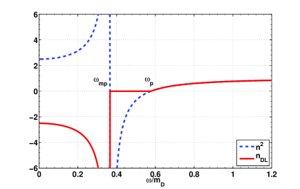
Figure 1: The RI for a magnetizable plasma in small $k$ expansion: the conventional refractive index $n^{2}$ and the Depine-Lakhtakia index $n_{DL}$ as functions of $\omega$. We take $m_{D}$ as the unit for $k$ and $\omega$.

Now we can go beyond the small $k$ limit by working with the full version of $\epsilon$ and $\mu$ in Eq. (36). We show $n$ and $n_{DL}$ at a fixed value $k/m_{D}=0.2$ in Fig. 2. The values of $\omega_{mp}$ and $\omega_{p}$ increases with $k$. There is a jump in $n_{DL}$ and $\mathrm{Re}(n)$ at $\omega=k$, they change from positive to negative values from $\omega<k$ to $\omega>k$. When $\omega<k$, both $\epsilon$ and $\mu$ become complex, indicating that the medium is dissipative. When $k<\omega<\omega_{mp}$, we have $n_{DL}<0$ and $\mathrm{Re}(n)<0$, but no propagating modes are found since the dispersion $n^{2}\omega^{2}=k^{2}$ cannot hold in this region. In the frequency range, $\omega_{mp}<\omega<\omega_{p}$, the refractive index is purely imaginary, so any propagating modes are forbidden. When $\omega_{p}<\omega$, there are normal propagating modes with positive refraction. The dispersion relation $\omega(k)$ is shown in Fig. 3.

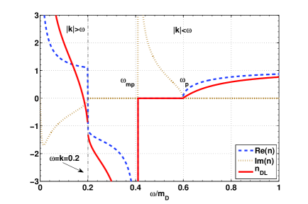
Figure 2: The refractive indices $n$ (real part: blue dashed, imaginary part: brown dotted) and $n_{DL}$ (red solid) for a magnetizable plasma at $k=0.2$. In the region $\omega<k=0.2$, $n$ is complex and has real and imaginary parts, meaning that the medium is dissipative. In the range $k<\omega<\omega_{mp}$, $n$ is purely real and negative, $n<0$, but there is no propagating mode which satisfies the dispersion $n^{2}\omega^{2}=k^{2}$. In the range $\omega_{mp}<\omega<\omega_{p}$, $n$ becomes purely imaginary, so the medium is opaque. When $\omega_{p}<\omega$, the real part of $n$ is positive, $\mathrm{Re}(n)>0$. We take $m_{D}$ as the unit for $k$ and $\omega$.

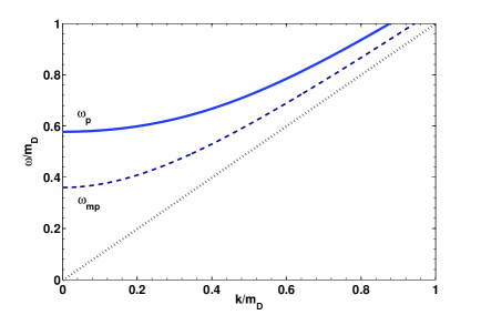
Figure 3: The dispersion relation $\omega(k)$ for magnetizable and nonmagnetizable plasmas (blue solid line). The dotted line is the light cone $\omega=k$. If the plasma is magnetizable, we have poles on the dashed line, but there are no poles in nonmagnetizable plasma. We take $m_{D}$ as the unit for $k$ and $\omega$.

III.2 Nonmagnetizable plasma

However, a completely different situation appears in a nonmagnetizable plasma. At high enough frequencies, or if the magnetic susceptibility $\chi$ is small and the plasma has a long relaxation time, the magnetic moments of particles in the plasma cannot respond to the time variation of an electromagnetic wave in time. In this case, as was argued by Landau and Lifshits, the magnetization loses its physical meaning, and we need to treat this problem in an alternative approach by taking the magnetic permeability to the vacuum value, $\mu=1$. Then the effective permeability comes from the spatial part of the generalized permittivity $\tilde{\epsilon}$. By expanding $\Pi_{T}(\omega,k)$ in powers of $k$ at $k=0$

$$\Pi_{T}(\omega,k)=m_{D}^{2}\left(\frac{1}{3}+\frac{1}{15}\frac{k^{2}}{\omega^{2}}\right)+\mathcal{O}(k^{4}),$$ (38)

we then obtain from Eq. (17),

$$\epsilon(\omega) = 1-\frac{m_{D}^{2}}{3\omega^{2}},\;\mu(\omega)=\frac{1}{1+\frac{m_{D}^{2}}{15\omega^{2}}}.$$ (39)

It is obvious that $\epsilon$ is the same as in the magnetizable case. But the effective magnetic permeability $\mu$ is always positive, so the NRI is absent. A complete screening gap up to $\omega_{p}$ is present, only the mode with frequencies higher than $\omega_{p}$ can propagate. The dispersion relation is the same as the Fig. 3, but $n$ below the plasma frequency is purely imaginary ($n^{2}<0$) and hence all modes are damped, see Fig. 4.

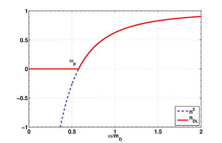
Figure 4: The RI for the nonmagnetizable plasma by the conventional refractive index $n^{2}$ and the Depine-Lakhtakia index $n_{DL}$ as functions of $\omega$. We take $m_{D}$ as the unit for $k$ and $\omega$.

III.3 A criterion for magnetizable and nonmagnetizable plasma

As we can see from the above discussions, the magnetic response is essential in justification of the QGP as a magnetizable or nonmagnetizable medium. The core question is then: whether the magnetization density has physical meaning for the plasma. To this end we look at the induced macroscopic current density $\mathbf{J}$ from not only the magnetization $\mathbf{M}=(\mathbf{B}-\mathbf{H})/4\pi$ but also the dielectric polarization $\mathbf{P}=(\mathbf{D}-\mathbf{E})/4\pi$,

$$\mathbf{J}=\nabla\times\mathbf{M}+\frac{\partial\mathbf{P}}{\partial t},$$ (40)

which can be derived directly from the Maxwell equations

$$\nabla\times\mathbf{B} = \mathbf{J}+\frac{\partial\mathbf{E}}{\partial t},$$

$$\nabla\times\mathbf{H} = \frac{\partial\mathbf{D}}{\partial t}.$$ (41)

We can compare the contribution from the electric and magnetic sector to the induced current and see if the concept of the magnetization still works. When the current is dominated by the magnetization, the following condition must be satisfied

$$\left|\nabla\times\mathbf{M}\right|\gg\left|\frac{\partial\mathbf{P}}{\partial t}\right|,$$ (42)

which is equivalent to

$$R(\omega)=\left|\frac{\epsilon(\omega)\left(\mu(\omega)-1\right)}{\epsilon(\omega)-1}\right|\gg 1.$$ (43)

We can use Eqs. (36,37) to test if $R(\omega)\gg 1$ holds or not. If it does, the magnetization density makes a dominant contribution to the induced current density, so the plasma is magnetizable and Eqs. (36,37) apply. If this condition is violated, the magnetization density is negligible and the plasma is an nonmagnetizable medium. In this case, $\mu(\omega)$ in Eqs. (36,37) loses its normal meaning and is not applicable. Thus one has to implement the Landau-Lifshits scenario. Therefore, Eq. (43) can be regarded as a criterion to judge if a plasma is magnetizable or nonmagnetizable.

In our study, as shown in Fig. 5, the criterion (43) is valid near the pole $\omega_{mp}$, below which the refractive index becomes negative. So near the pole $\omega_{mp}$ the plasma is magnetizable, otherwise it is nonmagnetizable.

Although the dispersion relation shown in Fig. 3 seems to be the same in magnetizable and nonmagnetizable plasmas, completely different behaviors of the RI occur below $\omega_{p}$. The main difference is the existence of a pole in the magnetizable plasma corresponding to a resonance. In this region, the phase velocity is slowed down and vanishing at the pole, so the thermal velocity is much greater than the phase velocity and the plasma becomes strongly anisotropic, which is beyond the scope of this paper.

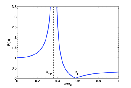
Figure 5: The ratio $R(\omega)$ as a function of $\omega$ for a fixed and small value of $k$. $R(\omega)\gg 1$ is valid in the range $\omega\lesssim\omega_{mp}$ where the refractive index becomes negative.

Our approach is based on the HTL perturbation, which is quite different from the holographic approach. The dispersion relation behaves differently in two approaches. In our approach there is a frequency range with $n^{2}<0$ corresponding to a forbidden band for electromagnetic waves in between the negative and positive refraction region, while in the holographic theory the dispersion relation is continuous. This distinction is closely related to the effectiveness of the notion of quasiparticles. In addition, there is a pole at $\omega_{mp}$ in the HTL approach which makes $n^{2}$ and $n_{DL}$ singular. Such a property is possibly a feature for the magnetizable plasma in a weakly coupled system. In contrast, in the holographic theory for the nonmagnetizable and strongly coupled plasma, there is no such a pole.

IV Anisotropic quark matter

In Sec. III we have considered an isotropic quark matter. The quark momentum distribution is anisotropic at early time in noncentral heavy ion collisions. A proper way of generalizing to an anisotropic case is to derive the self-energy using the kinetic theory. Here we consider the quark distribution function $f_{a}(p)$ for $a=u,d,s,\bar{u},\bar{d},\bar{s}$, which obey the Boltzmann equation; the self-energy can be expressed by $f_{a}(p)$ Romatschke and Strickland (2003, 2004)

$$\Pi_{\mu\nu}(K)=-2e^{2}N_{c}\sum_{a}Q_{a}^{2}\int\frac{d^{3}p}{(2\pi)^{3}}V_{\mu}\frac{\partial f_{a}(p)}{\partial P_{i}}\left(g_{\nu i}-\frac{V_{\nu}K_{i}}{K\cdot V+i\eta}\right)$$ (44)

where the four-velocity is defined by $V^{\mu}=P^{\mu}/p=(1,\mathbf{v})=(1,\mathbf{p}/p)$ and $f_{a}(p)=1/(e^{\beta p-\beta\mu_{a}}+1)$. Here the summation for $i$ is over spatial components. Note that $\Pi_{\mu\nu}(K)$ has a different sign in our convention from Refs. Romatschke and Strickland (2003, 2004). To generalize Eq. (44) to anisotropic case, we can make replacement in distribution function $f(p)$

$$p\rightarrow\tilde{p}=\left[p^{2}+\xi(\mathbf{p}\cdot\mathbf{r})^{2}\right]^{1/2},$$ (45)

where $\xi$ parametrizes the strength of the anisotropy: a positive/negative value of $\xi$ corresponds to a contraction/stretching of the isotropic distribution function along $\mathbf{r}$. Then the self-energy becomes

$$\Pi_{\mu\nu}(K) = -2e^{2}N_{c}\sum_{a}Q_{a}^{2}\int\frac{d^{3}p}{(2\pi)^{3}}V_{\mu}\frac{\partial f_{a}(\tilde{p})}{\partial P_{i}}\left(g_{\nu i}-\frac{V_{\nu}K_{i}}{K\cdot V+i\eta}\right)$$ (46)

$$= -m_{D}^{2}\int\frac{d\Omega}{4\pi}\frac{\mathbf{v}_{i}+\xi(\mathbf{v}\cdot\mathbf{r})\mathbf{r}_{i}}{[1+\xi(\mathbf{v}\cdot\mathbf{r})^{2}]^{2}}V_{\mu}\left(g_{\nu i}-\frac{V_{\nu}K_{i}}{K\cdot V+i\eta}\right).$$

The spatial component $\Pi_{ij}$ is then

$$\Pi_{jl} = -m_{D}^{2}\int\frac{d\Omega}{4\pi}\frac{\mathbf{v}_{i}+\xi(\mathbf{v}\cdot\mathbf{r})\mathbf{r}_{i}}{[1+\xi(\mathbf{v}\cdot\mathbf{r})^{2}]^{2}}\mathbf{v}_{j}\left(\delta_{li}+\frac{\mathbf{v}_{l}\mathbf{k}_{i}}{K\cdot V+i\eta}\right).$$ (47)

The four structure functions in Eq. (22) can be extracted by the following contractions:

$$\alpha = (P_{\mu\nu}-C_{\mu\nu})\Pi^{\mu\nu},$$

$$\beta = Q_{\mu\nu}\Pi^{\mu\nu},$$

$$\gamma = (2C_{\mu\nu}-P_{\mu\nu})\Pi^{\mu\nu},$$

$$\delta = -\frac{1}{2}\frac{\omega^{2}}{K^{2}k^{2}\tilde{r}^{2}}G_{\mu\nu}\Pi^{\mu\nu}.$$ (48)

We assume that the magnitude of the anisotropy is small so that we can perform an expansion in powers of $\xi$ for $\Pi_{jl}$,

$$\Pi_{jl}(K) = \Pi_{jl}^{(HTL)}(K)+\xi m_{D}^{2}\int\frac{d\Omega}{4\pi}[(\mathbf{v}\cdot\mathbf{r})\mathbf{r}_{i}-2(\mathbf{v}\cdot\mathbf{r})^{2}\mathbf{v}_{i}]\mathbf{v}_{j}$$ (49)

$$\times\left(\delta_{li}+\frac{\mathbf{v}_{l}\mathbf{k}_{i}}{K\cdot V+i\eta}\right)+O(\xi^{2}),$$

where the HTL self-energy is given by,

$$\Pi_{jl}^{(HTL)}(K)=-m_{D}^{2}k_{0}\int\frac{d\Omega}{4\pi}\frac{\mathbf{v}_{j}\mathbf{v}_{l}}{k_{0}-\mathbf{v}\cdot\mathbf{k}+i\eta}.$$ (50)

Up to $O(\xi)$ the structure functions relevant to the refractive index of transverse modes can be obtained,

$$\alpha = \Pi_{T}(z)+\xi\left\{\frac{z^{2}}{12}\left(3+5\cos 2\theta\right)m_{D}^{2}-\frac{1}{6}\left(1+\cos 2\theta\right)m_{D}^{2}\right.$$ (51)

$$\left.+\frac{1}{4}\Pi_{T}(z)\left[(1+3\cos 2\theta)-z^{2}(3+5\cos 2\theta)\right]\right\},$$

$$\beta = \Pi_{L}(z)+\xi\biggl{\{}\frac{1}{6}(z^{2}-1)(1+3\cos 2\theta)m_{D}^{2}+\Pi_{L}(z)$$ (52)

$$\times\left(\cos 2\theta-\frac{z^{2}}{2}(1+3\cos 2\theta)\right)\biggr{\}},$$

$$\gamma = \frac{\xi}{3}[3\Pi_{T}(z)-m_{D}^{2}](z^{2}-1)\sin^{2}\theta,$$ (53)

where $\Pi_{T}(z)$ and $\Pi_{L}(z)$ is the standard HTL result in Eq. (34), $z=\omega/k$, and $\theta$ is the angle between the direction of the wave vector of the light and the anisotropy, $\cos\theta=\mathbf{\mathbf{k}}\cdot\mathbf{r}$. In the limit $\xi\rightarrow 0$, the above structure functions $\alpha$ and $\beta$ reduce to the isotropic HTL case, while $\gamma$ and $\delta$ vanish.

First, we focus on the magnetizable case. We diagonalize $\epsilon_{ij}$ in Eq.(28) in the plane perpendicular to $\mathbf{k}$, in small $k$ approximation, we get

$$\epsilon_{L}^{(mag)}(\omega) = 1-\frac{m_{D}^{2}}{3\omega^{2}}+\xi\frac{m_{D}^{2}}{10\omega^{2}}\left(1-\frac{1}{3}\cos 2\theta\right)+\mathcal{O}(k^{2},\xi),$$ (54)

$$\epsilon_{R}^{(mag)}(\omega) = 1-\frac{m_{D}^{2}}{3\omega^{2}}+\xi\frac{m_{D}^{2}}{15\omega^{2}}+\mathcal{O}(k^{2},\xi).$$ (55)

However, in an anisotropic medium, the spatial dispersion becomes important, as one can see in the following that the term with $k$ is always accompanied by $\xi$, so small $k$ expansion has to be treated with more care. We have assumed $\xi\ll 1$ and $k\ll 1$, if we further assume $\xi/k^{2}$ is small compared with the leading term $1-\frac{2m_{D}^{2}}{15\omega^{2}}$, the expansion can lead to

$$\mu^{(mag)}(\omega,k)=\frac{1}{1-\frac{2m_{D}^{2}}{15\omega^{2}}-\xi\frac{m_{D}^{2}}{15k^{2}}\cos^{2}\theta+\mathcal{O}(k^{2},\xi)}.$$ (56)

If the ratio $\xi/k^{2}$ is not small, it becomes a singular term of $\mathcal{O}(1/k^{2})$, the expansion in small $k$ fails, and a more rigorous consideration is required by solving the full version of the dispersion relation. In the nonmagnetizable case, we have

$$\epsilon_{L}^{(non)}(\omega) =1-\frac{m_{D}^{2}}{3\omega^{2}}+\xi\frac{2m_{D}^{2}}{15\omega^{2}},$$ (57)

$$\epsilon_{R}^{(non)}(\omega) =1-\frac{m_{D}^{2}}{3\omega^{2}}+\xi\frac{m_{D}^{2}}{10\omega^{2}}\left(1+\frac{1}{3}\cos 2\theta\right),$$ (58)

and

$$\mu_{L}^{(non)}(\omega) =\frac{1}{1+\frac{m_{D}^{2}}{15\omega^{2}}-\xi\frac{m_{D}^{2}}{70\omega^{2}}\left(\frac{1}{3}-\cos 2\theta\right)},$$ (59)

$$\mu_{R}^{(non)}(\omega) =\frac{1}{1+\frac{m_{D}^{2}}{15\omega^{2}}-\xi\frac{m_{D}^{2}}{6\omega^{2}}\left(\frac{1}{7}-\frac{1}{5}\cos 2\theta\right)}.$$ (60)

In this section, the anisotropy is just a small correction to the isotropic result, the plasma frequency $\omega_{p}$ and pole $\omega_{mp}$ change a little by extra parameters $\xi$ and $\theta$ introduced from anisotropy.

V Summary and conclusion

We study the electromagnetic wave properties of the QGP within the HTL perturbation theory. The electric permittivity, the magnetic permeability and then the optical refractive index are calculated in magnetizable and nonmagnetizable plasmas. The optical properties of these two types of plasmas behave differently at low frequencies due to different definitions of the magnetic permeability $\mu$. The plasma is magnetizable if $R(\omega)=\left|\frac{\epsilon(\omega)\left(\mu(\omega)-1\right)}{\epsilon(\omega)-1}\right|\gg 1$, while it is nonmagnetizable if this condition does not hold.

In the magnetizable plasma, $\mu$ has the normal physical meaning, but it fails to make physical sense in the nonmagnetizable plasma. In the magnetizable plasma, $\mu$ has a pole at $\omega_{mp}$ below the plasma frequency $\omega_{p}$. When $k<\omega<\omega_{mp}$, both $n$ and $n_{DL}$ become negative but no propagating modes exist. A frequency forbidden band or a gap with imaginary $n$ or $n^{2}<0$ is in the range $\omega_{mp}<\omega<\omega_{p}$, where electromagnetic waves are damped. For $\omega<k$, $n$ becomes complex and the medium is dissipative. In the nonmagnetizable plasma, both $\mu$ and $n_{DL}$ are non-negative. The damped region or the gap is in the range $\omega<\omega_{p}$.

In contrast, the negative refraction is present for the nonmagnetizable plasma in the strongly coupled plasma in the holographic description, where the gap is not significant and the refractive index smoothly connects the negative to positive refraction region. This implies that the medium is almost transparent to the light at all frequencies. However, the negative refraction is absent in the nonmagnetizable plasma in our approach. For the magnetizable plasma, the NR occurs in the region $k<\omega<\omega_{mp}$ but does not support any propagating modes. This marks the main difference of our results from the strongly coupled plasma in the holographic approach.

Acknowledgment: QW thanks A. Amariti, X.-H. Ge and S.-J. Sin for helpful discussions. QW is supported in part by the National Natural Science Foundation of China under grant 10735040.

References

- Rischke (2004) D. H. Rischke, Prog. Part. Nucl. Phys. 52, 197 (2004), eprint nucl-th/0305030.
- Gyulassy and McLerran (2005) M. Gyulassy and L. McLerran, Nucl. Phys. A750, 30 (2005), eprint nucl-th/0405013.
- Jacobs and Wang (2005) P. Jacobs and X.-N. Wang, Prog. Part. Nucl. Phys. 54, 443 (2005), eprint hep-ph/0405125.
- Adams et al. (2005) J. Adams et al. (STAR), Nucl. Phys. A757, 102 (2005), eprint nucl-ex/0501009.
- McLerran and Toimela (1985) L. D. McLerran and T. Toimela, Phys. Rev. D31, 545 (1985).
- Kapusta et al. (1991) J. I. Kapusta, P. Lichard, and D. Seibert, Phys. Rev. D44, 2774 (1991).
- Alam et al. (2001) J.-e. Alam, S. Sarkar, T. Hatsuda, T. K. Nayak, and B. Sinha, Phys. Rev. C63, 021901 (2001), eprint hep-ph/0008074.
- Arnold et al. (2001a) P. B. Arnold, G. D. Moore, and L. G. Yaffe, JHEP 11, 057 (2001a), eprint hep-ph/0109064.
- Arnold et al. (2001b) P. B. Arnold, G. D. Moore, and L. G. Yaffe, JHEP 12, 009 (2001b), eprint hep-ph/0111107.
- Adler et al. (2005) S. S. Adler et al. (PHENIX), Phys. Rev. Lett. 94, 232301 (2005), eprint nucl-ex/0503003.
- Abelev et al. (2010) B. I. Abelev et al. (STAR), Phys. Rev. C81, 064904 (2010), eprint 0912.3838.
- Prasad (2011) S. K. Prasad (ALICE), Nucl. Phys. A 862-863, 279 (2011), eprint 1103.1668.
- V.G.Veselago (1968) V.G.Veselago, Sov.Phys.Usp. 10, 509 (1968).
- Shelby et al. (2001) R. Shelby, D. Smith, and S. Schultz, Science 292, 77 (2001).
- Smith et al. (2004) D. Smith, J. Pendry, and M. Wiltshire, Science 305, 788 (2004).
- Reed et al. (2003) E. J. Reed, M. Soljačić, and J. D. Joannopoulos, Phys. Rev. Lett. 91, 133901 (2003).
- Schurig et al. (2006) D. Schurig, J. Mock, B. Justice, S. Cummer, J. Pendry, A. Starr, and D. Smith, Science 314, 977 (2006).
- Amariti et al. (2011a) A. Amariti, D. Forcella, A. Mariotti, and G. Policastro, JHEP 04, 036 (2011a), eprint 1006.5714.
- Ge et al. (2011) X.-H. Ge, K. Jo, and S.-J. Sin, JHEP 03, 104 (2011), eprint 1012.2515.
- Gao and Zhang (2010) X. Gao and H.-b. Zhang, JHEP 08, 075 (2010), eprint 1008.0720.
- Bigazzi et al. (2011) F. Bigazzi, A. L. Cotrone, J. Mas, D. Mayerson, and J. Tarrio, JHEP 04, 060 (2011), eprint 1101.3560.
- Amariti et al. (2011b) A. Amariti, D. Forcella, A. Mariotti, and M. Siani, JHEP 10, 104 (2011b), eprint 1107.1242.
- Amariti et al. (2011c) A. Amariti, D. Forcella, and A. Mariotti (2011c), eprint 1107.1240.
- L.D.Landau and E.M.Lifshitz (1984) L.D.Landau and E.M.Lifshitz, Electrodynamics of continuous media (Butterworth-Heinemann, 1984).
- Agranovich et al. (2004) V. M. Agranovich, Y. R. Shen, R. H. Baughman, and A. A. Zakhidov, Phys. Rev. B 69, 165112 (2004).
- R.A.Depine and A.Lakhtakia (2004) R.A.Depine and A.Lakhtakia, Microwave and Optical Technology Letters 41, 315 (2004).
- Weldon (1982) H. A. Weldon, Phys. Rev. D26, 1394 (1982).
- Pisarski (1989) R. D. Pisarski, Phys. Rev. Lett. 63, 1129 (1989).
- Bellac (1996) M. L. Bellac, Cambridge University Press (1996).
- Romatschke and Strickland (2003) P. Romatschke and M. Strickland, Phys. Rev. D68, 036004 (2003), eprint hep-ph/0304092.
- Romatschke and Strickland (2004) P. Romatschke and M. Strickland, Phys. Rev. D70, 116006 (2004), eprint hep-ph/0406188.