Comparing different protocols of temperature selection in the parallel tempering method

Abstract

Parallel tempering (PT) Monte Carlo simulations have been applied to a variety of systems presenting rugged free-energy landscapes. Despite this, its efficiency depends strongly on the temperature set. With this query in mind, we present a comparative study among different temperature selection schemes in three lattice-gas models. We focus our attention in the constant entropy method (CEM), proposed by Sabo et al. In the CEM, the temperature is chosen by the fixed difference of entropy between adjacent replicas. We consider a method to determine the entropy which avoids numerical integrations of the specific heat and other thermodynamic quantities. Different analyses for first- and second-order phase transitions have been undertaken, revealing that the CEM may be an useful criterion for selecting the temperatures in the parallel tempering.

I Introduction

Enhanced sampling tempering approaches, such as the parallel tempering (PT) nemoto and simulated tempering (ST) parisi , have played an important role in the study of complex systems such as spin glasses spinglass , protein folding proteins , biomolecules and others. The basic idea consists of using the “information” obtained at high temperatures to systems at low temperatures, allowing the system to escape from metastable states and providing an appropriate visit of the configuration space.

Despite this, its efficiency depends strongly on the temperature set. In the last years, different procedures have been proposed for the choice of both the temperature set and the number of replicas. Kofke kofke has related the average acceptance probability of replicas $\bar{p}_{\rm acc}$ with its difference of entropy. Predescu et al. predescu , based on the link between acceptance rate and specific heat, argued that the optimal distribution of intermediate temperatures should follow a geometric progression if the specific heat is nearly constant. Kone et al. kone proposed that temperatures in the parallel tempering should be chosen such a way that about $20\%$ of exchanges are accepted, when the specific heat is also constant. Katzgraber et al. helmut considered a feedback optimized parallel tempering Monte Carlo that gives the temperature set by measuring the replica diffusion through the temperature space. More recently Sabo et al. sabo introduced the constant entropy method (CEM), where the temperature of replicas is chosen provided the difference of entropy is held fixed. An advantage of both CEM and feedback optimized methods is that near the criticality temperatures become more concentrated, what increases the frequency of the replica exchanges when compared with other schemes. Results for the Ising model helmut ; sabo revealed that they are equally efficient and superior than other schemes. However, the CEM seems to be computationally simpler than the method by Katzgraber et al.

In this paper, we give a further step in order to ascertain the role of the temperature schedule in the parallel tempering. We consider a comparative study among five different schemes for selecting the temperatures to be used: arithmetic and geometric distribution of temperatures, arithmetic distribution in inverse temperature calvo , $ad-hoc$ distribution of temperatures and the CEM. In the ad hoc ensemble, temperatures are chosen in such a way that exchanges between adjacent replicas are about $30\%$ sabo ; sabo2 . In order to select the temperatures according to the CEM, we use the transfer matrix method sauerwein , in which the entropy is obtained directly from Monte Carlo simulations, hence avoiding numerical integrations of thermodynamic quantities, such as the specific heat and energy. We shall apply the comparative study to different lattice models undergoing phase transitions such as Ising ising , Blume-Emery-Griffiths (BEG) BEGMODEL and Bell-Lavis (BL) water model bell . Different analyses have been undertaken and for all schemes considered here the CEM revealed to be more advantageous.

This paper is organized as follows: In Sec. II we describe the approaches employed here, in Sec. III we present the models, in Sec. IV we discuss the numerical results and in Sec. V we give the conclusions.

II Parallel Tempering and the CEM

The basic idea of the PT is that configurations from high temperatures are used to perform an ergodic walk in low temperatures. To this end, one simulates simultaneously a set of $R$ replicas ranged in the interval $\{T_{1},...,T_{R}\}$ by means of a Metropolis like algorithm metr (although in general the interest lies in the lowest temperature $T=T_{1}$). The actual MC simulation is composed of two parts: In the first part, a given site $k$ of the replica $i$ is chosen randomly and its variable $\sigma_{k}$ may change to a new value $\sigma_{k}^{\prime}$ according to the Metropolis prescription $p_{i}=\rm min\{1,\,\exp[-\beta_{i}\Delta\cal H]\}$, where $\Delta{\cal H}={\cal H}(\sigma^{\prime})-{\cal H}(\sigma)$ is the energy change due to the transition and $\beta_{i}=(k_{B}T_{i})^{-1}$. In the second part, arbitrary pairs of replicas (say, at $T_{i}$ and $T_{j}$ with microscopy configurations $\sigma^{\prime}$ and $\sigma^{\prime\prime}$) can undergo temperature switchings with probability

$$p_{i\leftrightarrow j}=\min\{1,\,\exp[(\beta_{i}-\beta_{j})({\cal H}(\sigma^{\prime})-{\cal H}(\sigma^{\prime\prime}))]\}.$$ (1)

In principle, the replicas $i$ and $j$ may be adjacent or not. Usually one adopts only adjacent exchanges, since the probability of a given swap decreases by raising $T$. In some cases, however, non-adjacent exchanges have revealed essential for the system to escape from metastable states juan ; juan1 ; fiore8 ; fiore10 ; fiore11 ; calvo .

As mentioned in the Introduction, we are going to consider different procedures for determining the temperature set. The former schemes (both arithmetic and geometric schedules) are rather simple, since they require only the extreme temperatures for determining the whole set. In the ad hoc distribution, one starts from $T_{1}$ for a given $R$ and determines the $R-1$ temperatures in such a way that the exchange probability between adjacent replicas is about $30\%$. The CEM sabo consists of adding intermediate temperatures with fixed difference of entropy. More specifically, given the extreme temperatures $T_{1}$ and $T_{R}$ with entropies per volume $s_{1}$ and $s_{R}$, respectively, we add $R-2$ intermediate temperatures $T_{i}$ whose entropy $s_{i}$ is $s_{i}=s_{1}+(i-1)\times\Delta s$, where $\Delta s=(s_{R}-s_{1})/R-1$. Each value of $s$ will be calculated through the thermodynamic equation $s=\frac{u-f}{T}$, where $u=\langle{\cal H}\rangle$ and $f$ is given by

$$f=-\frac{1}{\beta V}\ln Z.$$ (2)

The transfer matrix method, used for obtaining $f$ (and consequently $s$), is implemented by dividing a lattice with $V$ sites in $N$ layers with $L$ “spins” ($V=L\times N$). The associated Hamiltonian is given by

$${\cal H}=\sum_{k=1}^{N}{\cal H}(S_{k},S_{k+1}),$$ (3)

where $S_{k}\equiv(\sigma_{1,k},\sigma_{2,k},...,\sigma_{L,k})$, and due to the periodic boundary conditions $S_{N+1}=S_{1}$.

The probability $P(S_{1},S_{2},...,S_{N})$ of a given configuration is given by

$$P(S_{1},S_{2},...,S_{N})=\frac{1}{Z}T(S_{1},S_{2})T(S_{2},S_{3})...T(S_{N},S_{1}),$$ (4)

where $T(S_{k},S_{k+1})\equiv\exp(-\beta{\cal H}(S_{k},S_{k+1}))$ is an element of the transfer matrix $T$ and $Z=\rm Tr(\it{T^{N}})$ is the partition function. The marginal probability distributions $P(S_{1})$ and $P(S_{1},S_{2})$ are given by

$$P(S_{1})=\frac{1}{Z}T^{N}(S_{1},S_{1}),$$ (5)

and

$$P(S_{1},S_{2})=\frac{1}{Z}T(S_{1},S_{2})T^{N-1}(S_{2},S_{1}).$$ (6)

We can use the spectral development of the matrix $T$ given by

$$T(S_{1},S_{2})=\sum_{N}\phi_{k}(S_{1})\lambda_{k}\phi_{k}^{*}(S_{2}),$$ (7)

where $\phi_{k}(S_{1})$ is the normalized eigenvector of $T$ and $\lambda_{k}$ is the corresponding eigenvalue, to write the expressions

$$Z=\sum_{k}\lambda_{k}^{N},$$ (8)

$$P(S_{1})=\frac{1}{Z}\sum_{k}\phi_{k}(S_{1})\lambda_{k}^{N}\phi_{k}^{*}(S_{1}),$$ (9)

and

$$P(S_{1},S_{2})=\frac{1}{Z}T(S_{1},S_{2})\sum_{k}\phi_{k}(S_{2})\lambda_{k}^{N-1}\phi_{k}^{*}(S_{1}).$$ (10)

In the limit $N\rightarrow\infty$, Eqs. (8), (9) and (10) become $\lambda_{0}^{N}$, $P(S_{1})=\phi_{k}(S_{1})\phi_{k}^{*}(S_{1})$ and $P(S_{1},S_{2})=\frac{1}{\lambda_{0}}T(S_{1},S_{2})\phi_{k}(S_{2})\phi_{k}^{*}(S_{1})$, respectively. Putting $S_{2}=S_{1}$ in the above expression, we arrive at

$$\lambda_{0}=\frac{\langle T(S_{1},S_{1})\rangle}{\langle\delta_{S_{1},S_{2}}\rangle},$$ (11)

where $\lambda_{0}$ is the largest eigenvalue of $T$ and $f$ becomes $f=-\frac{1}{\beta L}\ln\lambda_{0}$. The quantity $\delta_{S_{1},S_{2}}$ is the Kronecker delta for $S_{1}$ and $S_{2}$ which is equal to $1$ when layers $S_{1}$ and $S_{2}$ are equal and zero otherwise. In the next section, we will write down the transfer matrix $T(S_{1},S_{1})$ for the models studied here. Since the averages described above are evaluated over all $N$ layers, from now on we are going to replace $T(S_{1},S_{1})$ by $T(S_{k},S_{k})$. More details about the transfer matrix method are found in Refs. sauerwein ; fiore11 ; cluster2 .

III Models

III.1 Ising model

The Ising model ising is defined as follows: each site of the lattice is attached by a spin variable $\sigma$ that takes the values $\sigma_{i}=\pm 1$ according to whether the spin is “up” or “down” (or equivalently, an occupied or empty site in a fluid jargon). The Hamiltonian is given by

$${\cal H}=-J\sum_{<i,j>}\sigma_{i}\,\sigma_{j}-H\sum_{i}\sigma_{i},$$ (12)

where $J$ is the interaction energy between two nearest neighbor spins and $H$ is the magnetic field. For $H=0$ and low temperatures, the system presents a phase coexistence between two ferromagnetic phases which ends at the critical point ${\bar{T}}_{c}=2.269...$,where ${\bar{T}}\equiv k_{B}T/J$. The transfer matrix diagonal elements, which will be used for obtaining the entropy in the CEM, reads

$$T(S_{k},S_{k})=\exp\left[\beta\,\big{\{}\sum_{i=1}^{L}J\,(1+\sigma_{i,k}\,\sigma_{i+1,k})+H\,\sigma_{i,k}\big{\}}\right],$$ (13)

where the sum is performed over a layer with $L$ sites.

III.2 BEG model

The BEG model BEGMODEL is a generalization of the Ising model, where each site is allowed to be empty or occupied by two distinct species. It is defined by the Hamiltonian

$${\cal H}=-\sum_{<i,j>}(J\sigma_{i}\,\sigma_{j}+K\sigma_{i}^{2}\sigma_{j}^{2})+D\sum_{i}\sigma_{i}^{2},$$ (14)

where $\sigma_{i}=0$, if the site $i$ is empty and $\pm 1$ if $i$ is occupied by one of the species. Parameters $J$ and $K$ are interaction energies and $D$ denotes the chemical potential. The BEG model displays a rather rich phase diagram, whose features depend on the ratio ${\bar{K}}\equiv K/J$. As far as the regime ${\bar{K}}>-0.5$ and low temperatures is concerned, the system displays liquid ($\rho\neq 0$) and gas phases ($\rho=0$) for high and low chemical potentials, respectively (or equivalently for low and high values of ${\bar{D}}\equiv D/J$, respectively). For ${\bar{T}}=0$, the liquid-gas phase coexistence takes place at ${\bar{D}}^{*}=z({\bar{K}}+1)/2$, where $z$ is the coordination number. The transfer matrix, that will be used for evaluating the entropy, is given by

$$T(S_{k},S_{k})=\exp\Big{[}\beta\sum_{i=1}^{L}\Big{(}J\,\sigma_{i+1,k}\sigma_{i,k}$$

$$+(J-D+K\,(1+\sigma_{i+1,k}^{2}))\,\sigma_{i,k}^{2}\Big{)}\Big{]}.$$ (15)

III.3 Bell-Lavis model

The Bell-Lavis (BL) model is defined on a triangular lattice where each site may be empty ($\sigma_{i}=0$) or occupied by a water molecule ($\sigma_{i}=1$). Each particle has two orientational states, that may be described in terms of bonding and inert “arms” $\tau_{i}^{ij}$, which take the values $\tau_{i}^{ij}=0$ or $\tau_{i}^{ij}=1$ when the arm is inert or bonding, respectively. Two nearest neighbor molecules interact via van der Waals $\epsilon_{vdw}$ and hydrogen bond $\epsilon_{hb}$ energies whenever they are adjacent and point out their arms to each other ($\tau_{i}^{ij}\tau_{j}^{ji}=1$), respectively. The BL model is defined by the following Hamiltonian

$${\mathcal{H}}=-\sum_{<i,j>}\sigma_{i}\,\sigma_{j}\,(\epsilon_{hb}\,\tau_{i}^{ij}\,\tau_{j}^{ji}+\epsilon_{vdw})-\mu\sum_{i}\sigma_{i},$$ (16)

where $\mu$ is the chemical potential. The BL model also displays a rich phase diagram, whose features depend on the ratio $\zeta=\epsilon_{vdw}/\epsilon_{hb}$. In particular, for $\zeta=0.1$ one has three phases, denoted gas, low-density-liquid (LDL) and high-density-liquid (HDL) bell ; fiore-m . As in the BEG model, the gas phase is devoided by molecules, whereas the LDL phase is characterized by a honeycomb like structure, with density of particles $\rho$ and hydrogen bonds per molecule $\rho_{hb}$ given by $\rho=2/3$ and $\rho_{hb}=3/2$, respectively. In the HDL phase, the lattice is filled by molecules, $\rho=1$, and the hydrogen bonds density per molecule is also given by $\rho_{hb}=1$. For low values of ${\bar{\mu}}\equiv\mu/\epsilon_{hb}$, the system is constrained in the gas phase. By increasing ${\bar{\mu}}$ for fixed low ${\bar{T}}$, a first transition between the gas and the LDL phase occurs. By increasing further ${\bar{\mu}}$ a second transition, from the phase LDL to the HDL, takes place. At ${\bar{T}}=0$, both transitions are first-order and occurs at ${\bar{\mu}}^{*}=-3\,(1+\zeta)/2$ and ${\bar{\mu}}^{*}=-6\,\zeta$, respectively. For ${\bar{T}}\neq 0$ the former phase transition remains first-order, whereas the latter becomes second-order fiore-m . For $\zeta=0.1$, the second-order and first-order lines meet in a tricritical point.

The transfer matrix that will be used for evaluating the entropy in the CEM is given by

$$T(S_{k},S_{k})=\exp\Big{[}\sum_{i=1}^{L}\{\sigma_{i,k}\,(\sigma_{i,k}+2\sigma_{i+1,k})$$ (17)

$$(\epsilon_{vdw}+\epsilon_{hb}\,\tau_{i,k}\,\tau_{i+1,k}+\mu)\}\Big{]}.$$

IV Numerical results

IV.1 Ising model

We have performed numerical simulations of the Ising model in a square lattice of size $L=N=20$ using periodic boundary conditions. We have discarded $3\times 10^{5}$ MC steps, in order to equilibrate the system and $3\times 10^{6}$ MC to evaluate the appropriate quantities. In Fig. 1, we compare the entropy $s/k_{B}$ obtained via the transfer matrix method with exact results ferdinand . We have considered a set of $R=21$ replicas ranged from ${\bar{T}}_{1}=0.1000$ to ${\bar{T}}_{21}=10.0000$ distributed according to the CEM.

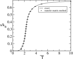
Figure 1: Entropy per site $s/k_{B}$ versus temperature ${\overline{T}}$ for the Ising model. We have used $L=N=20$ and CE intervals. The result obtained via the transfer matrix method (stars) is compared with the exact result (solid line).

The agreement between results support the adequacy of the present procedure for obtaining $s$, which will be used for estimating the temperature set.

In Table 1 we compare our temperature estimates with those obtained by Sabo et al. sabo by means of numerical integration of the specific heat $C_{v}$. The data are shown to be in good overall agreement, even though some small discrepancies can be observed at certain temperatures. They may be explained by either numerical uncertainties in the transfer matrix method, or by uncertainties in the integrations of $C_{v}$, or by derivations of $u$ in the exact method, or even by all these sources together.

CEM (exact)	CEM-S (exact)	CEM (20)	CEM-S (20)
0.1000	0.1000	0.1000	0.1000
1.4683	1.4688	1.4551	1.4635
1.6867	1.6866	1.6769	1.6820
1.8360	1.8373	1.8289	1.8332
1.9524	1.9538	1.9457	1.9496
2.0464	2.0478	2.0379	2.0433
2.1236	2.1250	2.1107	2.1201
2.1865	2.1879	2.1696	2.1836
2.2363	2.2374	2.2200	2.2386
2.2697	2.2702	2.2681	2.2883
2.3048	2.3064	2.3170	2.3365
2.3580	2.3603	2.3711	2.3896
2.4288	2.4321	2.4374	2.4518
2.5208	2.5265	2.5242	2.5341
2.6408	2.6473	2.6401	2.6464
2.8007	2.8115	2.7977	2.8019
3.0219	3.0372	3.0170	3.0220
3.3481	3.3708	3.3393	3.3483
3.8852	3.9414	3.8687	3.8847
4.9930	5.1247	4.9505	4.9906
10.000	10.000	10.000	10.000

Table 1: Temperature CEM set for the Ising model obtained from the present approach (first and third columns) and by Sabo et. al sabo (second and fourth columns).

In the first comparison among temperature schedules, we investigate the decay of time-correlation displaced functions $C_{q}$ at the critical point. This study is motivated by the fact that numerical simulations of second-order phase transitions via conventional algorithms are affected by a slow decay of $C_{q}$ (critical slowing down). On the other hand, cluster algorithms sw reduce drastically this effect. This suggests that the analysis of $C_{q}$ may be a good measure for the comparison of different criteria used in the PT. The auto-correlation function $C_{q}$ of a given quantity $q$ at the time $\tau$ is given by

$$C_{q}(\tau)=\langle(q(t)-{\bar{q}})(q(t+\tau)-{\bar{q}})\rangle/\sigma_{q}^{2},$$ (18)

where $\bar{q}$ is the mean value and $\sigma_{q}$ the variance, respectively. In Fig. 2 we plot $C_{q}$ for the thermodynamic quantities $m=\langle\sigma_{i}\rangle$ (magnetization per site) and $u=\langle{\cal H}\rangle$ (total energy per site) for all distributions described above. We have considered $R=6$ replicas ranged from ${\bar{T}}_{1}=2.269$ to ${\bar{T}}_{4}=3.660$, whose temperature set is showed in Table 2 for the CEM and ad hoc distributions. By putting the temperature set into an array, we have considered exchanges between every adjacent and non-adjacent (here between every second and third) temperatures.

CEM	ad hoc
2.269	2.269
2.345	2.400
2.464	2.580
2.658	2.830
2.996	3.170
3.660	3.660

Table 2: Temperature set of $R=6$ replicas for the Ising model obtained for the CEM and ad hoc distributions.

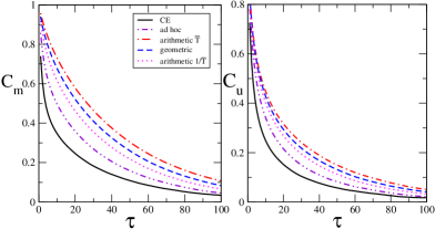
Figure 2: Time displaced auto-correlation functions $C_{m}$ and $C_{u}$ versus time $\tau$ (in MC steps) for the Ising model at the critical point for $N=L=20$ and different schemes of temperature selection.

Although all schemes give equivalent results for the steady state (for $u$ and $m$), the quantity $C_{q}$ decays faster within the CEM. As it will be shown later, a similar behavior is verified when one calculates $C_{q}$ at the critical point for the BL model. In particular, by allowing only adjacent exchanges, both $C_{m}$ and $C_{u}$ also decay faster with the CEM than other schedules.

IV.2 BEG model

We have performed numerical simulations for the BEG model in a square lattice of size $L=N=20$ using periodic boundary conditions. We focus on the analysis for ${\bar{K}}=3$, ${\bar{H}}=0$ and the low temperature ${\bar{T}}_{1}=0.5000$. In this case, a first-order phase transition between the liquids and the gas phase takes place at ${\bar{D}}^{*}=8.0000(1)$ fiore8 . Since the probability distribution at discontinuous transitions exhibit two peaks (corresponding to each phase), conventional Monte Carlo algorithms are not efficient at low temperatures, since the system requires a long time to pass from one peak to the other. In extreme cases, the peaks are separated by very high barriers and the system may get trapped in a given phase along the whole simulation and in this case it will be not ergodic. With these concepts in mind, we consider two analyses at the phase coexistence: the time evolution of the order parameter $\rho=\langle\sigma_{i}^{2}\rangle$ toward its equilibrium value $\rho_{0}=2/3$ ref20 starting from a non typical configuration and the tunneling between the phases at the coexistence after discarding sufficient MC steps. The latter study will be carried out by measuring the fluctuation of $\rho$ around $\rho_{0}$, since the trapping of the system in a given phase or in a mestastable state is expected to be signed by no relevant change of $\rho$. We have distributed temperatures between ${\bar{T}}_{1}=0.5000$ and ${\bar{T}}_{R}=2.0000$, whose entropies per site are given by $s_{1}/k_{B}=5\times 10^{-6}$ and $s_{R}/k_{B}=0.4971(1)$, respectively. By using in all cases a set of $R=6$ replicas, the CEM criterion leads to the intermediate temperatures ${\bar{T}}_{2}=1.5550$, ${\bar{T}}_{3}=1.7650$, ${\bar{T}}_{4}=1.8780$ and ${\bar{T}}_{5}=1.9400$. As for the Ising model, we have considered exchanges between every adjacent and non-adjacent (here between every second and third) temperatures. In Fig. 3, we plot the time evolution of $\rho$ starting from a lattice filled with particles. Note that by choosing the temperatures according to the CEM, the convergence of $\rho$ toward $\rho_{0}$ is faster than for other schemes. Although the results obtained for the ad hoc and CE cases are close, only in the latter scheme the system reached the steady state until $10^{5}$ MC steps.

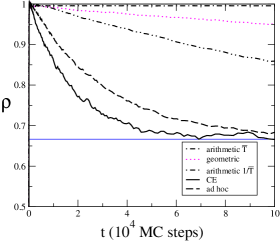
Figure 3: Time decay of the order parameter $\rho$ versus time (in MC steps) for the BEG model at the phase coexistence point (${\bar{D}}^{*},{\bar{T}_{1}}$)=($8.0000,0.5000$) for $N=L=20$ and different distribution of temperatures. The tie line for $\rho=2/3$ denotes its stationary value $\rho_{0}$.

In Fig. 4 we plot the quantity $\rho$ versus the time $t$ (in MC steps) for all procedures after discarding $1\times 10^{6}$ initial MC steps. We considered an initial configuration filled with particles and the densities are evaluated each $3\times 10^{5}$ MC steps.

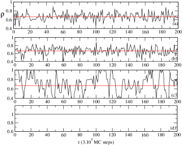
Figure 4: The density $\rho$ versus the time $t$ at the phase coexistence (${\bar{D}}^{*},{\bar{T}_{1}}$)=($8.0000,0.5000$) after discarding $10^{6}$ initial MC steps for the CEM, ad hoc, geometric and arithmetic $1/{\bar{T}}$ distributions (graphs $(a),(b),(c)$ and $(d)$, respectively). The tie lines in graphs $(a),(b),(c)$ denotes the stationary $\rho_{0}$.

With the exception of the arithmetic $1/{\bar{T}}$ criterion, where the simulation gets trapped in the liquid phase ($\rho\approx 1$) the whole time of simulation, the system is able to cross the free-energy barriers properly in the other cases. This can be viewed by the fluctuations around its equilibrium value $\rho_{0}$, whose density averages ${\bar{\rho}}$ are consistent with $\rho_{0}=2/3$ for arithmetic ${\bar{T}}$, geometric and CEM. In the next application, we shall see that the choice of the temperature interval will have more influence on the tunneling.

IV.3 Bell-Lavis model

In the last part of this paper, we study the BL model in triangular lattice of size $L=N=18$ using periodic boundary conditions. First, we repeat the analysis performed for the Ising model in the LDL-HDL second-order transition. We recall that the density of particles $\rho$ is not the order-parameter $\phi$, since $\rho\neq 0$ in both liquid phases. A previous study fiore-m showed that the appropriate $\phi$ is the difference between the fullest $\rho_{i}$ and the emptiest $\rho_{j}$ density sublattices given by $\phi=\rho_{i}-\rho_{j}$. In Fig. 5 we plot the auto-correlation functions $C_{\phi}$ and $C_{u}$ for all distributions. In particular, for the critical point located at $({\bar{\mu}_{c}},{\bar{T}_{c}}$)=($-1.000,0.430$), we distributed $R-2=4$ replicas between ${\bar{T}}_{1}=\bar{T}_{c}$ and ${\bar{T}}_{R}=0.730$, whose entropies per site are $s_{1}/k_{B}=0.5550(2)$ and $s_{R}/k_{B}=0.8763(2)$, respectively. We have also considered exchanges between every adjacent and non-adjacent (here between every second and third) temperatures. Table 3 shows the temperature set for the CEM and ad hoc cases.

CEM	ad hoc
0.4300	0.430
0.4601	0.468
0.5022	0.518
0.5589	0.576
0.6340	0.645
0.7300	0.730

Table 3: Temperature set of $R=6$ replicas for the BL model at ${\bar{\mu}_{c}}=-1.000$ obtained for the CEM and ad hoc distributions.

As in the Ising model, $C_{\phi}$ and $C_{u}$ also decay faster at the critical point when temperatures are chosen using the CEM. Repetition for other critical points leads to the same conclusion.

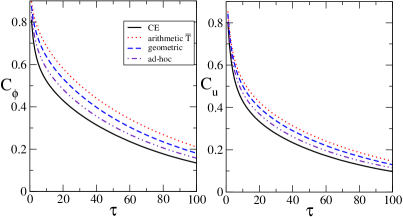
Figure 5: Time displaced auto-correlation functions $C_{\phi}$ and $C_{u}$ versus time $\tau$ (in MC steps) for the BL model at the critical point $({\bar{\mu}_{c}},{\bar{T}_{c}})=(-1.000,0.430)$ for $N=L=18$ and different temperature schedules. Results for the arithmetic $1/{\overline{T}}$ have been omitted as they are similar to the ad hoc ones.

In addition to the previous study, we also investigate the first-order phase transition gas-LDL occurring at low temperatures. Numerical simulations have been carried out at ${\bar{T}_{1}}=0.1000$. For this temperature, the phase transition takes place at ${\bar{\mu}}^{*}=-1.6500(1)$, which is identical (up to the fourth decimal level) to the transition point ${\bar{\mu}}=-1.65$ calculated at ${\bar{T}}=0$. In Fig. 6, we plot the time evolution of the density of molecules $\rho=\langle\sigma_{i}\rangle$ starting from an initial configuration filled by molecules. We consider extreme temperatures ${\bar{T}}_{1}=0.1000$ and ${\bar{T}}_{R}=0.4200$, with corresponding entropies per site given by $s_{1}/k_{B}=10^{-5}$ and $s_{R}/k_{B}=0.4604(1)$, respectively. By considering in all cases a set of $R=6$ replicas we have, for the CEM case, the intermediate temperatures ${\bar{T}}_{2}=0.2837$, ${\bar{T}}_{3}=0.3456$, ${\bar{T}}_{4}=0.3756$ and ${\bar{T}}_{5}=0.3973$.

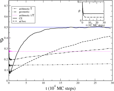
Figure 6: Time decay of the order parameter $\rho$ versus time (in MC steps) for the BL model at the phase coexistence (${\bar{\mu}}^{*},{\bar{T}_{1}}$)=($-1.6500,0.1000$) for $N=L=18$ and different distribution of temperatures. The tie line for $\rho=1/2$ denotes its stationary value $\rho_{0}$. In the inset we plot, for the ad hoc and CEM schedules, the decay of $\rho$ considering only adjacent swaps.

As for the BEG model, with the CEM the system crosses the entropic barriers more frequently than with other criteria, which can be identified by the faster convergence of $\rho$ toward its equilibrium value $\rho_{0}\approx 1/2$ fiore11 ; ref20 . On the other hand, for the other procedures, the system remains a larger number of MC steps trapped in metastable configurations and until $3\times 10^{5}$ MC steps the density has not yet converged to $\rho_{0}$. When we consider only adjacent replica exchanges, the system gets trapped in metastable states for all distributions. In the inset of Fig. 6 we plot the decay of $\rho$ only for the CEM and ad hoc schedules.

We also show in Fig. 7 the density $\rho$ versus $t$ also starting from an initial configuration filled by molecules after discarding $10^{6}$ initial MC steps.

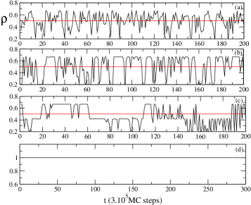
Figure 7: The density $\rho$ versus the time $t$ at the phase coexistence (${\bar{\mu}}^{*},{\bar{T}_{1}}$)=($-1.6500,0.1000$) after discarding $10^{6}$ initial MC steps for the CEM, ad hoc, geometric and arithmetic $1/{\bar{T}}$ distributions (graphs $(a),(b),(c)$ and $(d)$, respectively) and $N=L=18$. The tie lines in graphs $(a),(b),(c)$ denotes the stationary $\rho_{0}$.

In the BL model, only with the CEM and ad hoc criteria the system crosses frequently the free-energy barriers, although the tunneling is rather more frequent with the CEM than the ad hoc distribution. Only in these cases the tunneling between the different phases give an equilibrium value ${\bar{\rho}}=0.504(3)$, consistent with $\rho_{0}=1/2$. On the other hand, for arithmetic ${\bar{T}}$ (not shown) and geometric schedules the tunneling is much less frequent than the CEM ones, whereas for the arithmetic ${1/\bar{T}}$ the systems gets trapped the whole simulation in a metastable state generated by the initial configuration.

As a final remark, it is worth mentioning that the observed differences in the results yielded by the various temperature schemes are less pronounced in discontinuous transitions occurring at high temperatures. In addition, by increasing both the number of replicas and the degree of non-adjacent exchanges the results also become closer.

V Discussion and conclusion

We presented a comparative study among different protocols for the choice of the temperature set in the parallel tempering method. We focused our attention on five criteria denoted arithmetic, geometric progressions in the temperature, arithmetic progression in the inverse temperature, ad hoc distribution and the constant entropy method (CEM). In this last case, we considered an alternative direct MC method for evaluating the entropy which avoids numerical integrations of the specific heat or other thermodynamic quantities. We have considered rather few number of replicas ($R=6$ for continuous and discontinuous phase transitions) and adjacent and non-adjacent replica exchanges. Different systems undergoing first and second-order phase transitions have been undertaken. In all cases, the temperature selection via the difference of entropy method revealed more advantageous. More specifically, at the criticality (where configurations generated by standard algorithms become strongly correlated) the time displaced correlation functions decay faster when temperatures are chosen with the CEM. This behavior can be understood that near criticality (where a small change of temperature provoke a large change of entropy) the CEM gives more concentrated intermediate temperatures than all distributions. Thus, replicas at the lowest temperature (${\bar{T}}={\bar{T}_{1}}$) display a larger probability of exchanging configurations than the other cases. Since the time correlation decays faster for ${\bar{T}}>{\bar{T}_{c}}$ than ${\bar{T}}={\bar{T}_{c}}$, the more frequent exchanges provide the system at ${\bar{T}_{1}}$ decays faster. For discontinuous transitions at low temperatures, where high entropic barriers do not allow the system to cross the phase frontiers properly (also when simulated by conventional algorithms) and hence the choice of the adjacent temperatures may play a crucial role, the CEM has also offered a rather efficient recipe for determining the temperature set. Within the CEM the lower temperatures are more sparse than with other schemes and, though unlikely, a successful replica exchange allows the system to evolve to configurations which are able to cross the high free energy barriers faster than other distributions. We have also distributed temperatures following an ad hoc scheme, in such a way that the exchange probability between adjacent replicas was about 30$\%$. Although this method has shown to be more efficient than arithmetic and geometric schedules at the phase transition, it is inferior than the CEM. In summary, our comparative study ellects the CEM as an useful tool for obtaining the temperature schedule to be used in numerical simulations of phase transitions through the parallel tempering method.

VI Acknowledgments

I acknowledge Renato M. Ângelo, Mauricio Girardi, Sergio D’Almeida Sanchez and Marcos G. E. da Luz for critical readings of this manuscript and the financial support from CNPQ.

References

- (1) K. Hukushima and K. Nemoto, J. Phys. Soc. Jpn. 65, 1604 (1996); C. J. Geyer, Markov-Chain Monte Carlo maximum Likehood, Comp. Sci. and Stat., p. 156 (1991).
- (2) E. Marinari and G. Parisi, Europhys. Lett. 19(6), 451 (1992).
- (3) K. Binder and W. Kob, Glassy Materials and Disordered Solids: An Introduction to their Statistical Mechanics (World Scientific, Singapoure, 2005).
- (4) J. Skolnick and A. Kolinski, Comput. Sci. Eng. 3(9/10), 40 (2001).
- (5) D. A. Kofke, J. Chem. Phys 117, 6911 (2002).
- (6) C. Predescu, M. Predescu and C. Ciobanu, J. Chem. Phys. 120, 4119 (2004); J. Phys. Chem, B 109, 4189 (2005).
- (7) A. Kone and D. A. Kofke, J. Chem. Phys 122, 206101 (2005).
- (8) H. G. Katzgraber, S. Trebst, D. A. Huse and M. Troyer, J. Stat. Mech. 3, P031018 (2006).
- (9) D. Sabo, M. Meuwly, D. L. Freeman and J. D. Doll, J. Chem. Phys 128, 174109 (2008).
- (10) D. Sabo, private communication (2011).
- (11) F. Calvo, J. Chem. Phys. 123, 124106 (2005).
- (12) R. A. Sauerwein and M. J. de Oliveira, Phys. Rev. B, 52, 3060 (1995).
- (13) E. Ising, Z. Phys. 31, 253 (1925).
- (14) M. Blume, V. J. Emery, and R. B. Griffiths, Phys. Rev. A 4, 1071 (1971), W. Hoston and A. N. Berker, Phys. Rev. Lett. 67, 1027 (1991).
- (15) G. M. Bell and D. A. Lavis, J. Phys. A 3, 568 (1970).
- (16) N. Metropolis, A. W. Rosenbluth, M. N. Rosenbluth and A. H. Teller, J. Chem. Phys. 21, 1087 (1953).
- (17) J. P. Neirotti, F. Calvo, D. L. Freeman and J. D. Doll, J. Chem. Phys. 112, 10340 (2000).
- (18) F. Calvo, J. P. Neirotti, D. L. Freeman and J. D. Doll, J. Chem. Phys. 112, 10350 (2000).
- (19) C. E. Fiore, Phys. Rev. E 78, 041109 (2008).
- (20) C. E. Fiore and M. G. E. da Luz, Phys. Rev. E 82, 031104 (2010).
- (21) C. E. Fiore and M. G. E. da Luz, J. Chem. Phys 133, 104904 (2010).
- (22) B. Kaufman, Phys. Rev. 76, 1232 (1949); A. E. Ferdinand and M. E. Fisher, Phys. Rev. 185, 832 (1969).
- (23) K. Binder and D. W. Heermann, Monte Carlo Simulation in Statistical Physics (Springer-Verlag, New York Berlin Heidelberg, 1992).
- (24) C. E. Fiore, M. M. Szortyka, M. C. Barbosa and V. B. Henriques, J. Chem. Phys 131, 164506 (2009).
- (25) R. H. Swendsen and J. S. Wang, Phys. Rev. Lett. 58, 86 (1987), U. Wolff, Phys. Rev. Lett 62, 361 (1989).
- (26) C. E. Fiore, V. B. Henriques and M. J. de Oliveira, J. Chem. Phys. 125, 164509 (2006).
- (27) H. C. M. Fernandes, J. J. Arenzon and Y. Levin, J. Chem. Phys. 126, 114508 (2007).
- (28) C. E. Fiore and C. E. I. Carneiro, Phys. Rev. E 76, 021118 (2007).
- (29) For the BEG model, the equilibrium value for at the phase coexistence can be understood recalling that two liquid phases () coexist with one gas phase (). Since their weights are equal (1/3), we have for any system size. A similar reasoning shows for the BL model at the phase coexistence.