Temporal Deconvolution study of Long and Short Gamma-Ray Burst Light curves

Abstract

The light curves of Gamma-Ray Bursts (GRBs) are believed to result from internal shocks reflecting the activity of the GRB central engine. Their temporal deconvolution can reveal potential differences in the properties of the central engines in the two populations of GRBs which are believed to originate from the deaths of massive stars (long) and from mergers of compact objects (short). We present here the results of the temporal analysis of 42 GRBs detected with the Gamma-ray Burst Monitor onboard the Fermi Gamma-ray Space Telescope. We deconvolved the profiles into pulses, which we fit with lognormal functions. The distributions of the pulse shape parameters and intervals between neighboring pulses are distinct for both burst types and also fit with lognormal functions. We have studied the evolution of these parameters in different energy bands and found that they differ between long and short bursts. We discuss the implications of the differences in the temporal properties of long and short bursts within the framework of the internal shock model for GRB prompt emission.

1 Introduction

The temporal structure of GRB light curves exhibits very diverse morphologies, from single pulses to extremely complex multi-pulse structures. As a result, morphological GRB classification attempts have not been successful and the only established division of bursts into classes with different temporal characteristics is based on their durations (Kouveliotou, et al.,, 1993). The latter have been found to distribute bimodally, with over 75% of the events belonging in the long class ($>2$ s) when durations are measured in the 50-300 keV range. Since 1993 the GRB durations are mostly measured by their $T_{90}$ ($T_{50}$) intervals, the times during which 90% (50%) of the total event counts (or fluence) are collected (Kouveliotou, et al.,, 1993). McBreen et al., (1994) and later Horváth, (2002), showed that durations ($T_{90}$) of both long and short GRBs follow lognormal distributions separately. Several authors have studied the deconvolution of GRB light curves into their constituents, and have shown that in general, these are discrete, often overlapping pulses with durations ranging from a few milliseconds to several seconds and almost always asymmetric shapes, with faster rises than decays (Norris et al.,, 1996; Hakkila and Preece,, 2011). These highly varied GRB temporal profiles are suggestive of a stochastic process origin.

Two distinct mechanisms have been proposed to explain the origin of pulses in GRBs. In the external shock model, radiation pulses are emitted when a relativistic shell ejected by the GRB central engine is decelerated by the circum-burst material (Mészáros and Rees,, 1993). A homogeneous medium leads to a single pulse but an irregular, clumpy environment can produce a complex profile if a large number of small clouds are present (Dermer and Mitman,, 1999). According to the internal shock model (Rees and Mészáros,, 1994), the central engine generates relativistic shells with highly non-uniform distribution of Lorentz factors and the pulses are formed by the collision between a rapidly moving shell with a slower shell. Thus in principle the variability of the GRB light curves may directly correspond to the activity of their central engines (Daigne and Mochkovitch,, 2003; Nakar and Piran,, 2002). Hence the studies of pulse properties are important to determine whether GRB sources require engines that are long lasting or impulsive (Dermer,, 2004).

Investigations linking GRB properties with their pulse characteristics have already been carried out by several authors (Norris et al.,, 1996; Li and Fenimore,, 1996; Quilligan et al.,, 1999; Lee, Bloom and Petrosian,, 2000; McBreen et al.,, 2001; Hakkila and Cumbee,, 2008). Norris et al., (1996) were the first to deconvolve the profiles of long and bright GRBs detected with the Burst And Transient Source Experiment (BATSE) onboard the Compton Gamma Ray Observatory (CGRO) into pulses and study the pulse shape parameters as a function of energy. Gupta et al., (2000) were the first to fit lognormal functions to pulses in short GRBs detected with BATSE. McBreen et al., (2001) applied a pulse identification algorithm on a set of BATSE short bright bursts and derived their pulse shape parameters; they concluded that the pulse rise and decay times follow lognormal distributions. However, the BATSE GRB light curves used in these studies had a time resolution of 64 ms for long bursts, which could have masked narrower pulses in those bursts. However the short burst studies have been carried out using higher resolution data.

A long standing question has been, therefore, whether the representative time scales associated with pulses of long GRBs form a separate class from those in short bursts perhaps reflecting the two different prevalent models for their origin, i.e., long bursts originate from the collapse of massive stars (Woosley and Heger,, 2006; Woosley and Bloom,, 2006), while short GRBs result from the merger of two compact objects (Eichler et al.,, 1989; Narayan $et~{}al.$,, 1992). If we could deconvolve the GRB light curves in terms of simpler pulse shapes, we could potentially identify the differences in the central engines of long and short GRBs. In this paper, we show that there is a fairly high degree of determinism underlying the complex nature of the GRB temporal profiles. In § 2 we describe the instrument and the selection criteria for our sample, and in § 3 we expand on our analysis technique. In § 4 we decompose the high-time resolution GRB data of the Gamma-ray Burst Monitor (GBM) onboard the Fermi Gamma-ray Space Telescope (hereafter Fermi) into individual pulses and examine the distributions of the pulse shape parameters for long and short duration GRBs. Further we apply the same analysis technique to GRB light curves in various energy bands and study the pulse shape evolution with energy. We discuss our results in § 5.

2 Instrumentation and Data Selection

GBM is an uncollimated all-sky (field of view $\geq$ 8 sr) monitoring instrument. It consists of an array of 12 NaI(Tl) scintillation detectors mounted in clusters of three around the spacecraft. Each NaI(Tl) detector is 12.7 cm in diameter by 1.27 cm thick, and covers an energy range from 8 keV to 1 MeV. In addition, GBM includes two Bismuth Germanate (BGO) detectors, each 12.7 cm in diameter by 12.7 cm thick, placed on either side of Fermi. The BGOs cover energies above 150 keV up to a maximum of 40 MeV (Meegan et al.,, 2009).

The GBM on-board software incorporates burst triggering on time scales as short as 16 ms. All triggers generate time-tagged event data (TTE) consisting of the photon arrival time and energy as deposited from each of the 14 detectors with a temporal resolution of 2 $\mu$s (Meegan et al.,, 2009). The very high temporal resolution and large energy band-width are major assets for the study of GRBs in general and the study of short events, in particular. A pre-burst ring buffer saves about half a million events before the trigger, which corresponds to a time interval of $\sim$30 seconds. The TTE data are produced for $\sim$300 seconds after the trigger. All short bursts and a bulk of the long bursts have full temporal coverage by TTE data. The energy range for both NaI and BGO detectors is digitized into 128 channels, pseudo-logarithmically spaced to provide channel widths less than each detector energy resolution up to 12 MeV though TTE data are available at coarser resolution up to 40 MeV. During the 3 years since its launch (2008 June 11) GBM has collected over 700 GRBs. During the first year GBM detected 225 GRBs of which 59 were BGO bright bursts (Bissaldi,et al.,, 2011). This is to ensure the burst is sufficiently hard to allow pulse decomposition analysis in different energy channels. Out of the latter dataset we chose long bursts with the product of fluence and peak flux (1.024s) values greater than $1.0\times 10^{-4}$ and $5.0\times 10^{-6}\,{\rm erg~{}ph/cm^{4}/s}$ for long and short bursts respectively. Burst fluences and peak fluxes estimated in the energy range 10-1000  keV are taken from the GBM Gamma-ray burst catalog (Paciesas, et al.,, 2011). As a result, the final sample includes 32 long bursts with fluences ranging from $5.5\times 10^{-6}$ to $2.7\times 10^{-4}\,{\rm erg/cm^{2}}$ and 10 short bursts with fluences ranging from $8.5\times 10^{-7}$ to $8\times 10^{-6}\,{\rm erg/cm^{2}}$. This unusual selection criteria is simply to eliminate weak and long bursts with fluences above the threshold that are difficult for the pulse decomposition analysis. We have also used the BGO data in the current analysis. The burst durations and the number of fitted pulses are listed in Table 1. Possible selection effects arising from our choice of burst sample is assumed to be small in the present analysis.

For each burst we summed the TTE data of the four NaI detectors that registered the highest gamma-ray signal (with an angle to the burst direction of $\leq$ 60$\arcdeg$) to derive their light curves with a resolution of 1 ms. In the case of BGO detectors, the light curves from both the detectors were summed. Each light curve included the entire burst and background regions up to about 10-20 s before and after the burst. We varied the temporal resolution used for the analysis depending on the burst intensity (see next section for details). The analysis described below was performed on the entire energy range of NaI ($8-1000$ keV) and BGO ($0.15-45.0$ MeV) detectors as well as in six NaI energy ranges per burst ($8-520$ keV; see also Table 2). It may be noted that there are uncertainties in the energy edges listed in Table 2 that arise primarily from the finite energy resolution of the GBM detectors (Meegan et al.,, 2009).

3 Analysis Technique

In general, a parameter which can be written as a product of $\geq$ 3 random variables tends to follow a lognormal function (Aitchison and Brown,, 1969). Since the pulse shape parameters of GRB light curves can be described as such a product, we were motivated to use a similar procedure to test this hypothesis (Ioka and Nakamura,, 2002). Ioka and Nakamura, (2002) argue that the distribution of a product of variables tends to the lognormal distribution as the number of multiplied variables increases, the distribution of pulse width may be closer to the lognormal distribution than that of the pulse intervals between successive pulses. It has already been shown that the long and short GRB durations, the time interval between successive pulses (McBreen et al.,, 1994), fluence and pulse intervals between successive pulses within each burst (Li and Fenimore,, 1996), pulse durations (Nakar and Piran,, 2002) and spectral break energies (Preece, et al.,, 2000) do follow lognormal distributions.

We also choose a lognormal function to fit pulses in a GRB light curve. A lognormal function in this case has 4 free parameters, namely the amplitude (A), mean ($\mu$), standard deviation ($\sigma$) and time. The advantage of choosing this functional form is that it converges in all cases even when the shape of the light curve is very complex, where the pulses are often overlapping. The pulse shape parameters are derived from the fit parameters using the following formulations.

A lognormal function is represented as:

$$f(x)=\left\{\begin{array}[]{ll}\frac{A}{\sqrt{2\pi}x\sigma}\exp\left[-\frac{(\log~{}x-\mu)^{2}}{2\sigma^{2}}\right]&{\rm if}~{}x>0\\ &\\ 0&{\rm if}~{}x\leq 0\\ \end{array}\right.$$

where, $\mu$ and $\sigma$ are the sample mean and standard deviation of $\log{x}$, and A is the amplitude. The rise time, $\tau_{r}$, decay time, $\tau_{d}$, and the full width at half maximum of each pulse, FWHM, can be derived from the fit parameters of the lognormal function given above. The rise and decay times are measured from the time differences at 10% and 90% of the peak amplitude of a pulse.

$$\tau_{r}=\exp{(\mu-\sigma^{2})}\left[\exp\left(-\sigma\sqrt{2\log\left(\frac{10}{9}\right)}\right)-\exp\left(-\sigma\sqrt{2\log{(10)}}\right)\right]$$

$$\tau_{d}=\exp{(\mu~{}-~{}\sigma^{2})}\left[\exp\left(\sigma\sqrt{2\log{(10)}}\right)-\exp\left(\sigma\sqrt{2\log\left(\frac{10}{9}\right)}\right)\right]$$

$$FWHM=\exp{(\mu~{}-~{}\sigma^{2})}\left[\exp\left(\sigma\sqrt{2~{}\log{(2)}}\right)-\exp\left(-\sigma\sqrt{2~{}\log{(2)}}\right)\right]$$

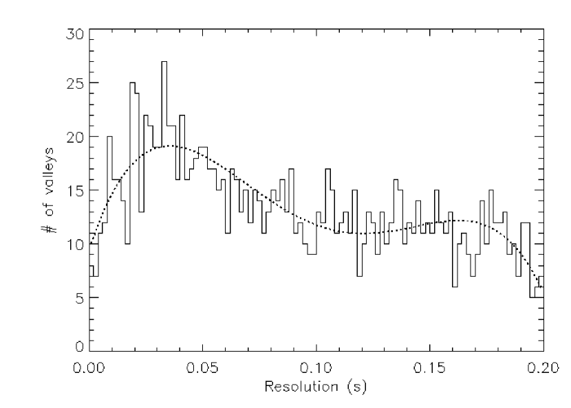
Figure 1: A sample histogram of the number of valleys identified by an algorithm based on the method suggested by Li and Fenimore, (1996), as a function of bin-width of the light curve for GRB 080723D. The number of valleys increases initially and reaches a broad maximum at the optimum bin-width (25-50 ms)and then gradually falls at very coarse resolution. The curve is a ploynomial fit to guide the eye only. The number of valleys and the bin-width at the maximum agrees with that chosen for this GRB which is 18 valleys at a time resolution of 50 ms.

For each GRB we initially selected the number of possible pulses contained in the light curve by visually identifying the significant valleys on either side of a pulse. This process was repeated for each burst varying the temporal resolution of the summed light curve until the number of valleys reached a maximum. If the resolution was too fine, the pulses were burried in statistical fluctuations and hence the number of identified valleys was too small. At very coarse resolutions the closely spaced pulses merged with each other also resulting in a reduced number of valleys. The number of valleys is maximum at the optimum temporal resolution for a given burst. Figure 1 shows such a histogram where the number of valleys identified automatically by a routine based on the technique of Li and Fenimore, (1996), as a function of bin-width of GRB light curve. The number of valleys increases initially with increasing binwidth and then reaches a broad maximum at a resolution in the range 25-50 ms and then falls gradually with further increase in the bin-width. The number valleys estimated manually for this burst was 18 at a chosen optimum bin-width of 50 ms which agrees well with those estimated objectively. The mean time resolution for all the GRBs in our sample is $\sim$ 40 msec.

The array of valleys was then used as input to the pulse fitting routine. It generates initial guesses of the amplitudes, means and the standard deviations based on the number of counts in the light curve between a pair of valleys while the pair of valleys are used to estimate the initial guess of time parameter. The routine then simultaneously fitts lognormal functions to pulses at optimum times and a quadratic to the background. It compared the model light curve with the data and minimized its $\chi^{2}$ value by varying the pulse shape parameters and the position of the pulses. The goodness of fit, $n$, was finally calculated by computing the likelihood parameter as -2$\ln\pounds$ (which approaches Pearson’s $\chi^{2}$ for large model values) divided by the number of degrees of freedom (dof). The number of dof is the difference between the number of data points in the light curve minus the total number of fitted parameters. This procedure was then repeated for the light curves in the first four to six energy bands (depending on the burst intensity in the higher energy bands) shown in Table 2, defined so that a typical GRB light curve had similar signal to noise ratio in each channel. After pulse fitting we used the pulse mean positions to compute the intervals between successive pulses, while the variation of the pulse shape parameters in different energy bands were used to study the spectral evolution of the pulse shapes. The pulse mean positions refer to the mean times(with respect to the trigger time) of the lognormal pulses.

To test the integrity of the fit we computed a weight for each of the fitted pulses in a light curve by estimating the percentage change in the goodness of fit parameter with that pulse excluded. Pulses with weights less than 2% were excluded from the fit as they most likely were due to statistical fluctuations. The overall goodness of fit did not change more than 10% compared to its value before any pulse rejection. No case was found where an additional pulse was needed to improve the residuals. Thus the pulse fitting procedure was optimized to ensure removal of spurious pulses.

To check the robustness of our fits, we also performed a series of simulations as follows. We chose a set of pulses fitted to a light curve and generated a synthetic light curve using these pulses superposed over the burst fitted background. We then reduced the light curve intensity in steps of 10%, starting at 100%, and added statistical noise to each bin. Each light curve was fitted by the normal procedure and recovered entirely until the intensity was decreased to 50%. The degree of percentage recovery declined thereafter, and reached 75% of the original, when the intensity was reduced to 10% of the total. We concluded that the fit is robust for a large range of burst intensities.

Further we reduced the duration of the simulated burst by a factor and fitted the light curve with the lognormal functions as before. Each time the separation between the pulses too reduced by the same factor. Hence there was no lower limit on the inter-pulse separation caused by the closeness of the successive peaks in the light curve. This was tested by reducing the burst duration by a factor of 1000.

Finally, to address the issue of the interdependency of the rise and decay times of a lognormal function we tried two new functions, where these times can vary independently. They are:

$f_{1}(x)=\frac{A}{(\tau_{d}-\tau_{r})}\left[\exp(-\frac{x}{\tau_{r}})-\exp(-\frac{x}{\tau_{d}})\right]$, (Leo,, 1994)

$f_{2}(x)=A\lambda\,\exp(-\frac{\tau_{1}}{x}-\frac{x}{\tau_{2}})\ {\rm for\ }x\,>\,0$, (Norris et al.,, 2005)

where $\lambda=\exp(2\mu)$ and $\mu=\left(\frac{\tau_{1}}{\tau_{2}}\right)^{\text@frac{1}{2}}$.

We find that for long bursts with a small number of pulses, both the above functions fit the light curve as well as the lognormal function. However, in case of bursts with complex light curves consisting of several overlapping narrow pulses, these functions fit poorly resulting in large $\chi^{2}$ compared to a fit with a lognormal function. Since the present analysis aims at a comparison of the pulse properties of long and short bursts, we opted to use the lognormal function, which describes the light curve best in all cases.

4 Results

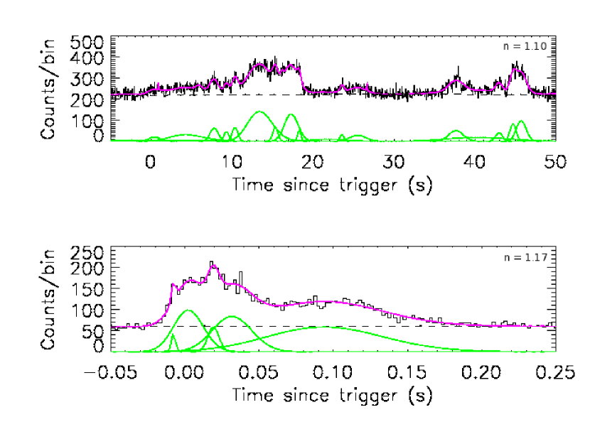
Figure 2: A sample pulse fit to one long burst GRB 080723D (upper plot) and one short burst GRB 090227B (lower plot). The histogram in black is the GRB light curve and the fitted background is shown as black dashed line. The pulses shown in green are the lognormal pulses fitted to those in the light curves. The sum of the background model and the fitted pulses is shown as purple continuous line. The goodness of fit parameter, $n$, is indicated at the top right corner of each plot.

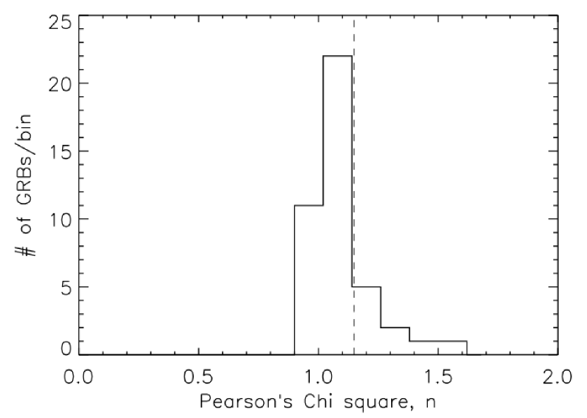
Figure 3: A distribution of the goodness of fit parameter n, viz. Pearson’s chisquare estimated from the liklihood ratio for each fit. The vertical dashed line shows the mean value of the entire sample.

We performed the analysis described above on all 42 GRBs in our sample. The pulse shape parameters from the analyses of the entire sample of light curves used here are summarized in 2 tables which are available in the online version of this paper. Figure 2 shows an example of fitted pulses to light curves of one long (GRB 080723D, upper plot) and one short (GRB 090227B, lower plot) GRB. The quality of each fit, $n$, is indicated at the top right hand corner of each panel. The mean value of this parameter for all the 42 fits is 1.15 with a standard deviation of 0.13. Figure 3 shows the distribution of $n$. We note that it peaks around 1, as expected since $n$ is expected to follow the $\chi^{2}$ distribution.

4.1 Pulse shape parameters

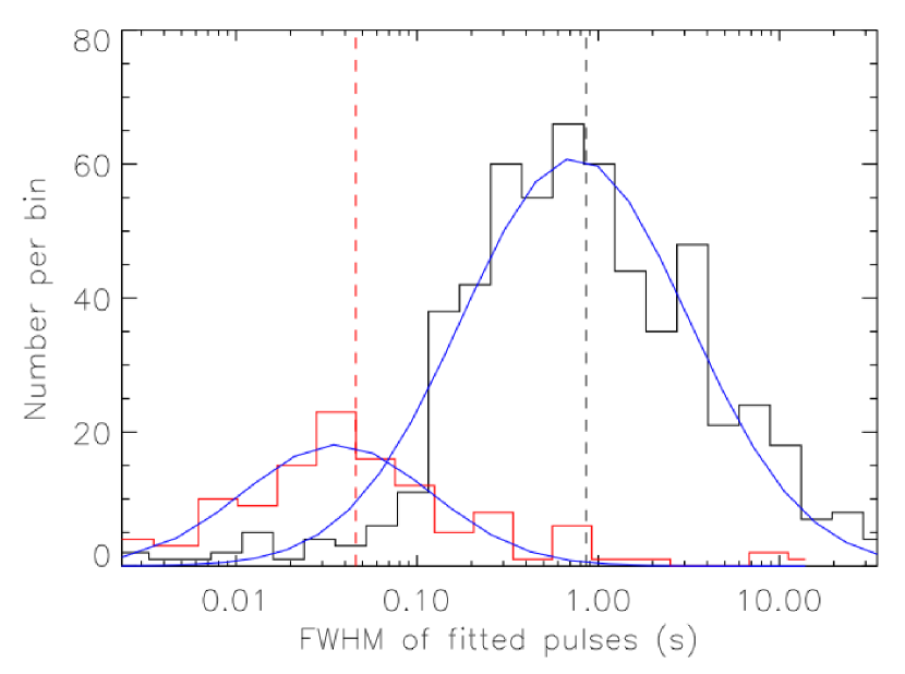
Figure 4: Distributions of the pulse widths (FWHM) for long (histogram shown in black) and short bursts (histogram shown in red). A lognormal function is fitted to each of the distributions. The mean values of FWHM (from the fit) for long and short bursts are 0.89 s and 0.055 s and the standard deviations are 5.2 s and 4.6 s respectively. The vertical dashed lines are the median values of FWHM for each class of GRBs.

For each burst, we derived $\tau_{r}$, $\tau_{d}$ and $FWHM$ for every fitted pulse from the formulae listed in the previous section. Figure 4 shows the distributions of pulse FWHM for long and short bursts also independently fitted with lognormal functions with mean values of pulse widths of 0.95  s and 0.06  s, respectively. The distributions are overlapping but distinct for the two types of bursts. We note that short burst light curves consist of distinctly narrower pulses compared to long GRBs.

The pulse widths and intervals between successive pulses are primary attributes which could ultimately reveal important clues about GRB physics. Figure 5 shows the distributions of the time intervals ($\Delta t$) between adjacent pulse positions for long and short GRBs. Again we fit the distributions independently with lognormal functions. The means of the fitted lognormal functions are 1.6 s and 0.08 s for long and short bursts, respectively. The pulses in short bursts are about 20 times more closely spaced than those in the long bursts. The range of intervals between successive pulses spans nearly 3 decades both for long and short GRBs consistent with the earlier results for BATSE bursts (Norris et al.,, 1996). An exponential function does not fit the cumulative distributions of the intervals between successive pulses well, indicating that most likely the GRB pulses do not follow a Poisson distribution in time.

It may be noted that the average redshift of short bursts is smaller than that of long bursts (see section 5). Hence the average pulse widths and and intervals between successive pulses of long bursts could be larger by a factor of 1.74 because of this effect. However the redshift effect is too small to account for the separation between them as seen in figures 4 and 5.

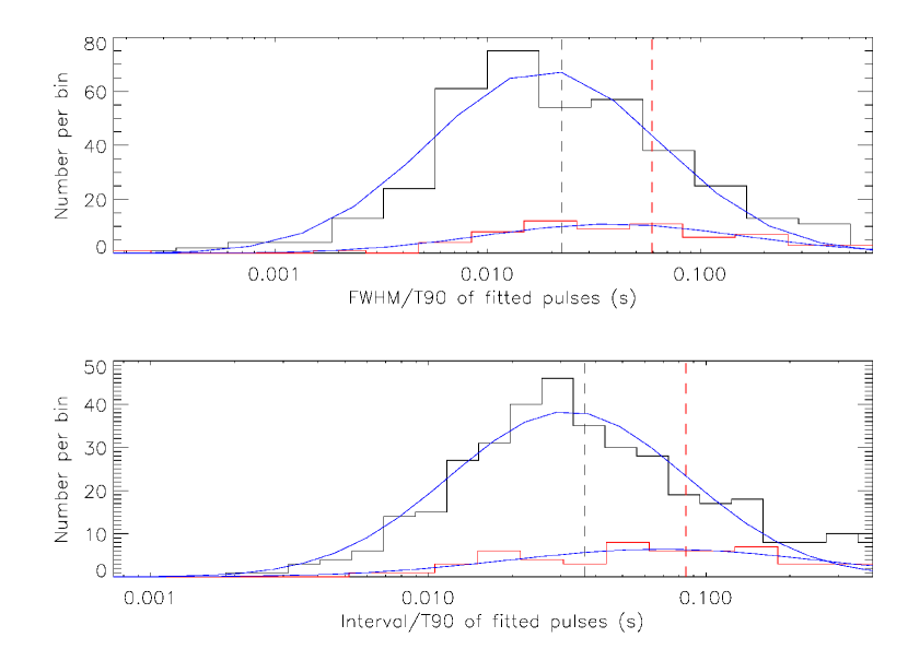
Figure 6: Distributions of the ratio of pulse widths (FWHM) of a burst to its total duration, $T_{90}$, for long bursts (histogram in black) and short bursts (histogram in red, upper panel). Each of the histograms is fitted with a lognormal function (shown as continuous curves in blue). The vertical dashed lines show the median values for long and short bursts respectively. The lower panel shows similar distributions of the ratio of the GRB time interval between successive pulses and the burst duration ($T_{90}$). Considering large errors in the short burst durations the two distributions may be considered to be consistent with each other in both the cases. The lag between the two distributions are $1.0\pm 0.7$ (upper plot) and $2.0\pm 0.7$ bins (lower plot)

To compare the pulse width contribution to the total duration in short and long bursts, we derive the ratio of the pulse width (FWHM) to the $T_{90}$ of each burst. Figure 6 (top panel) shows the histograms of these ratios for long and short bursts. Also shown are the median values of these distributions. The same figure (lower panel) shows similar distributions for the ratio of the pulse time intervals between successive pulses and the burst durations again for both burst types. The distributions for long and short bursts are overlapping and consistent with each other, considering large uncertainties in the short burst durations (Table 1). In order to quantify the degree of overlap we estimated the time lag between the two distributions as follows. We estimate the cross-correlation coefficient (CC) as a function of lag between the two histograms. It is found that maximum of the CC values are 0.94 and 0.91 respectively for the distributions implying that the corresponding distributions for long and short bursts are correlated. The lag is defined as its value where the CCF peaks. In addition, we estimated lag 100 times for each pair of histograms while adding Poisson noise to the data each time. The standard deviation of the lags from the simulated histograms is the error on the estimated lag. The lags so estimated are $1.0\pm 0.7$ bins and $2.0\pm 0.7$ bins for the two distributions respectively. The values of lags are close to zero supporting the general observation that the short GRBs are similar to long GRBs compressed in time (Guiriec, et al., 2010).

We now compare the GBM results with those of the BATSE bursts. Nakar and Piran, (2002) use a modified peak finding algorithm first reported by Li and Fenimore, (1996), to a sample of 68 long BATSE bursts and report that the pulse durations follow a lognormal distribution. The pulse interval distribution which peaks around an interval of 1.0 s also exhibits an excess of longer intervals between successive pulses with respect to a lognormal function. This is consistent with the analysis of 319 long bright BATSE GRBs by Quilligan et al., (2002). They show that for long GRBs the distribution of intervals between successive pulses peak at 1 s and intervals longer than 15 s, which form 5% of the total, do not fit the lognormal distribution. They also show that these intervals between successive pulses are consistent with a power law. The origin of this excess has been attibuted to the existence of quiescent times between successive peaks. In the present data, the distribution of pulse intervals for long bursts peaks around 1 s and the fraction of intervals between successive pulses above 15 s is $(3.8\pm 0.8)$% which is consistent with the above result. The interval distributions for both long and short bursts are best fit by lognormal functions (Figure 5). The lognormal fit for long bursts shows a hint of an excess of long intervals between successive pulses even though statistically not compelling because of smaller number of bursts in our sample.

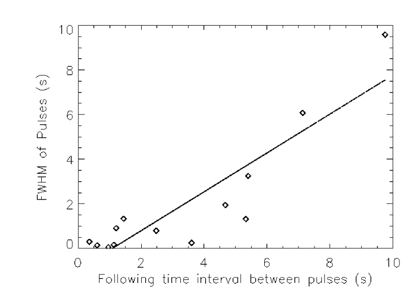
Figure 7: A plot of the pulse FWHM as a function of following time interval between successive separable pulses for a long burst GRB090626 which show a linear correlation coefficient of 0.896. The null hypothesis probability is $2.4\times 10^{-4}$ after taking into account of the number of GRBs searched (7 in this case). The black dashed line shows a linear fit to the data points.

Nakar and Piran, (2002) find a positive correlation ($>$ 70%)between pulse width and the preceding interval and a weaker correlation between pulse width and the following time interval. They considered only bursts with more than 12 well separated pulses and the total number of long bursts in their sample meeting this criteria was 12. There are 7 long bursts meeting these criteria in our sample. A search for such a correlation in our GRB sample has been carried out. In addition, we also searched for possible correlations between the pulse amplitude and the preceding or following time interval. We found one case of significant correlation (for GRB090626A) between the pulse width (FWHM) and the following time interval between successive pulses. The Pearson’s linear correlation coefficient is 0.896 with a statistical null hypothesis probability of $2.42\times 10^{-4}$. The corresponding plot is shown in Figure 7. We found good correlations in a few other cases. However these correlations were found to be contributed by one or two deviant points and hence likely to be spurious. No significant correlations were found between the pulse amplitude and the time intervals in any burst in our limited sample. It seems that there are certain types of long bright GRBs which show such correlation between the pulse width and following time interval between successive separable pulses. The implications of these correlations is not clear at present.

4.2 Spectral Evolution of Pulse Shape Parameters

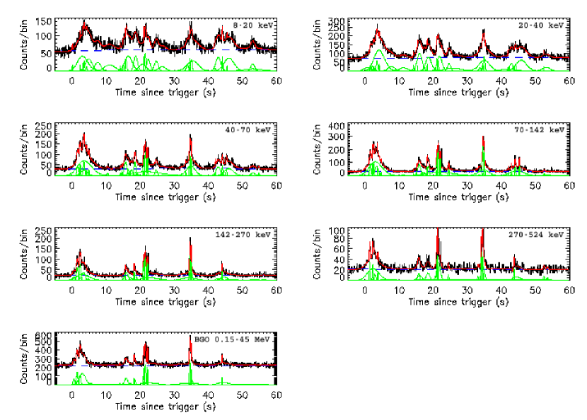
Figure 8: Sample pulse fits to the lowest 6 energy channels of NaI and the full energy range light curve from BGO detector of a long GRB 090626A. The histogram in black is the GRB light curve with a time resolution of 50 ms. The pulses shown in green are fitted lognormals to those in the GRB light curve. The horizontal dashed blue line is the fitted background while red curve is the fitted light curve resutling from summing the green and black curves. The temporal features in the light curve and hence the fitted pulses are narrower at higher energies.

Figure 8 shows a set of light curves of GRB 090626A in 7 different energy bands. Here we were restricted by the statistics in the higher energy channels, which did not allow reliable pulse fitting beyond 524 keV for many bursts. The histograms of the pulse shape parameters were generated as above in each energy range for short and long bursts. We assigned a mean energy for each range estimated as the geometric mean of the energy boundaries of each band. The energy range of each light curve is indicated on each plot. The bottom panel is from a fit to the BGO light curve of the same burst in the entire BGO energy range. As in figure 2 the individual pulses shown at the bottom of each panel when superposed on the quadratic background (shown as dashed line) describe the burst light cuve shown as continuous line in red. Table 3 lists the number of pulses fitted for a smaple of long GRBs in different energy bands. There does not seem to be a drastic change in the number of fitted pulses in the NaI energy range. The pulse fitting analysis of the BGO light curves in various energy bands were limited to very few bursts and hence the results from the analysis of full energy light curves only are used here.

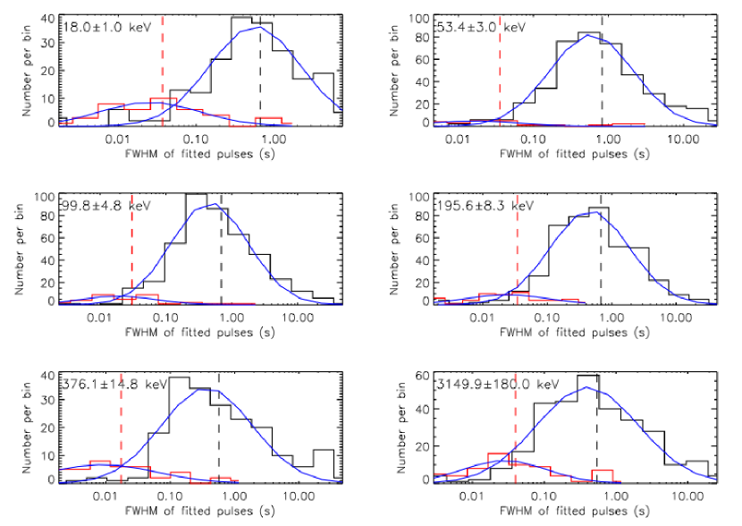
Figure 9: Evolution of the distributions of pulse widths for long (histogram shown in black) and short (histogram shown in red) GRBs as a function of energy. The first 5 distributions are from the NaI light curves in the first five energy bands as shown in Table 2. Also shown in the lowest right panel is a similar distribution for the total energy light curve from the BGO detector. The histograms for long and short bursts are fitted to lognormal functions and shown as continuous curves (in blue) in each energy band. The geometric mean energies corresponding to each plot are indicated in each panel. The errors on the mean energies are due to the finite energy resolution of GBM detectors.

Figure 9 shows the distributions of pulse width (FWHM) of long and short GRBs in different energy ranges. The distributions in each energy band are well fit (shown as continuous curves) by lognormal functions. The width of the fitted lognormals, as well as the values where the distributions peak, do not seem to change significantly with energy. The largest differences appear when we compare the two extreme energy bands, namely between 18  keV and $\sim$ 3.15 MeV, with the latter widths being 0.04 s and 0.5 s narrower, for short and long GRBs, respectively.

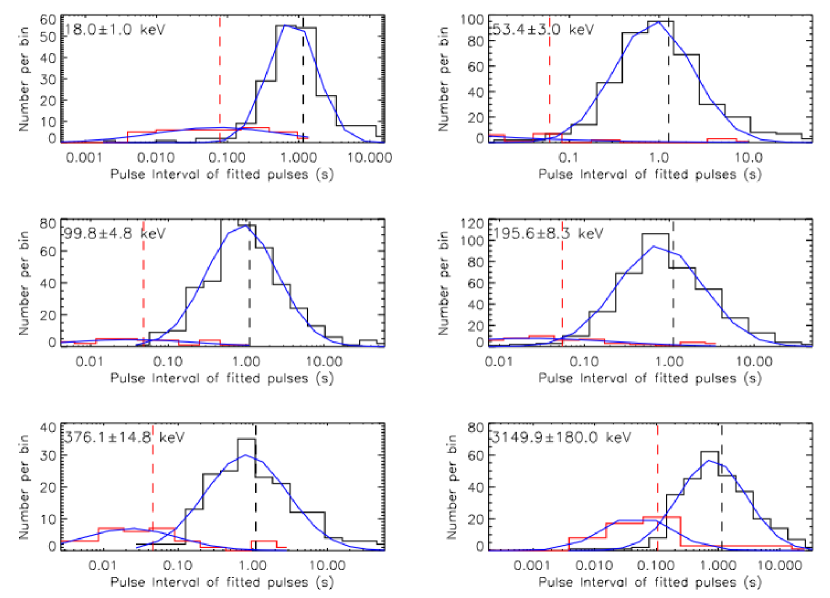
Figure 10: Evolution of the distributions of pulse time intervals between successive pulses for long (histogram shown in black) and short GRBs (histogram shown in red) as a function of energy. The first 5 distributions are from the light curves in the first five energy bands as shown in Table 2. Also shown in the lowest right panel is a similar distribution for the total energy light curve from the BGO detector. The histograms for long and short bursts are fitted to lognormal functions and shown as continuous curves (in blue) in each energy band. The geometric mean energies corresponding to each plot are indicated in each panel. The errors on the mean energies are due to the finite energy resolution of GBM detectors.

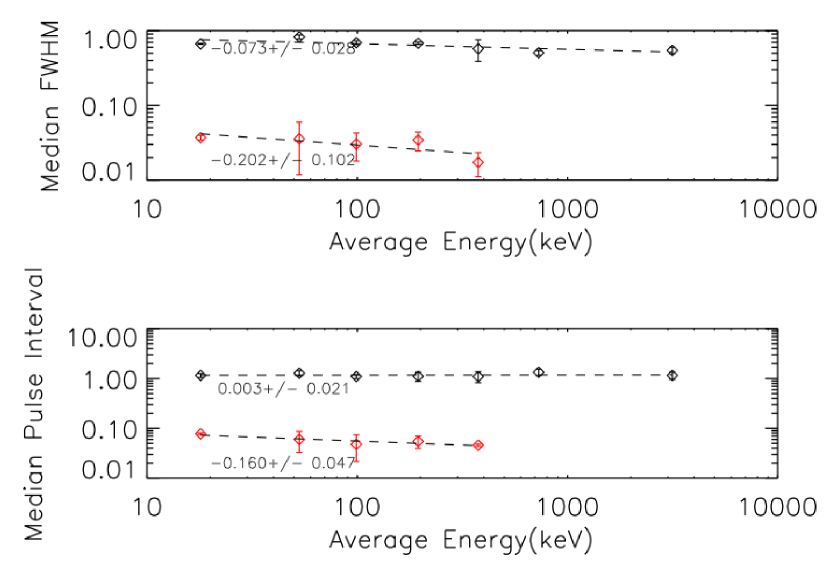
Figure 11: Evolution of the median pulse width (top) and median pulse intervals between sucessive pulses (bottom) for long and short GRBs with energy. The upper plot (in black) in each panel are the data for long bursts and the lower plot (in red) are for short bursts. In the case of short bursts both the pulse width and pulse interval show a faster decrease with increasing energy. In the case of long bursts on the other hand the pulse width shows a slower decrease with increasing energy than that for short bursts. The median pulse interval hardly seems to change with increasing energy in the case of long GRBs. The fitted power laws are shown as dotted lines for each type of GRBs and the fitted slopes are indicated.

Figure 10 shows the evolution of the distributions of time intervals between neighboring pulses of long and short bursts. Also shown are the best-fit lognormal functions in each energy band both for long and short GRBs. Figure 11 shows the variation of the median pulse width (FWHM) and median time interval between successive pulses as a function of increasing energy for long and short bursts. We note marked differences in the evolution of these 2 parameters for the two types of bursts. In both cases the short bursts show a relatively rapid decrease with energy as compared to long GRBs in agreement to earlier results where a general tendency of GRB pulses to be narrower at higher energies has been identified (Norris et al.,, 1996). The energy dependence of median pulse widths can be represented as $\Delta t\propto~{}E^{\alpha_{\rm w}}$ where $\alpha_{w}=0.07\pm 0.03$ for long bursts, while $\alpha_{\rm w}=-0.2\pm 0.1$ for short bursts. The median pulse interval also evolves very differently in the case of long and short bursts. Both show a power law dependence, with the exponents for long and short GRBs being $\alpha_{\Delta\rm t}=0.003\pm 0.02$ and $\alpha_{\Delta\rm t}=-0.16\pm 0.05$, respectively. The slope for long GRBs is consistent with zero, indicating that the median interval size is constant with energy, while the short GRB pulses are more closely spaced at higher energies.

5 Discussion

Sari & Piran (1997) argued that the observed temporal structure of a GRB reflects the activity of the central engine that generates it. According to the internal shock model, the GRB pulses are formed by the collisions among relativistic shells ejected by the central engine with a distribution of Lorentz factors (${\gamma_{e}}$). A GRB pulse shape depends on three time scales. The hydrodynamic time scale, $t_{dyn}$ (that determines the pulse rise time), the angular spreading time scale, $t_{ang}$ (that determines the pulse decay time), and the cooling time scale, $t_{rad}$ (which is usually much shorter than the other two and can be ignored) (Kobayashi, et al.,, 1997; Katz,, 1997; Fenimore $et~{}al$.,, 1996). Hence the measured pulse shape parameters have the potential to diagnose the pulse characteristics such as the bulk Lorentz factors, $\gamma_{e}$, shell radii and thicknesses (Kocevski et al.,, 2003).

Because of relativistic radiation-beaming only a small cone of opening angle ${\gamma_{e}}^{-1}$ is visible to the observer. The time difference between $\gamma-$rays emitted on-axis and off-axis constitutes the pulse decay. The off-axis $\gamma-$rays are delayed by $T_{ang}=\frac{R_{e}}{2{\gamma_{e}}^{2}}$, where $R_{e}$ is the typical radius characterizing the emission shell (Nakar,, 2007). The decay times of short GRBs are shorter than those of the long ones. Assuming an internal shock origin for both, we consider the possible implications of our observational results. If the curvatures of the emitting shells ($R_{e}$) are similar for both GRB types, then shorter decay times would imply that the $\gamma-$ray emitting shells of short bursts have significantly larger Lorentz factors. On the other hand if the Lorentz factors are similar then the radii of the emitting shells are smaller in short GRBs, implying a more compact central engine. Ackermann et al. (2010) compare the estimates of $\Gamma_{\rm min}$ (the bulk Lorentz factors) for two long and one short GRBs. These are 900, 1000 and 1218, respectively, possibly indicating (albeit with small number statistics) that the shell radii of short GRBs are significantly smaller.

According to Dermer and Menon, (2009) the GRB central engine releases energy at a fixed rate over a time scale $\Delta_{0}/c$, where $\Delta_{0}$ is a characteristic size scale of the engine. Assuming that the shortest time scale in GRB prompt emission is the shortest pulse width, we can estimate the length scale of the GRB central engine. Using the mean shortest FWHM of short and long GRBs, 0.016 s and 0.087 s, respectively, we find their corresponding length scales to be $4.8\times 10^{8}$ cm and $2.6\times 10^{9}$ cm, respectively in the observer frame. To convert these length scales to the source frame, we use the mean redshifts, $z=2.245,0.862$, of 151 long and 12 short Swift GRBs . These are $8\times 10^{8}$ cm and $2.6\times 10^{8}$ cm, respectively. According to the GRB standard model (Mészáros,, 2006) the above length scales agree with the saturation radius of the fireball ($\sim 10^{9-10}$ cm), $i.e.,$ the radius signifying the end of the acceleration phase and the beginning of the coasting phase of the Lorentz factor $\gamma_{e}$. Our results imply that the central engines of short GRBs seem to have a relatively smaller saturation radii.

We now estimate the rest frame radii of the shells, which give rise to the pulses. According to Dermer, (2004) the radius of the emission shell $R_{e}$ is given by:

$$R_{e}\approx\frac{2\gamma_{e}^{2}ct_{var}}{1+z}$$

where $t_{var}$ is the GRB light curve variability time scale. We substitute $t_{var}$ with the mean FWHM values of the GRB pulses (which are 0.9 and 0.06 s for long and short bursts respectively) and assuming a typical value for $\Gamma_{e}\approx 1000$, we find that the mean shell radii are $1.7\times 10^{16}$ cm and $1.9\times 10^{15}$ cm for long and short bursts, respectively. Zhao, Li and Bai, (2011) find shell radii for the long GRB 080916C that are slightly larger but comparable to the above mean value. Even larger prompt emission radii were inferred for other GRBs by different estimates (Kumar $et~{}al.$,, 2007; Racusin,, 2008). Our mean shell radii agree with the radial distances when the internal shock phase ($\sim 10^{14-15}$ cm) or the prompt emission starts (Mészáros,, 2006), possibly indicating that the beginning of the internal shock phase occurs earlier for short bursts.

If the individual pulses in the GRB light curves are indeed formed by the collision of shells with unequal Lorentz factors (Rees and Mészáros,, 1994; Nakar and Piran,, 2002) then shorter intervals between pulses (Figure 5) imply that the relativistic shells are more frequent. However, the longer intervals between successive pulses and durations of long GRBs indicate that the central engine shell ejection persists for longer times. In other words, the duration as well as the structure of the light curve are indeed related to the central engine activity.

Temporal analysis of long and short GRB light curves carried out here supports the general observation that the short bursts are temporally similar to long ones but compressed in time, which could be related to the nature of the central engine of the respective bursts.

6 Acknowledgments

The GBM project is supported by the German Bundesministerium f ur Wirtschaft und Technologie (BMWi) via the Deutsches Zentrum f ur Luft-und Raumfahrt (DLR) under the contract numbers 50 QV 0301 and 50 OG 0502.

AJvdH was supported by NASA grant NNH07ZDA001-GLAST.

SMB acknowledges support of the Union Marie Curie European Reintegration Grant within the 7th Program under contract number PERG04-GA-2008-239176.

SF acknowledges the support of the Irish Research Council for Science, Engineering and Technology, cofunded by Marie Curie Actions under FP7.

We also acknowledge the constructive comments and suggestions from the anaonymous referee which improved the quality of presentation.

Table 1: List of GRBs, chosen for the present analysis. Also listed are their durations (column 2) and the number of fitted pulses (column3)

Burst $\#$	Duration $T_{90}$ (s)	$\#$ of Fitted Pulses
Long GRBs
bn080723557	$58.37\pm 1.98$	29
bn080723985	$42.80\pm 0.66$	18
bn080807993	$19.07\pm 0.18$	16
bn080817161	$60.29\pm 0.47$	14
bn080825593	$20.99\pm 0.23$	20
bn080906212	$2.875\pm 0.77$	5
bn080916009	$62.98\pm 0.81$	32
bn080925775	$31.74\pm 3.17$	15
bn081009690	$176.2\pm 2.13$	5
bn081101532	$8.260\pm 0.90$	7
bn081110601	$17.34\pm 0.68$	2
bn081121858	$41.98\pm 8.51$	9
bn081122520	$23.30\pm 2.11$	6
bn081125496	$9.280\pm 0.61$	4
bn081129161	$62.66\pm 7.32$	2
bn081207680	$97.28\pm 2.35$	3
bn081215784	$5.570\pm 0.14$	10
bn081224887	$16.45\pm 1.16$	4
bn081231140	$28.74\pm 2.61$	3
bn090102122	$26.62\pm 0.81$	25
bn090131090	$35.07\pm 1.06$	8
bn090217206	$33.28\pm 0.72$	23
bn090323002	$135.2\pm 1.45$	17
bn090328401	$61.70\pm$ 1.81	7
bn090424592	$14.14\pm$ 0.26	15
bn090425377	$75.39\pm$ 2.45	3
bn090528516	$79.04\pm$ 1.09	16
bn090529564	$9.850\pm$ 0.18	7
bn090618353	$112.4\pm$ 1.09	20
bn090620400	$13.57\pm$ 0.72	5
bn090623107	$47.11\pm$ 2.57	18
bn090626189	$48.90\pm$ 2.83	24
Short GRBs
bn080905499	$0.960\pm$ 0.35	7
bn081209981	$0.192\pm$ 0.14	2
bn081216531	$0.768\pm$ 0.43	7
bn090227772	$1.280\pm$ 1.03	5
bn090228204	$0.448\pm$ 0.14	9
bn090305052	$1.856\pm$ 0.58	10
bn090308734	$1.664\pm$ 0.29	7
bn090429753	$0.640\pm$ 0.47	3
bn090510016	$0.960\pm$ 0.14	12
bn090617208	$0.192\pm$ 0.14	3

Table 2: The lower edges of the 8 energy channels used for pulse fitting of GRB light curves using the 2 types of GBM detectors. The upper energy edge of channel 7 is assumed to be twice the lower energy edge of that channel.

Channel $\#$	0	1	2	3	4	5	6	7
NaI (keV)	8.0	20	40	70	142	270	524	$>$985
BGO (MeV)	0.11	0.28	0.55	1.4	3.3	7.2	19.2	$>$45.5

Table 3: The variation of the number of fitted pulses in various NaI energy ranges for a sample of long bursts.

NaI Energy Range (keV)	8-20	20-40	40-70	70-142	142-270	270-524
Mean Energy (keV)	12.5	28.3	53.5	100.0	195.6	376.1
bn081207680	2	2	2	2	2	2
bn081215784	8	9	9	9	8	8
bn081231140	3	3	3	3	3	2
bn090217206	19	20	23	26	19	19
bn090323002	18	16	20	26	20	18
bn090328401	6	6	4	5	6	5
bn090424592	13	15	16	17	14	11
bn090529564	7	8	6	9	8	6
bn090618353	23	22	24	26	30	24
bn090626189	30	33	32	32	26	20

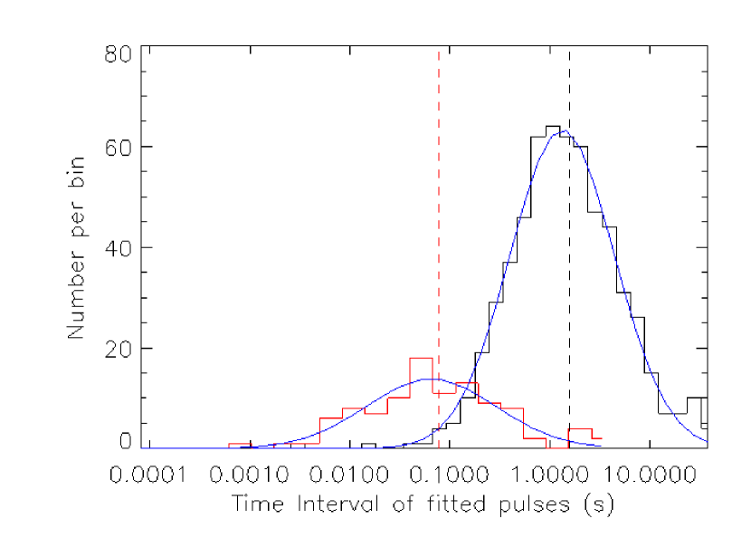
Figure 5: Distributions of the time intervals between successive pulses ($\Delta t$) for long (histogram shown in black) and short (histogram shown in red) bursts. A lognormal function is fitted to each of the distributions. The mean values of $\Delta t$ (from the fit) for long and short bursts are 1.53 s and 0.076 s and the standard deviations are 3.6 and 5.1 respectively. The vertical dashed lines indicate the median values of the time intervals between successive pulses for each class of GRBs.

References

- Aitchison and Brown, (1969) Aitchison, J. and Brown, J. A. C., 1969, “The Lognormal Distribution”, Cambridge University Press.
- Bissaldi,et al., (2011) Bissaldi,E. et al., 2011, ApJ, 733, 97
- Chiang, (1998) Chiang, J., 1998, ApJ, 508, 752.
- Daigne and Mochkovitch, (2003) Daigne, F. and Mochkovitch, R., 2003, MNRAS, 587, 592.
- Dermer and Mitman, (1999) Dermer, C. D. and Mitman, K. E., 1999, ApJ, 513, L5.
- Dermer, (2004) Dermer, C. D., 2004, ApJ, 614, 284.
- Dermer and Menon, (2009) Dermer, C. D. and Menon, G., “High Energy Radiation from Black Holes”, 2009, Princeton University Press.
- Eichler et al., (1989) Eichler, D., Livio, M., Piran, T. and Schramm, D. N., 1989, Nature, 340, 126
- Fenimore ., (1995) Fenimore, E., in’t Zand, J. J. M., Norris, J. P., Bonnell, Nemiroff, R. J., 1995, ApJ, L101
- Fenimore ., (1996) Fenimore, E., Madras, C. D. and Sergei, N., 1996, ApJ, 473, 998
- Fenimore et al., (1997) Fenimore, E., Ramirez-Ruiz, R. and Summer, M. C., 1997, Gamma-ray Bursts, 4th Huntsville Symposium, Ed. Meegan, C., Preece, R. and Koshut, T., AIP Conf. Proc., NY, 428, 657.
- Gehrels, (2005) Gehrels, N. et al., 2005, Nature, 437, 851.
- Gögüs et al., (2000) Gögüs, E., , 2000, ApJ, 532, L121.
- Guiriec, et al. (2010) Guiriec, S., et al., 2010, ApJ, 725, 225
- Gupta et al., (2000) Gupta, V., Dasgupta, P. and Bhat, P. N., 2000, Gamma-ray Bursts, 5th Huntsville Symposium, Ed. Kippen, R., Mallozzi, R. M. and Fishman, G. J., AIP Conf. Proc., NY, 526, 215.
- Hakkila and Cumbee, (2008) Hakkila, J. and Cumbee, R. S., 2008, Gamma-ray Bursts, 6th Huntsville Symposium, Ed. Meegan, C. A., Gehrels, N. and Kouveliotou, C., AIP Conf. Proc., NY, 1133, 379.
- Hakkila and Preece, (2011) Hakkila, J. and Preece, R. D., 2011, arXiv:1103.5434
- Horváth, (2002) Horváth, I., 2005, A&A, 392, 791.
- Hurley et al., (1994) Hurley K. J., McBreen B., Rabbette, M., Steel, S., 1994, A&A, 288, L49
- Ioka and Nakamura, (2002) Ioka, K and Nakamura, T., 2002, ApJ, 570, L21.
- Katz, (1997) Katz, J. I., 1997, ApJ, 490, 663
- Kobayashi, et al., (1997) Kobayashi, S., Piran, T. and Sari, R., 1997, ApJ, 490, 92
- Kouveliotou, et al., (1993) Kouveliotou, C., Meegan, C. A., Fishman, G. J., Bhat, N. P., Briggs, M. S., Koshut, T. M., Paciesas, W. S., and Pendleton, G. N., 1993, ApJ, 413, L101
- Kocevski et al., (2003) Kocevski, D., Ryde, F. and Liang, E., 2003, ApJ, 596, 389.
- Kumar , (2007) Kumar, P., 2007, MNRAS, 376, L57.
- Lee, Bloom and Petrosian, (2000) Lee, A., Bloom, E. D. and Petrosian, V., 2000, ApJS, 131, 1.
- Leo, (1994) Leo, W. R., “Techniques for Nuclear and Particle Physics Experiments” Springer-Verlag, 1994, pp190.
- Li and Fenimore, (1996) Li, H. and Fenimore, E., 1996, ApJ, 469, L115.
- McBreen et al., (1994) McBreen B., Hurley K. J., Long R., Metcalfe L., 1994, MNRAS, 271, 662.
- McBreen et al., (2001) McBreen S., Quilligan F., McBreen, B., Hanlon, L. and Watson, D., 2001, A&A, 380, L31.
- Meegan et al., (2009) Meegan, C. A., Lichti, G., Bhat, P. N., Bissaldi, E., Briggs, M. S., Connaughton, V., Diehl, R., Fishman, G., Greiner, J., Hoover, A. S., van der Horst, A. J., von Kienlin, A., Kippen, R. M., Kouveliotou, C., McBreen, S., Paciesas, W. S., Preece, R., Steinle, H., Wallace, M. S., Wilson, R. B., and Wilson-Hodge, C., 2009, ApJ, 702, 791
- Mészáros and Rees, (1993) Mészáros, P., and Rees, M. J., 1993, ApJ, 405, 278.
- Mészáros, (2006) Mészáros, P., 2006, Reports of Progress in Physics, 69, 2259.
- Nakar and Piran, (2002) Nakar, E. and Piran, T., 2002, ApJ, 572, L139.
- Nakar and Piran, (2002) Nakar, E. and Piran, T., 2002, MNRAS, 331, 40.
- Nakar, (2007) Nakar, E., 2007, Phys. reports, 442, 166.
- Narayan , (1992) Narayan, R., Paczynski, B. and Piran, T., 1992, ApJ, 395, L83
- Norris et al., (1996) Norris, J. P., Nemiroff, R. J., Bonnell, R. J., Scargle, J. D., Kouveliotou, C., Meegan, C. A., Fishman, G. J., 1996, ApJ, 459, 393.
- Norris et al., (2005) Norris, J. P., Bonnell, J. T., Scargle, J. D., Hakkila, J. and Giblin, T. W., 2005, ApJ, 627, 324.
- Paciesas, et al., (2011) Paciesas, W. S., et al., 2011, “The Fermi GBM Gamma-Ray Burst Catalog: The First Two Years” (in preparation)
- Preece, et al., (2000) Preece, R. D., et al., 2000, ApJS, 126, 19
- Quilligan et al., (2002) Quilligan F., McBreen, B., Hanlon, L., McBreen, S., Hurley, K. J. and Watson, D., 2002, A&A, 385, 377.
- Quilligan et al., (1999) Quilligan F., Hurley K. J., McBreen B., Hanlon L., Duggan P., 1999, A&AS, 138, 419.
- Racusin, (2008) Racusin, J. L., 2008, Nature, 455, 183.
- Ramirez and Fenimore, (2000) Ramirez-Ruiz, R. and Fenimore, E., 2000, ApJ, 539, 712.
- Rees and Mészáros, (1994) Rees, M. and Mészáros, P., 1994, ApJ, 430, L93.
- Sari and Piran, (1997) Sari, R. and Piran, T., ApJ, 485, 270.
- Woosley and Heger, (2006) Woosley, S. E. and Heger, A., 2006, ApJ, 637, 914
- Woosley and Bloom, (2006) Woosley, S. E. and Bloom, J. S. 2006, ARA&A, 44, 507
- Zhao, Li and Bai, (2011) Zhao, X., Li., Z. and Bai, J., 2011, ApJ, 726, 89