Multiscale magnetic fields in spiral galaxies: evolution and reversals

Abstract

Context. Magnetic fields in nearby, star-forming galaxies reveal large-scale patterns, as predicted by dynamo models, but also a variety of small-scale structures. In particular, a large-scale field reversal may exist in the Milky Way while no such reversals have been observed so far in external galaxies.

Aims. The effects of star-forming regions of galaxies need to be included when modelling the evolution of their magnetic fields, which can then be compared to future radio polarization observations. The conditions leading to large-scale field reversals also need clarification.

Methods. Our simplified model of field evolution in isolated disc galaxies includes a standard mean-field dynamo and continuous injection of turbulent fields (the effect of supernova explosions) in discrete star forming regions by implicit small-scale dynamo action. Synthetic maps of radio synchrotron emission and Faraday rotation measures are computed for galaxies at different evolutionary stages.

Results. A large-scale dynamo is essential to obtain regular large-scale spiral magnetic fields, as observed in many galaxies. These appear, on kpc scales in near energy equilibrium with the turbulence, after 1–2 Gyr (corresponding to redshift about $4-3$). The injection of turbulent fields generates small-scale field structures. Strong injected small-scale fields and a large dynamo number (e.g. rapid rotation) of a galaxy favour the generation of field reversals. Depending on the model parameters, large-scale field reversals may persist over many Gyrs and can survive until the present epoch. Significant polarized radio synchrotron emission from young galaxies is expected at redshift $\leq 4$. Faraday rotation measures (RM) are crucial to detect field reversals. Large-scale RM patterns of rotation measures can be observed at redshift $\leq 3$.

Conclusions. Our model can explain the general form of axisymmetric spiral fields with many local distortions, as observed in nearby galaxies. For a slightly different choice of parameters, large-scale field reversals can persist over the lifetime of a galaxy. Comparing our synthetic radio maps with future observations of distant galaxies with the planned Square Kilometre Array (SKA) and its precursors will allow testing and refinement of models of magnetic field evolution.

1 Introduction

Magnetic fields of nearby spiral galaxies have been investigated intensively since the 1980s. The strength and configuration of their large-scale components and the scale and strength of the small-scale magnetic field were addressed observationally, while dynamo theory provided models for their origin and evolution (see e.g. Beck et al. 1996, Widrow 2002 and Kulsrud & Zweibel 2008 for reviews). On the other hand, this view of the problem is constrained by the limited available sample of nearby spiral galaxies and does not address many problems which are important from the astrophysical viewpoint, for example the relation between galactic morphology (spiral arms, bars, halos, interactions) and the magnetic fields, or the occurrence of large-scale field reversals. Perhaps even more important is the problem of the magnetic field evolution in the first galaxies to form. This is the topic of this paper.

However, our knowledge concerning the details of hydrodynamics and magnetic fields in the earliest galaxies is very limited and substantially constrains the direct numerical simulations of the magnetic field evolution in these galaxies. This motivated Arshakian et al. (2009, 2011) to exploit simple semi-qualitative estimates taken from conventional galactic dynamo models to derive observational tests for magnetic fields in evolving galaxies.

The new generation of radio telescopes (under construction or under development) such as the Square Kilometre Array (SKA) and its precursors opens a broader perspective, that will enable a substantial enlargement of the variety of galaxies with known magnetic field configurations, and will address many points which have remained inaccessible up to now (Beck 2010). In particular, a natural idea here is to address theoretically magnetic fields in galaxies with as large redshifts as possible, in order to understand the magnetic field evolution in the earliest galaxies with the intention of observing them with the SKA (e.g. Murphy 2009). The key issue here is to suggest a set of observational tests for the first galaxies that lie within the capabilities of this new generation of telescopes.

Numerical simulations using several approaches have illuminated particular features of the magnetic field evolution during the course of galactic formation and evolution (e.g. Sur et al. 2007, Gressel et al. 2008, Hanasz et al. 2009, Wang & Abel 2009, Mantere et al. 2010, Schleicher et al. 2010, Kulpa-Dybel et al. 2011). Detailed models attempt to simulate a wide range of physical processes, and contain many governing parameters which need to be specified in order to describe a particular galaxy or a morphological type of galaxies. The complexity of parametric space and the huge processing times make an extensive inspection of their parameter space impractical.

The aim of this paper is to introduce a new type of mean-field galactic dynamo model which solves a relatively detailed set of mean-field dynamo equations coupled to the continuous injection of small-scale fields, and improves on the semi-qualitative estimates by Arshakian et al. (2009). On the other hand, our model is much simpler than those involving direct numerical simulations. The model also allows us to mimic to some extent the contribution of small-scale magnetic fields to the overall field configuration, in contrast to conventional mean-field dynamo models which take into account only the large-scale component. The relatively simple nature of our model makes a fairly detailed investigation of the parameter space a realistic proposition, and allows us to isolate robust features of the dynamo-generated magnetic fields which are suitable for observational identification. Future investigation of these results by more detailed models are highly welcome.

Our new model is situated between qualitative and semi-analytical estimates and direct numerical simulations. It is based on what has become known as the no-$z$ model, suggested by Subramanian & Mestel (1993) and Moss (1995, 1997). The idea is to average the magnetic fields in the galactic disc over various heights $z$ above and below the central galactic plane. This average becomes dependent on the galacto-centric radius $r$ and the azimuthal angle $\phi$ but is independent of the perpendicular coordinate $z$. The resulting 2D problem is then numerically affordable. As a seed field for the model we take a random seed field, and include continuous generation of small-scale random magnetic fields at the lowest scale resolvable by our numerical code (and similar to the seed field in strength and structure) during the galactic evolution. Then we link the dynamo and star-formation history to simulate the cosmological evolution of the magnetic structure.

Our model is based on a 2D set of dynamo equations which yields a 2D magnetic field configuration at the equatorial plane of a galaxy. Then we restore the vertical magnetic field component at this plane from the divergence-free condition and extrapolate the components from the equatorial plane to the whole disc. As a result we get a 3D model after explicit solution of 2D equations, which is computationally efficient.

Finally, from the magnetic field structures we simulate the expected total and polarized emission, and Faraday rotation measures (RMs) in these disc galaxies.

The main message obtained from the model can be summarized as follows. We recognize two phases of the evolution of galactic magnetic fields. Firstly, a large-scale magnetic field configuration develops from the random seed field. This stage is quite short and takes 1–2 Gyr. Secondly, the magnetic field becomes quite regular and close to an axisymmetric spiral structure, but affected by fluctuations. The main issue is that we obtain two different types of large-scale magnetic field configuration: (1) axisymmetric structures that have the same field direction over the whole galactic disc, (2) axisymmetric spiral fields that are restricted to two or even three separate intervals in radius (rings) with the field reversing direction between neighbouring rings.

2 A model for the evolution of magnetic fields in galaxies

A three-phase model for the evolution of magnetic fields in isolated (without merger) disc galaxies in the context of the hierarchical structure formation cosmology was developed by Arshakian et al. (2009). According to this model, in the first phase weak fields of order $\sim 10^{-18}$ G were generated by the Biermann battery mechanism and/or the Weibel instability in the first dark matter halos. The second phase was manifested by merging of halos and thermal virialization of protogalaxies. During this epoch the small-scale dynamo was able to amplify effectively the turbulent magnetic field up to the energy level of equilibrium with turbulent kinetic energy ($\sim 10^{-5}$ G) in a relatively short timescale of a few hundreds of million years. The third phase started at the epoch of disc formation (at a redshift of about 10) that occurred by dissipation of the protogalactic halo. The magnetic field preserved in the protogalactic halo served as a seed field in the disc ($\sim 10^{-7}$ G), which was further amplified by the mean-field dynamo to the equipartition level ($\sim 10^{-5}$ G) in few Gyrs and ordered on scales of up to galactic scale in about 13 Gyr, this stage lasting until the present epoch. In semi-analytical models of the evolution of regular magnetic fields Arshakian et al. (2011) proposed that the configuration of the initial regular field in the third phase was “spotty” over the galactic disc. The differential rotation initially stretches the magnetic spots in the azimuthal direction as they appear, and field reversals can be formed in few Gyrs by the effects of the large-scale dynamo action, and eventually an axisymmetric field similar to that of many present-day galaxies.

In this section, we adopt some of the ideas of the semi-analytical model of Arshakian et al. (2009, 2011) and develop an evolutionary model of a disc galaxy (phase 3), based on explicit solutions of the dynamo equations coupled to the star formation rate.

2.1 Star-formation and gas turbulence in the disc

The variations of the star-formation rate (SFR) and the physical/geometrical parameters of the disc drive the evolution of regular magnetic fields in galaxies (Arshakian et al. 2011). Star formation can be triggered by different processes including, for example, gravitational instability, and the interaction of clouds and tidal forces in isolated and merging galaxies (Kennicutt et al. 1987; Combes 2005). The rate of SN explosions is proportional to the SFR. Supernova remnants (SNRs) drive the turbulence of the interstellar medium (ISM) and determine the characteristic velocity dispersion of the gas, characterized by the turbulent velocity $v$. The latter is known to be correlated with SFR for nearby galaxies (Dib et al. 1996); it is almost constant for low SFRs (up to SFR values typical of the Milky Way) with $v\approx 10$ km s^-1 and grows exponentially at higher SFRs as typical for starburst galaxies. Star formation in isolated, young galaxies is more efficient because more gas is available at high redshifts (redshift $\sim 1.3$, Ryan et al. 2007). SFR is proportional to the gas mass density (the Kennicutt-Schmidt law) and, hence, the SFR history of disc galaxies is different for galaxies with different Hubble types. Modelling of SFR indicates that a constant SFR is appropriate for late-type spirals (Sd) while the SFR decreases with galaxy age for earlier types (Sc, Sb, and Sa; Sandage 1986, Kotulla et al. 2009). For simplicity, we consider an evolving Milky Way-type galaxy with constant SFR of 1 $M_{\sun}\,{\mathrm{yr}^{-1}}$ and constant turbulent velocity, $v=10$ km s^-1 throughout its evolution.

Star formation generates supernova explosions which are the main source of turbulence in the galaxy disc and in turn inject small-scale magnetic fields. In our model the field injection occurs at regular time intervals simultaneously at a number of random locations with a volume filling factor of about 1%.

2.2 The dynamo model

We use a thin disc galaxy code with the ”no-$z$” formulation (e.g. Subramanian & Mestel 1993; Moss 1995 and subsequent papers), taking the $\alpha\omega$ approximation. This code solves explicitly for the field components parallel to the disc plane with the implicit understanding that the component perpendicular to this plane (i.e. in the $z$-direction) is given by the condition $\nabla\cdot{\bf B}=0$, and that the field has even (quadrupole-like) parity with respect to the disc plane. The field components parallel to the plane can be considered as mid-plane values, or as a form of vertical average through the disc (see, e.g., Moss 1995). The key parameters are the aspect ratio $\lambda=h/R$, where $h$ corresponds to the semi-thickness of the warm gas disc and $R$ is its radius, and the dynamo numbers $R_{\alpha}=\alpha_{0}R/\eta,R_{\omega}=\Omega_{0}R^{2}/\eta$. $\lambda$ must be a small parameter. $\eta$ is the turbulent diffusivity, assumed uniform, and $\alpha_{0},\Omega_{0}$ are typical values of the $\alpha$-coefficient and angular velocity respectively. Thus the dynamo equations become in cylindrical polar coordinates $(r,\phi,z)$

$$\frac{\partial B_{r}}{\partial t} = -R_{\alpha}B_{\phi}-\frac{\pi^{2}}{4}B_{r}$$ (1)

$$+\lambda^{2}\left(\frac{\partial}{\partial r}\left[\frac{1}{r}\frac{\partial}{\partial r}(rB_{r})\right]+\frac{1}{r^{2}}\frac{\partial^{2}B_{r}}{\partial\phi^{2}}-\frac{2}{r^{2}}\frac{\partial B_{\phi}}{\partial\phi}\right),$$

$$\frac{\partial B_{\phi}}{\partial t} = R_{\omega}rB_{r}\frac{d\Omega}{dr}-R_{\omega}\Omega\frac{\partial B_{\phi}}{\partial\phi}-\frac{\pi^{2}}{4}B_{\phi}$$ (2)

$$+\lambda^{2}\left(\frac{\partial}{\partial r}\left[\frac{1}{r}\frac{\partial}{\partial r}(rB_{\phi})\right]+\frac{1}{r^{2}}\frac{B_{\phi}^{2}}{\partial\phi^{2}}-\frac{2}{r^{2}}\frac{\partial B_{r}}{\partial\phi}\right),$$

where $z$ does not appear explicitly. This equation has been calibrated by introduction of the factors $\pi^{2}/4$ in the vertical diffusion terms. Of course, in principle in the $\alpha\omega$ approximation the parameters $R_{\alpha},R_{\omega}$ can be combined into a single dynamo number $D=R_{\alpha}R_{\omega}$, but for reasons of convenience and clarity of interpretation we choose to keep them separate.

In the current implementation the code is now written in cartesian coordinates $x,y,z$, with $z$-axis parallel to the rotation axis. Length, time and magnetic field are non-dimensionalized in units of $R$, $h^{2}/\eta$ and the equipartition field strength $B_{\rm eq}$ respectively.

A naive algebraic $\alpha$-quenching nonlinearity is assumed, $\alpha=\alpha_{0}/(1+B^{2}/B_{\rm eq}^{2})$, where $B_{\rm eq}$ is the strength of the equipartition field in the general disc environment, not necessarily that in the “spots” – see below. We appreciate that more sophisticated approaches to the saturation process exist, and that careful consideration of helicity transport processes is required to demonstrate that limitation of the large-scale field at very low levels (”catastrophic quenching”) does not occur – see e.g. Vishniac & Cho (2001), Kleeorin et al. (2002, 2003), Sur et al. (2007). However it does appear that in some cases at least, such a naive algebraic quenching can reproduce reasonably well the results from a more sophisticated treatment (e.g. Kleeorin et al. 2002). Of course, more sophisticated forms of algebraic alpha-quenching are also possible, such as forms that are non-local in space or time. We choose to use the simplest possible approach.

In order to implement boundary conditions that ${\bf B}\rightarrow{\bf 0}$ at the disc boundary (as used in earlier versions of the code written in polar coordinates), the disc region $x^{2}+y^{2}\leq 1$ was embedded in a larger computational region $|x|\leq x_{\rm b},|y|\leq y_{\rm b}$, where $x_{\rm b}=y_{\rm b}\approx 1.35$. In the region $x^{2}+y^{2}>1$ outside of the disc the field satisfies the diffusion equation without dynamo terms. This was found to give solutions that were small at the disc boundary, and rapidly became negligible outside of the disc. The standard implementation used a uniform grid of $229\times 229$ points over $-1\leq x,y\leq+1$, with appropriate additional points in the surrounding ”buffer zone”. With a nominal galaxy radius of 10 kpc, this gives a resolution of about 88 pc. With $R=10$ kpc, the assumed disc semi-thickness of $h=500$ pc gives $\lambda=0.05$, and the unit of time is then approximately 0.78 Gyr. Subsequently, all fields are in units of the equipartition field $B_{\rm eq}$ (i.e. energy equipartition with turbulence), unless explicitly stated.

The coefficient $\alpha_{0}$ is assumed to be uniform in the work described in this paper. We performed tests with a radially varying coefficient $\alpha_{0}=\alpha_{0}(r)$, but this did not change our results significantly.

Taking typical galactic values, we can estimate $R_{\alpha}=O(1)$, $R_{\omega}=O(10)$ (i.e. $D\approx 10$). However, a considerable degree of uncertainty is attached to the conventional estimate $\eta=10^{26}$ cm² s^-1, and correspondingly to $R_{\alpha}$ and $R_{\omega}$.

¿From experiments with an arbitrary seed field, the marginal values are $R_{\alpha}\approx 0.6$ with $R_{\omega}=8$, so the critical dynamo number for this no-$z$ model is $D_{\rm cr}\approx 5$. This value can be compared with the critical dynamo number $D_{\rm cr}\approx 7$ which comes from the local disc dynamo problem (Ruzmaikin et al. 1988) and illustrates the degree of consistency between the local and no-$z$ models. In any case, the above estimates of $R_{\alpha}$ and $R_{\omega}$ correspond to a somewhat supercritical dynamo.

Of course these estimates apply to conditions in contemporary spiral galaxies and may need revision for very young objects – we will return to this later in Sect. 5. Note again that we use $z$ as a cartesian coordinate, and not as redshift (except in one instance, where explicitly stated.)

2.3 The field injection algorithm

In our attempt to describe the generation of small-scale fields in star-forming regions, $n_{\rm sp}$ spot centres $(x_{\rm sp},y_{\rm sp})$ are generated at random positions within the disc ($r\leq 1$). These rotate with the local angular velocity. At time intervals $dt_{\rm inj}$ a random field $B_{\rm x,sp},B_{\rm y,sp}$ is assigned to each of these positions $(x_{\rm sp},y_{\rm sp})$. We, slightly arbitrarily, take $dt_{\rm inj}$ to be about 10 million years. The neighbouring points, out to a radius $3\,r_{\rm sp}$, are assigned non-zero magnetic field by assuming a Gaussian distribution of components $B_{\rm x},B_{\rm y}$ with half-width $r_{\rm sp}$ and central values $B_{\rm x,sp},B_{\rm y,sp}$. These spots are assumed to live for a time $dt_{\rm sp}>>dt_{\rm inj}$. After this time, the old spots disappear, and a new set of $n_{\rm sp}$ spots is generated using the above algorithm. The central field strength in each spot, $(B_{\rm x,sp}^{2}+B_{\rm y,sp}^{2})^{-1}$, is taken from a Gaussian distribution with central value $B_{\rm inj}$. Note that after injection, these fields undergo evolution and take part in the large-scale dynamo action: thus they are a sort of continually renewed seed field. Thus the process is not equivalent to evolving a conventional mean-field dynamo, giving a smooth, large-scale field, and then adding a random field component. For simplicity, all spots die, and are born, simultaneously.

A typical configuration of the initial field is shown in Fig. 1. For clarity, this figure plots $\@vec{B}$ vectors at only the central point of each spot. Note that we consider here magnetic field generation from a small-scale seed field and use a small-scale initial field that is random, and distributed in discrete patches. This seed is supplemented continually by the injection process. We stress that in many numerical simulations, a small-scale (e.g. Hanasz et al. 2009) or large-scale seed field, of dipolar or quadrupolar form is assumed. Such an initial condition makes implicit assumptions about the history of the field present as the galaxy forms. We take a somewhat different viewpoint.

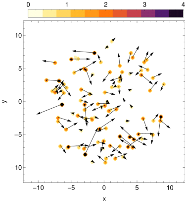
Figure 1: A typical configuration of the initial magnetic field; only the ${\@vec{B}}$ vectors at the centre of the spots are shown.

2.4 Model assumptions

The initial seed field is assigned by a run of the field injection algorithm, as described in Sect. 2.3, i.e. there is a random, spatially intermittent, initial field. The strength of this initial field (and also that of the fields subsequently injected) is determined by the parameter $B_{\rm inj}$ – see Sect. 2.3. Note that because we assume these fields to result from small-scale dynamo action in the spots ($\sim$ star-forming regions), their strength is near equipartition i.e. $B_{\rm inj}=O(1)$. In this preliminary study, there is no spatial weighting of the spot distribution process (Sect. 2.3), or $B_{\rm inj}$, nor any time dependence of $B_{\rm inj}$ or $n_{\rm sp}$. These assumptions correspond to a star formation history that is spatially and temporally uniform. Clearly a time and/or space dependence of the injection process could be introduced in further work.

The Gaussian half-width of the spots $r_{\rm sp}=0.01$ (=$100$ pc for R=$10$ kpc) gives an estimate for their filling factor $n_{\rm sp}r_{\rm sp}$ = $1\%$ for our standard model with $n_{\rm sp}=100$.

Throughout the paper we take a disc aspect ratio $\lambda=0.05$, and with a radius of $10$ kpc the disc semi-thickness is $500$ pc. For the rotation curve we take

$$r\frac{d\Omega}{dr}=\Omega_{0}\left(-\frac{1}{rR_{\rm gal}}\tanh(\frac{rR_{\rm gal}}{r_{0}})+\frac{1}{r_{0}\cosh^{2}(rR_{\rm gal}/r_{0})}\right),$$ (3)

where $r_{0}$ corresponds to the turnover radius for the rotational velocity. We take $r_{0}=0.2$ and show the dependence of azimuthal velocity on radius in Fig. 2.

Figure 2: The dependence of the scaled rotation velocity on radius for turnover radius $r_{0}=0.2$. We choose parameters so that the flat part of the rotation curve has $V_{\rm rot}\approx 200$ km s^-1, and $r=1$ corresponds to the dimensional radius 10 kpc.

3 The evolution of magnetic field in selected cases

We take initial conditions as described above and evolve Eqs. (1) and (2) until the time $t=17$, corresponding to a galaxy age $T=13.2$ Gyr since the epoch at redshift 10. We take this time $t=17$ as corresponding to the present day epoch. We made numerous runs with varying parameters. In order to constrain the number of free parameters, we keep $R_{\alpha}=1$ for most of our investigations, and discuss below the effects of changing $R_{\omega}$, $B_{\rm inj}$ and $n_{\rm sp}$. We also briefly mention at the end of Sect. 3.1 some effects of changes in $R_{\alpha}$.

3.1 The effects of varying the dynamo numbers

We discuss two models in some detail. They each have the standard parameters governing field injection as discussed above, and have $R_{\alpha}=1$, $B_{\rm inj}=1$. The first has $R_{\omega}=10$ (referred to as Model 138), and the field at galaxy age $T=13.2$ Gyr (present epoch) is seen to have no large-scale reversals – its evolution is shown in Fig. 3. The second example has $R_{\omega}=20$ (Model 135), and large-scale field reversals are visible from $T=2$ Gyr to $T=13$ Gyr – see Fig. 4. In Fig. 5 we show contours of the azimuthal field smoothed by a Gaussian filter of 100 pc half-width at $T=13.2$ Gyr, which illustrate clearly where large-scale reversals occur. In Fig. 3, panel (c) ($T=13.2$ Gyr), local reversals are visible near radius $r=0.85$ ($x\approx-0.5,y\approx 0.7$, $x\approx 0.3,y\approx 0.8$), which disappear with smoothing to 100 pc. Similar features can be found comparing the last panel of Fig. 4 with Fig. 5b. Other field configurations (with, say, a different number and position of reversals) are possible, depending on the dynamo parameters and the details of the field injection process, and we return briefly to this topic later.

(a)
(b)
(c)

Figure 3: Field vectors at galaxy ages $T=0.23,0.78$ Gyr (row (a)), $T=2.3,3.9$ Gyr (row (b)), and $T=7.8,13.2$ Gyr (row (c)), for the model with $R_{\omega}=10,R_{\alpha}=1,B_{\rm inj}=1$. The vectors give the magnetic field direction, their lengths are proportional to the magnetic field strengths. There are no large-scale reversals of field direction visible at the present day ($t=17$). In this and other plots, the axes are labeled in units of fractional galactic radius. (Model 138)

(a)
(b)
(c)

Figure 4: Field vectors at galaxy ages $T=0.23,0.78$ Gyr (row (a)), $T=2.3,3.9$ Gyr (row (b)), and $T=7.8,13.2$ Gyr (row (c)), for the model with $R_{\omega}=20,R_{\alpha}=1,B_{\rm inj}=1$. The vectors again give the magnetic field direction, their lengths are proportional to the magnetic filed strengths. There is one large-scale reversal visible at the present day ($T=13.2$ Gyr). (Model 135)

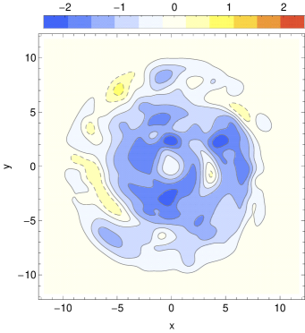
(a) (b)

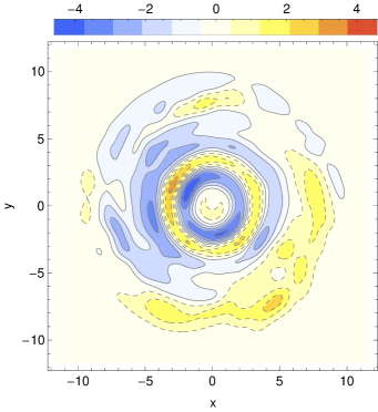
Figure 5: Contours of azimuthal field (in units of $B_{\rm eq}$), smoothed by a Gaussian filter of half-width 100 pc, at galaxy age $T=13.2$ Gyr. Positive values (clockwise rotation) are indicated by continuous contours, negative values (counterclockwise rotation) by broken contours. (a) $B_{\rm inj}=1,R_{\omega}=10$, (b) $B_{\rm inj}=1,R_{\omega}=20$.

Typical energy spectra are shown in Fig. 6 at several times. The energy in the large-scale field ($k<5$) can be seen to increase with time, while that with $k>5$ decreases. Model 135 shows an irregular distribution of energy in spectral space and large fluctuations in time. The ratio of small to large-scale magnetic field remains small, and decreases with time – see Fig. 7. In order to construct realistic synthetic polarization maps it is necessary to complete the simulated magnetic field by addition of an artificial turbulent contribution. This is discussed in Sect. 4.

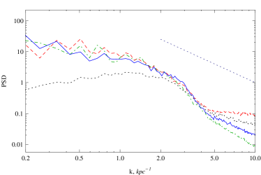
Figure 6: Energy spectral density at time $t=0.3$ (dotted), $t=3$ (dot-dashed), $t=10$ (dashed) and $t=17$ (solid). Upper panel: $B_{\rm inj}=1,R_{\omega}=10$ (Model 138) , lower panel: $B_{\rm inj}=1,R_{\omega}=20$ (Model 135). The broken line has slope $k^{-2}$.

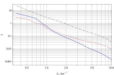
Figure 7: Ratio of small to large-scale magnetic energies $\lambda=\langle B(k>k_{s})\rangle/\langle B(k\leq k_{s})\rangle$ vs scale separation parameter $\lambda$ at time $t=0.3$ (dot-dashed), $t=10$ (dashed) and $t=17$: above - $B_{\rm inj}=1,R_{\omega}=10$ , below $B_{\rm inj}=1,R_{\omega}=20$.

An important result is that by the galaxy age $T=0.78$ Gyr (Figs. 3 and 4), a field of strength $B_{\rm eq}$ with a scale of several kpc is already present. This is a more-or-less inevitable result of the initially strong small-scale fields being stretched by differential rotation and then organized by the large-scale dynamo. We did also make a cursory investigation of the effect of changes in $R_{\alpha}$. Specifically, we looked at cases with $B_{\rm inj}=1$, with $R_{\omega}=10$, $R_{\alpha}=2$ and $R_{\omega}=20$, $R_{\alpha}=0.5$, i.e. the cases shown in Figs. 3 and  4 with increased/decreased $R_{\alpha}$, respectively. The magnetic field geometry is less sensitive to this parameter, and the effect of these changes on field geometry is minor. Increasing $R_{\alpha}$ in the first case increases the regularity of the field at $T=$17  $13.2$ Gyr ($t=17$), and removes any local reversals present. In the second case, the changes were almost indiscernable. The global energy varies slightly as the change in $R_{\alpha}$.

3.2 The effects of varying the field injection parameters

In order to demonstrate the roles of the parameters $n_{\rm sp}$ and $B_{\rm inj}$, we show in Fig. 8 the field configurations at $t=17$ (corresponding to an age of approximately 13.2 Gyr) for models with $R_{\alpha}=1,R_{\omega}=10$ and $B_{\rm inj}=1,2,4$ (i.e., increasing $B_{\rm inj}$ from the value used in the models described in Sect. 3.1).

Reducing the value of $n_{\rm sp}$ to 50 reduces the amount of disorder in the field (compare the last panel of Fig. 3 with panel (a) of Fig. 8). As less small-scale field is being injected, this is perhaps not so surprising.

We also now consider cases in which the turbulence in the star-forming regions (spots) is assumed to be significantly stronger than in the general ISM, giving an injected field larger than the general equipartition field, i.e. $B_{\rm inj}>1$. Note that we do not change the alpha-quenching formalism or the value of $B_{\rm inj}$ in the spots when $B_{\rm inj}>1$, as the dominant dynamo mechanism in the spots is assumed to be a small-scale dynamo to which we cannot apply the alpha-quenching concept. Moreover the filling factor of the high field region of the spots is small, and the usual $\alpha\omega$ dynamo operates through nearly all the disc. These assumptions are strongly supported by an experiment (not shown) where with the parameters of panel (c) of Fig. 8, a global alpha-quenching $\alpha=\alpha_{0}/(1+E)$, with $E$ a measure of the mean magnetic energy over the disc, was used. The resulting field vectors were very similar to those shown in panel (c) of Fig. 8. As $B_{\rm inj}$ increases, obviously does the disorder: compare panels (a), (b), (c) of Fig. 8. Further, the reduction of $n_{\rm sp}$ seems to produce some overall change to the field structure. Specifically, the reduced value of $n_{\rm sp}$ means, quite predictably, that for given $B_{\rm inj}$ the field is less disordered. Less predictably, perhaps, even when $B_{\rm inj}$ is increased and more disorder is apparent, the spiral structure is better defined and rather more open, until $B_{\rm inj}=4$, see the successive panels of Fig. 8.

(a) (b)

(c)

Figure 8: To illustrate the effects of changing the parameters $B_{\rm inj}$ and $n_{\rm sp}$. $B$-vectors at $T=13.2$ Gyr for models with $R_{\omega}=10,R_{\alpha}=1$, $n_{\rm sp}=50$ (cfed 100 normally); (a) $B_{\rm inj}=1$, (b) $B_{\rm inj}=2$, (c) $B_{\rm inj}=4$.

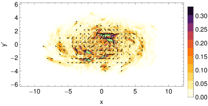
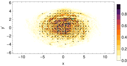
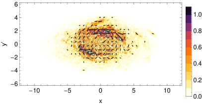
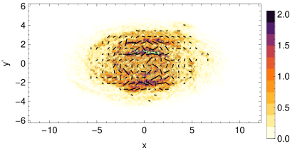
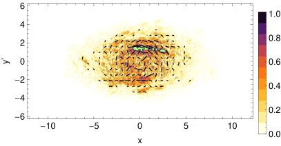
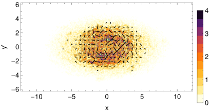
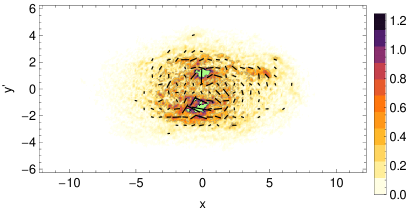
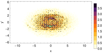
Figure 9: Models 138 ($R_{\omega}=10$, left), 135 ($R_{\omega}=20$, right): polarized synchrotron intensity (arbitrary units) at wavelength 21 cm, as seen in the frame of the galaxy. Top to bottom: $T=0.23$, $T=2.3$, $T=7.8$, $T=13.2$ Gyr. The small bars show the (unsigned) field directions.

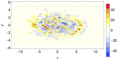
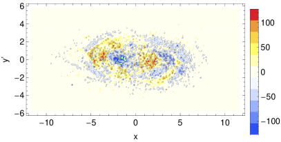
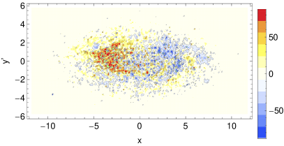
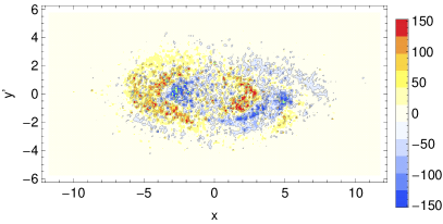
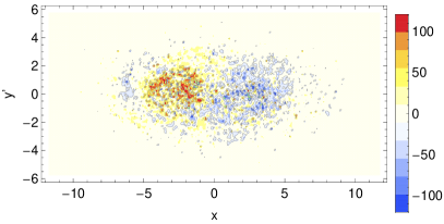
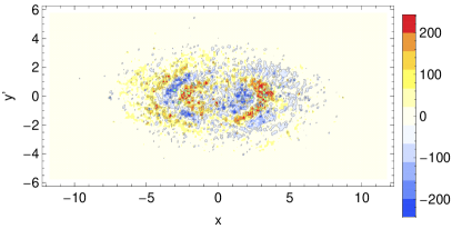
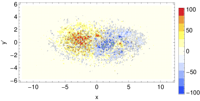
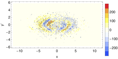
Figure 10: Models 138 (left), 135 (right): Faraday rotation measures (in $\rm rad/m^{2}$ assuming $B_{\rm eq}$=1 $\mu G$) at wavelength 21 cm, as seen in the frame of the galaxy. Top to bottom: $T=0.23$, $T=2.3$, $T=7.8$, $T=13.2$ Gyr.

4 Simulations of regular magnetic fields, total intensity, polarization and Faraday rotation of evolving galaxies

In order to construct an extension of the 2D magnetic field ${\mathbf{B}}(x,y)$ of our models to a 3D distribution ${\mathbf{B}}(x,y,z)$ in a galactic disc, use of a Fourier transform technique seems natural. We adopt the approach of writing the horizontal magnetic field in factorized form as

$$\hat{B}_{x}(k_{x},k_{y},k_{z})=\hat{B}_{x}(k_{x},k_{y})\hat{g}(k_{z}a_{h}),$$ (4)

$$\hat{B}_{y}(k_{x},k_{y},k_{z})=\hat{B}_{y}(k_{x},k_{y})\hat{g}(k_{z}a_{h}),$$ (5)

$$g(z)=\exp(-z^{2}),$$ (6)

where $(\hat{.})$ denotes the Fourier transform, ${\mathbf{k}}$ is the wave vector and $a_{h}$ is a vertical scale. The structures in the horizontal plane are extrapolated in height with the same scales as the associated horizontal structure, $a_{h}=(k_{x}^{2}+k_{y}^{2})^{-1/2}$. We limit $a_{h}$ by the galactic scale height $h_{g}=2$ kpc. The solenoidal condition allows the computation of the vertical magnetic field component

$$\hat{B}_{z}(k_{x},k_{y},k_{z})=-\frac{\hat{B}_{x}(k_{x},k_{y},k_{z})k_{x}+\hat{B}_{y}(k_{x},k_{y},k_{z})k_{y}}{k_{z}}.$$ (7)

The turbulent component of magnetic field in the whole galactic disc is evaluated in the same manner as suggested by Arshakian et al. (2011). The thermal electron distribution is assumed as

$$n_{e}(r,z)=n_{0}\exp{\left[-\left(\frac{r}{r_{0}}\right)^{2}\right]}\exp{\left[-\left(\frac{z}{h_{0}}\right)^{2}\right]},$$ (8)

where exponential scales are $r_{0}=5h_{0}=5.9$ kpc and $n_{0}=0.03$ $\rm cm^{-3}$. The cosmic-ray density has the same shape but measured in an arbitrary units. The synchrotron spectral index is 0.8.

The time evolution of the total and polarized synchrotron intensity and RM in the rest frame of the galaxy inclined at 60 degrees for the models 138 and 135 is shown in Figs. 9 and 10 as a series of snapshots. Here we take $B_{\rm eq}=1\mu{\rm G}$.

Polarized emission is detected already in the early phases of galaxy evolution around galaxy age $T=0.23$ Gyr, corresponding to redshift $\approx 7.5$ (Fig. 9, first row), but the intensity is still low. The equipartition level is reached around $T=1$ Gyr (redshift $\approx 4$), so that strong emission is seen after $T=2.3$ Gyr (Fig. 9, rows 2–4). The two models show different distributions of the polarized emission across the galaxy, but these will depend slightly on the choice of the initial parameters. The occurrence of large-scale field reversals, the main difference between the models with different choice of the dynamo number $R_{\omega}$, cannot be distinguished from Fig. 9 because polarized emission is not sensitive to field reversals.

Faraday rotation measures (RM) (Fig. 10) clearly show the development of field reversals with galaxy age. At early times, RM is significant in restricted areas. Large-scale RM patterns are seen after age $T\approx 2$ Gyr (redshift $\leq 3$), in excellent agreement with the estimate given by Arshakian et al. (2009). The main result of the improved model of this paper is the occurrence of large-scale reversals of Model 135 (Fig. 10, right column), which remain clearly visible until the present epoch.

Note that the polarized intensity and RM values in Figs. 9 and 10 refer to the galaxy frame. These maps will look different in the rest frame of the observer because of a frequency shift. Highly redshifted galaxies emit at high frequencies at which the depolarization effects are different: depolarization becomes weaker with increasing frequency. Weak regular magnetic fields at high redshifts and strong dilution of RM by a factor of $(1+{\sf z})^{-2}$ (here $\sf z$ is redshift) lead to small observable RM for distant galaxies. The effect of depolarization for polarized intensity and RM maps is discussed in Arshakian et al. (2011). Detection of RM patterns from distant galaxies will become possible only for large forthcoming radio telescopes such as the SKA.

5 Discussion

We can identify two stages in the development of the magnetic field from the random seed field to a mature magnetic field configuration. In the first stage the magnetic field has a spatially intermittent structure, whilst in the second the mature magnetic field has a regular structure with a large-scale component which is an almost axisymmetric spiral. The transition time from the first to the second stage is quite robust and depends on the diffusion time $t_{d}$ of the magnetic field through the vertical extent of the galactic disc ($t/t_{d}\approx 2$) which corresponds to 1–2 Gyr in dimensional units. If we assume that the galactic disc was formed at redshift around $10$, the transition to the mature field occurs at redshift $\approx 4-3$, which is too early to be observed even by the SKA. If however a galactic encounter or strong interaction ’resets the clock’, and so can be considered as the starting point for the field evolution, observation of a spotty field configuration or of a large number of reversals appears a realistic possibility.

The SKA will be able to recognize the regular field structures of nearby galaxies from RMs of background polarized sources behind a galaxy and continuous RM map of the diffuse polarized emission of a galaxy (Stepanov et al. 2008). The former approach will allow the simple field structures to be recognized at a distance of about 100 Mpc in disc galaxies having a size of $20$ kpc. With SKA angular resolution of 1 arcsec at 1.4 GHz, mapping of the diffuse emission of a galaxy itself can resolve RM patterns up to a distance $z\approx 0.11$, which corresponds to a comoving radial distance of $\approx 450$ Mpc.

We also learn from this work that the magnetic field evolution continues slowly over a very long time after a mature field configuration first appears. This evolution affects the size and exact location of the radial range (“ring”) filled with a spiral field of a given direction with respect to azimuth.

We also considered purely regular initial seed fields and also weak random initial seed fields with no injection, and confirmed that both evolve into smooth large-scale fields.

What is quite new and unexpected is the possibility to obtain several (two or even three) rings of oppositely directed magnetic fields in neighbouring rings and hence global field reversals between $T\approx 3$ Gyr and 13 Gyr. Global field reversals are not observed yet in nearby external galaxies. A reversal of several kpc extent in azimuth has been found between the Orion and Sagittarius arms in the Milky Way from pulsar RM data (e.g. Frick et al. 2001, Noutsos et al. 2008, Nota & Katgert 2010, Van Eck et al. 2011). Another possible reversal between the Orion and Perseus arms is difficult to prove or disprove with the data currently available (see Frick et al. 2001). Han et al. (2006) claimed that many magnetic field reversals can be recognized in the Milky Way. However, the existence of multiple reversals is not statistically well established (Men et al. 2008). The global field structure of the Milky Way it is not known yet.

Standard galactic dynamo models which start from a very week seed field give usually a final magnetic field configuration without reversals. Traditional mean-field dynamo theory has considered reversals as long-lived transients (Vasil’yeva et al. 1994, Moss et al. 1998, 2000, Petrov et al., 2001, 2002) which occur if the initial field is strong enough and has a suitable configuration. These traditional 1D models are however obviously too oversimplified to be fully convincing because they assume inter alia that the galactic magnetic field is purely axisymmetric. Here we consider a 2D model where the magnetic field can have an arbitrary configuration. We consider the results obtained in this paper to be sufficiently detailed to produce reliable results on the occurrence of reversals.

The strongly nonlinear initial conditions of our models (with field strengths of order the equipartition strength, even though with a small volume filling factor and no large-scale order) play a key role in determining the long-term evolution and structure of the magnetic field. Unlike conventional dynamo models, which begin with a weak seed field often of large scale, with no further intervention, the saturated state is now not solely determined by the dynamo parameters and the galaxy structure: the presence and nature of the small-scale magnetic field injections, especially that at $T=0$ is crucial. However, the dynamo number $R_{\alpha}R_{\omega}$ is also important: We show in Figs. 3 and 4 the differing field geometries obtained when $R_{\omega}$ is doubled. In the first case there are no large-scale field reversals at $T=13.2$ Gyr, but in the second a large-scale reversal is present. We found other models with two reversals present. Briefly, a larger dynamo number and a larger value of $B_{\rm inj}$ favor the presence of field reversals, cf. Figs. 3, 4 and 8. We intend to discuss this interesting aspect of the solutions in more detail in a separate paper (Moss & Sokoloff, in prep.).

We stress that a relatively small variation of the dynamo-governing parameters converts a model without global field reversals into a model with one or several global reversals. One important parameter turns out to be the dimensionless number $R_{\omega}$ which is determined by the angular rotation velocity, the galaxy size and the turbulent diffusivity. Faster galactic rotation tends to a larger value of $R_{\omega}$ and hence to a higher probability to generate one or more long-lived field reversals, such as that detected in the Milky Way. However, the Milky Way is not rotating faster than nearby spiral galaxies, where no large-scale reversals have been found (e.g. M31, M83, NGC 6946; see Beck 2010).

Even if the rotation curve, the disc thickness and the $\alpha$ coefficient could be measured with high accuracy, the value of the turbulent diffusivity will remain uncertain. Direct numerical simulations of particular models of galactic hydrodynamics should investigate the question of global reversals, to support (or reject) the results from this paper.

We can hope to calibrate our model by comparison of our ’final’ state at $T\approx 13.2$ Gyr with the fields of well-observed nearby galaxies. If there is reasonable agreement, this might suggest that the historical evolution of the models is reasonably valid.

The particular small-scale seed field configuration (and injection process) in a given galaxy is obviously unknown. We predict that some galaxies are expected to have mature magnetic fields without reversals whilst others will have a small number of field reversals. Thus it becomes increasingly important to amass a large number of high-quality radio maps of these objects that are capable of unambiguously detecting field reversals. Then the statistics of observed reversals can be compared with those of our model.

Given that the number of global reversals seems to be a suitable indicator for the magnetic field configuration and that this is relatively easy to determine observationally and to interpret theoretically, our suggestion is to resolve the problem by observations, i.e. to determine the number of global reversals in various morphological types of young and mature galaxies. This quantity could then be used to constrain the quantities describing the galactic hydrodynamics.

The model presented in this paper could be exploited in two ways, to simulate the magnetic field evolution from disc formation, as well as to understand the variety of magnetic field configurations in contemporary galaxies. The latter problem arises from the major controversy that observations revealed at least one global field reversal in the Milky Way, but not in other well-investigated nearby galaxies, in particular in the Andromeda galaxy M31, although the available spatial resolution is sufficiently high in this case. Several solutions are viable. It might be claimed that large-scale reversals are rare and it is by chance that they are present in our own Galaxy. Other examples of this kind may be unknown because of poor statistics. The available set of high-quality data for nearby galaxies is possibly too small to isolate field reversals. Another way of thinking is to claim that the dynamo in M31 only works in the ring of star formation at about 10 kpc radius and so cannot produce several rings with opposite field directions. Future observations with the SKA and its precursor telescopes are expected to enlarge substantially the data set and to resolve this controversy.

In order to be simple and specific, our model ignores several important features of the galactic dynamo which might determine the final dynamo-generated configuration of the large-scale magnetic field. In particular, we have ignored problems connected with the impact of galactic winds on the galactic dynamo (see e.g. Moss et al. 2010, Dubois & Teyssier 2010) or of the accretion of external fields into the galactic dynamo (Moss & Shukurov 2001). Another important issue is the role of magnetic helicity conservation in nonlinear suppression of the galactic dynamo (Shukurov et al. 2006, Sur et al. 2007). Further simulations would be desirable here. Our model is valid for thin disc galaxies and cannot be used for dwarf and irregular galaxies. Another steps to improve the model is to take into account the suppression of the synchrotron emission by inverse Compton losses off the cosmic microwave background at high redshifts, cosmological ”downsizing” of galaxies, and X-shaped halo fields (for details see Arshakian et al. 2011).

We have made several attempts to generalize our model and include various secondary effects. For example, we investigated the possibility that the $\alpha$ coefficient as a dynamo-governing quantity can have (at least at the early stages of galactic evolution) a “spotty” structure. If we adopt a “spotty $\alpha$” model, then the effective value of $\alpha$ averaged over the disc is reduced by the volume filling factor of the spots. Thus to get $R_{\alpha}R_{\omega}=O(10)$ needs unrealistically large values of $R_{\alpha}$ (or $R_{\omega}$), so that this model seems implausible. Also, such a model does not produce significant smaller-scale structure. Correspondingly, we do not consider models with “spotty $\alpha$” as a reasonable way to explain the observed magnetic fields of galaxies.

A further option presented in the literature is to start with a strongly organized but dynamically weak intergalactic field at very early times originating, say, from a purely homogeneous cosmological magnetic field and to ignore further intervention of small-scale magnetic fields. The traditional opinion here (e.g. Beck et al. 1996) is that the galactic dynamo picks up such field as a seed and over a timescale of some Gyrs approaches a final magnetic field configuration. We explored this option in the framework of our model which yielded an unexpected result. A large-scale seed field having a symmetry (dipole symmetry in form of a dipolar perpendicular to the rotation axis) that is different from the expected final configuration (axisymmetric quadrupolar symmetry) first decays to negligible strengths and then grows in to the final quadrupolar configuration. (In contrast to F. Krause & Beck (1998) who stressed that the efficient growth of quadrupolar fields needs quadrupolar seeds.) This evolution takes a long time, that comfortably exceeds the galactic age. We will present a description of this unexpected result in a separate paper (Sokoloff & Moss, in preparation). If we take the small-scale magnetic injection into account, the magnetic field grows and reaches the final stage in a reasonable time. Indeed, equipartition strength fields of kiloparsec scale are present after 1–2 Gyr. The point is that the field configuration at large times is determined by the injections as well as the seed field.

6 Conclusions

We have adopted a new approach to the evolution of dynamo-generated magnetic fields in spiral galaxies. Our attempt to model the interaction of fields generated by small-scale dynamo action in discrete star forming regions together with a global-scale dynamo takes us beyond standard mean field theory. Our mechanism for the introduction of small-scale fields is necessarily rather arbitrary, but we feel it illustrates an important physical mechanism.

Importantly, the models robustly possess large-scale fields of about equipartition strength on scales of several kiloparsecs after 1–2 Gyr (i.e. at redshift $\sim 4-3$).

Our numerical experiments demonstrate that the large-scale dynamo is indeed essential in producing large-scale magnetic fields of the general type normally observed. If we artificially take $\alpha=0$, the field rapidly winds up. In contrast, we have demonstrated the organizational effects of the large-scale dynamo action presented in this paper.

A noteworthy feature of the models is the existence of long-lived large-scale field reversals for some choices of parameters. This may explain the possible existence of such a reversal in the Milky Way. It is too early to judge whether such features are realistic – existing observational data of required quality may be too sparse to assess this.

The accuracy of determination of the dynamo-governing parameters from observational data is substantially lower than the variation required to switch between models with and without reversals. We conclude that dynamo theory is presently unable to predict if and how many reversals are expected in a given galaxy, due to insufficient information about galactic hydrodynamics and inherent uncertainty in both the initial magnetic fields and those resulting from local small-scale dynamo action.

We have constructed synthetic maps of polarized radio synchrotron emission and Faraday rotation measures for various evolutionary epochs. The maps for the present-day epoch are similar to those observed in many nearby spiral galaxies. Spiral arms, bars and outflows into the halo are known to affect magnetic field patterns (e.g. Beck 2010), but these phenomena are not included in our models which assume an axisymmetric gas flow in the galaxy plane.

Synchrotron emission from distant galaxies show that total magnetic fields exist in distant galaxies (Murphy 2009), but the sensitivity of present-day radio telescopes does not allow measurement of the large-scale field and its patterns. The SKA and its precursor telescopes offer the opportunity to measure field patterns for a large number of galaxies at various evolutionary stages. Significant polarized emission, the signature of ordered magnetic fields, is expected at redshifts $\leq 4$ and Faraday rotation measures (RM), the signature of large-scale regular fields, at redshifts $\leq 3$. Large-scale field reversals are more likely to occur in galaxies with large dynamo number, e.g. galaxies with rapid rotation. Failure to detect large-scale RM patterns hints at a major encounter or merger with another galaxy, which would destroy much of the ordered structure from earlier evolution, and so reset the clock for the evolution of the large-scale field.