Efficient treatment of the high-frequency tail of the self-energy function and its relevance for multiorbital models

Abstract

In this paper, we present an efficient and stable method to determine the one-particle Green’s function in the hybridization-expansion continuous-time (CT-HYB) quantum Monte Carlo method, within the framework of the dynamical mean-field theory (DMFT). The high-frequency tail of the impurity self-energy is replaced with a noise-free function determined by a dual-expansion around the atomic limit. This method does not depend on the explicit form of the interaction term. More advantageous, it does not introduce any additional numerical cost to the CT-HYB simulation. We discuss the symmetries of the two-particle vertex, which can be used to optimize the simulation of the four-point correlation functions in the CT-HYB. Here, we adopt it to accelerate the dual-expansion calculation, which turns out to be especially suitable for the study of material systems with complicated band structures. As an application, a two-orbital Anderson impurity model with a general on-site interaction form is studied. The phase diagram is extracted as a function of the Coulomb interactions for two different Hund’s coupling strengths. In the presence of the hybridization between different orbitals, for smaller interaction strengths, this model shows a transition from metal to band-insulator. Increasing the interaction strengths, this transition is replaced by a crossover from Mott-insulator to band-insulator behavior.

I Introduction

The study of electronic structure of transition metal and heavy-fermion materials is one of the most active fields in condensed-matter physics. The highly correlated $d$- and $f$-electrons cannot be fully described by effective single-particle methods, such as the local-density approximation (LDA) to the density-functional theory (DFT). Here, the dynamical mean-field theory (DMFT) can be a powerful tool, especially when the momentum dependence of the self-energy is essentially negligible, regardless of the electron-electron interaction strength. Müller-Hartmann (1989); Metzner and Vollhardt (1989); Georges et al. (1996)

The central problem of the DMFT is to solve an effective impurity model. In real materials, such a model usually contains both inter- and intra-orbital interactions, as well as the hybridization among different orbitals. They account for the competitions between the magnetic, charge, and orbital fluctuations. Thus, an efficient impurity solver, which can handle all the interactions and hybridizations, is of obvious importance. Among the available impurity solvers, Caffarel and Krauth (1994); Georges and Kotliar (1992); Keiter and Kimball (1970); Bickers et al. (1987); Bulla (2000) the numerically exact quantum Monte Carlo (QMC) methods were widely used. The recent development of the continuous-time quantum Monte Carlo (CT-QMC) methodsRubtsov et al. (2005); E. Gull and Troyer (2008); Werner et al. (2006); Werner and Millis (2006) further supports the DMFT for the study of realistic materials in the sense that lower temperature regions can be reached and more orbitals can be investigated.

For realistic material calculations based on the CT-QMC solvers, correctly resolving the high-frequency behavior of the impurity self-energy $\Sigma_{imp}(i\omega_{n})$ is of crucial importance. On the one hand, due to the iterative nature of the DMFT equations, $\Sigma_{imp}(i\omega_{m})$ determines the Weiss function at each iteration and, in the end, the converged solution of the DMFT procedure in some cases. On the other hand, $\Sigma_{imp}(i\omega_{n})$ strongly influences the determination of the total particle number and the analytical continuation for a full spectral function calculation, which has a direct connection to experiments.

In this paper, we show how to determine the impurity self-energy for a rather general multiorbital model in an efficient and stable manner within the hybridization-expansion continuous-time (CT-HYB) method. The direct simulation in the Matsubara-frequency space and careful treatment of the self-energy high-frequency tail make this method especially suitable for studying the material systems with complex band structures.

This paper is organized as follow: Sec. II explains how the “dual transformation” can be employed to simulate effectively the one-particle Green’s function in the CT-HYB. Additionally, it is shown how the simulation of the two-particle Green’s function $\chi$ can be straightforwardly carried out as Wick’s theorem still holds. The symmetry of $\chi$ is discussed in detail in this section. In Sec. III, we make use of the CT-HYB to study a two-orbital Hubbard model with a general interaction term. For readers who are especially interested in our CT-HYB implementation and the self-energy correction scheme, Sec. II is the primary option. If the phase diagram of the two-orbital model is of primary interest, one may skip Sec. II and go to Sec. III, which is self-contained. Conclusions and outlook can be found in Sec. IV.

II Method

To explain our implementation of the CT-HYB in a concrete framework, we take a two-orbital model as an example, that is,

$$H_{loc} = H_{\Delta}+H_{V}+H_{int}-\mu\sum_{a=1,2}\sum_{\sigma}n_{a\sigma},$$ (1)

where $H_{\Delta}=\Delta\sum_{\sigma}(n_{1\sigma}-n_{2\sigma})$ represents the crystal field splitting and $H_{V}=V\sum_{\sigma}(c_{1\sigma}^{\dagger}c_{2\sigma}+h.c.)$ is the hybridization between two orbitals. For the interaction part, a general on-site form is considered,

$$H_{int} = \sum_{a=1,2}Un_{a\uparrow}n_{a\downarrow}+\sum_{\sigma}U^{\prime}n_{1,\sigma}n_{2,\bar{\sigma}}+\sum_{\sigma}U^{\prime\prime}n_{1\sigma}n_{2\sigma}$$ (2)

$$-J(c_{1\downarrow}^{\dagger}c_{2\uparrow}^{\dagger}c_{2\downarrow}c_{1\uparrow}+c_{2\uparrow}^{\dagger}c_{2\downarrow}^{\dagger}c_{1\uparrow}c_{1\downarrow}+h.c.).$$

which contains the intraorbital and interorbital Coulomb interactions, as well as the spin-flip and pair-hopping processes.

As an impurity solver for the DMFT, CT-HYB employs the same idea as all the other CT-QMC impurity solvers; that is, it expands the impurity effective action around a certain limit and evaluates the expansion terms via stochastic sampling. Here, we only present the expressions relevant to this work. For a more detailed review of the CT-QMC methods, we suggest Ref. Gull et al., 2011.

In the CT-HYB, the expansion of the “impurity + bath” action $S_{tot}=S_{loc}+S_{bath}+S_{hyb}$ around the atomic limit is carried out by integrating out the bath degrees of freedom. $S_{loc},S_{bath}$ are the actions for the local and the bath Hamiltonian, respectively. $S_{hyb}$ is the hybridization between them, Georges et al. (1996) which is expanded order by order. The contraction of the bath operator $b_{\sigma},b_{\sigma}^{\dagger}$ follows Wick’s theorem, as the bath is noninteracting. This results in a determinant $Det^{{\cal C}_{k}}$ with the hybridization function $\Delta(\tau,\tau^{\prime})$ as matrix elements. The full hybridization matrix usually can be decoupled into block diagonal form with respect to certain conserved quantum numbers, for example, the total particle number $n$, the spin $\sigma_{z}$ and cluster momenta $K$. The final expression of the partition function can then be written as

$${\cal Z}={\cal Z}_{b}{\cal Z}_{loc}\prod_{a}\sum_{k_{a}}\int_{0}^{\beta}\prod_{i=1}^{k_{a}}d\tau_{i}d\tau_{i}^{\prime}~{}\mbox{Tr}({\cal C}_{k_{a}})Det^{{\cal C}_{k_{a}}}.$$ (3)

Here, $k_{a}$ is the expansion order (also the dimension of the determinant matrix) for the “a” flavor, where flavor represents spin, orbital, or cluster momenta. $\mbox{Tr}({\cal C}_{k})=\langle T_{\tau}\prod_{a}c_{a}(\tau_{1}^{\prime})c_{a}^{\dagger}(\tau_{1})\cdots c_{a}(\tau_{k}^{\prime})c_{a}^{\dagger}(\tau_{k})\rangle$ is the cluster trace of a group of “kinks”, Werner and Millis (2006) that is, cluster operators, in the interval $[0,\beta)$. From now on, we always work with the diagonal form of the hybridization function. The evaluation of $\mbox{Tr}({\cal C}_{k_{a}})$ can be carried out in two ways. One can either express the $c_{\sigma},c_{\sigma}^{\dagger}$ operators as matrices in the eigenbasis of $H_{loc}$ or employ the Krylov implementation Läuchli and Werner (2009). The former one benefits from the diagonal form of the time evolution operators $e^{-H_{loc}\tau}$. The Krylov implementation, on the other hand, works in the particle-number basis, for which $e^{-H_{loc}\tau}$ becomes a sparse matrix. It uses the efficient Krylov-space method, which makes it possible to simulate up to typically seven orbital problems at acceptable numerical costs. In this work, the first implementation is used, in which we diagonalize $H_{loc}$ with respect to the conserved quantum numbers. Haule (2007) The trace of the fermion operators is evaluated by first searching for nonzero overlap between different eigenstates with respect to the group of the cluster operators. The nonzero trace is, then, calculated along the trajectory found.

II.1 One-particle Green’s function

The impurity Green’s function is obtained by removing one row and column from the determinantal matrix. $G_{a}(i\omega_{n})$ simply relates to $M=\Delta^{-1}$ byWerner and Millis (2006); Haule (2007)

$$G_{imp}(i\omega_{n})=-\frac{1}{\beta}\sum_{i,j}M_{i,j}e^{i\omega_{n}(\tau_{i}-\tau_{j})}$$ (4)

Alternatively, one can simulate the impurity Green’s function from the cluster trace at each Monte Carlo step; Haule (2007) that is,

$$G_{imp}(i\omega_{n})=\frac{1}{\beta}\int^{\beta}_{0}e^{i\omega_{n}\tau}\langle c(\tau)c^{\dagger}\rangle d\tau$$ (5)

$$= \frac{1}{\beta{\cal Z}}\int^{\beta}_{0}d\tau e^{i\omega_{n}\tau}\sum_{\phi}\langle\phi|e^{-\beta E_{\phi}}c(\tau)c^{\dagger}|\phi\rangle$$

Here, $|\phi\rangle$ is the eigenstate of the Anderson impurity model, in terms of which the full partition function can be written as ${\cal Z}=\sum_{\phi}e^{-\beta E_{\phi}}$. For each specific configuration ${\cal C}_{k}$ sampled in the CT-HYB, this expression has the following form:

$$G_{imp}^{{\cal C}_{k}} = \frac{{\cal Z}_{loc}{\cal Z}_{b}}{\beta{\cal Z}}\int^{\beta}_{0}d\tau e^{i\omega_{n}\tau}Det^{{\cal C}_{k}}$$ (6)

$$\hskip 14.22636pt\times\sum_{m}\langle m|e^{-\beta E_{m}}T_{1}^{l}c(\tau)T_{l+1}^{k}c^{\dagger}|m\rangle$$

The explicit form of the determinant is given in Eqn. (3). $T_{1}^{l}$ and $T_{l+1}^{k}$ are the left and right lists of cluster operators $c(\tau)$, respectively, with the constraint $\tau_{l+1}<\tau<\tau_{l}$. The partition function corresponding to the configuration ${\cal C}_{k}$ is given as

$${\cal Z}_{{\cal C}_{k}} = {\cal Z}_{loc}{\cal Z}_{b}\sum_{m}\langle m|e^{-\beta E_{m}}T_{1}^{l}\times T_{l+1}^{k}|m\rangle Det^{{\cal C}_{k}}$$ (7)

$$= {\cal Z}_{loc}{\cal Z}_{b}\mbox{Tr}({\cal C}_{k})Det^{{\cal C}_{k}}.$$

By combining the above two equations, we have

$$G_{imp}^{{\cal C}_{k}} = \frac{{\cal Z}_{{\cal C}_{k}}}{\cal Z}\frac{T}{\mbox{Tr}({\cal C}_{k})}\int^{\beta}_{0}d\tau e^{i\omega_{n}\tau}$$ (8)

$$\hskip 14.22636pt\times\sum_{m,l}\langle m|e^{-\beta E_{m}}T_{1}^{l}c(\tau)T_{l+1}^{k}c^{\dagger}|m\rangle$$

$$= \frac{{\cal Z}_{{\cal C}_{k}}}{\cal Z}\frac{T}{\mbox{Tr}({\cal C}_{k})}\sum_{mn,pq,l}e^{-\beta E_{m}}T_{1,l}^{mn}c_{\omega}^{np}T_{l+1,k}^{pq}c^{\dagger,qm},$$

with the notation $T_{1,l}^{m,n}\equiv\langle m|T_{1}^{l}|n\rangle$ and

$$c_{\omega}^{np}\equiv\frac{e^{(i\omega_{n}+E_{n}-E_{p})\tau_{l}}-e^{(i\omega_{n}+E_{n}-E_{p})\tau_{l+1}}}{i\omega_{n}+E_{n}-E_{p}}\langle n|c|p\rangle.$$ (9)

The ratio ${\cal Z}_{{\cal C}_{k}}/{\cal Z}$ is the probability of configuration ${\cal C}_{k}$ being sampled in the Monte Carlo simulation.

When $k_{a}$ is small, we measure $G_{imp}$ directly from the cluster trace, Haule (2007), that is, Eq. (8). Although this scheme is not very fast, it is more stable than Eq. (4). When $k_{a}$ is large and Eq. (4) is used in the simulation, the high-frequency parts of $G_{imp}$ converge much slower and contains more statistical errors than the low-frequency parts. As a result, the corresponding self-energy can be fluctuating at large $\omega_{n}$. As already pointed out in the Introduction, the correct high-frequency behavior of $\Sigma_{imp}(i\omega_{n})$ is crucial for the CT-HYB. Thus, special attention has to be paid to get rid of the noises in the self-energy data.

To the best of our knowledge, three schemes have been proposed for dealing with this problem. (1) Noise filtering. One can either smooth the noises at $\tau\approx\beta/2$ by averaging $G_{imp}(\tau)$ over a small range of $\tau$ (see Refs. Werner et al., 2006; Werner and Millis, 2006) or apply the orthogonal polynomial filtering routine recently proposed by Boehnke et al. Boehnke et al. (2011) to achieve a smooth $G_{imp}(\tau)$ for all $\tau\in[0,\beta)$. By carefully choosing the order of the orthogonal polynomials, the impurity self-energy becomes smooth for all Matsubara frequencies. (2) Replacing the high-frequency tail of $\Sigma_{imp}(i\omega_{n})$ with some well-behaving function. This function can be either the self-energy, calculated from a weak-coupling perturbation expansion, or the moment expansion of the Green’s function. Gull (2008); Wang et al. (2011) Such a replacement provides a smoothly behaving high-frequency tail of the self-energy function. However, the corresponding expression usually becomes complicated in the multi-orbital case and relies on the explicit form of the interaction term. (3) Measuring $G_{imp}(\tau)$ from higher order correlation functions. Hafermann et al. (2011) This method becomes advantageous for the density-density type interaction, for which the “segment picture” Werner et al. (2006) can be used. For general type interactions, numerical cost has to be paid to calculate additional correlators.

Here, we propose a simple and stable scheme which does not rely on any direct noise filtering of $G_{imp}(\tau)$ and does not introduce any numerical cost to the CT-HYB simulations. This method does not depend on the explicit form of the interaction term and remains efficient in the multiorbital calculations. The basic idea is to determine an approximate self-energy function by performing the perturbation expansion around the atomic limit, using the ’dual-transformation’. As we will see later on, such a method generates systematic improvements to the atomic self-energy. The first-order expansion term already gives considerable corrections and reproduces the correct high-frequency behavior of $\Sigma_{imp}(i\omega_{n})$.

The expansion around the atomic limit has been studied before. Dai et al. (2005) In the strong-coupling region, this method yields results comparable to the numerical exact QMC results. Here, we use an elegant and different way, that is, the “dual transformation”. Rubtsov et al. (2009) This transformation has been used in the construction of the dual-fermion (DF) method, which gives an action well behaving in both the weak- and the strong-coupling limits. Thus, our perturbation expansion actually also works in the weak-coupling region.

The impurity model has the following action:

$$S[c^{*},c]=S_{imp}[c^{*},c]+\sum_{n}\sum_{a}c_{a}^{*}\Delta_{a}(i\omega_{n})c_{a}$$ (10)

In the “dual transformation”, new variables $f^{*},f$ are introduced to rewrite the hybridization term in the following way:

$$e^{c_{a}^{*}\Delta_{a}(i\omega_{n})c_{a}}\det[\frac{\Delta_{a}}{\alpha^{2}}]^{-1}$$ (11)

$$= \int e^{-\alpha(c_{a}^{*}f_{a}+f_{a}^{*}c_{a})-\frac{\alpha^{2}}{\Delta_{a}(i\omega_{n})}f_{a}^{*}f_{a}}{\cal D}[f^{*},f].$$

The complex number $\alpha$ can be arbitrary in the above expression. In Ref. Rubtsov et al., 2009, it is taken as the impurity Green’s function. This makes the correlator of the dual variables, that is, $G^{d}=-\langle f_{a}f_{a}^{*}\rangle$, behaves like the one-particle Green’s function, which decreases as $1/i\omega_{n}$ for large $\omega_{n}$. For simplicity, we take $\alpha$ as one. Although in this case, the dual variables can not be interpreted as fermions, the impurity Green’s function remains the same.

Integrating out the $c$ variable, the full action becomes a functional which only depends on variables $f^{*},f$, that is,

$${\cal Z} = {\cal Z}_{f}{\cal Z}_{b}\int{\cal D}[f^{*},f]e^{-\sum_{a}f^{*}_{a}\Delta_{a}^{-1}f_{a}}$$ (12)

$$\int{\cal D}[c^{*},c]e^{-S_{imp}[c^{*},c]}\sum_{k_{a}}\frac{1}{k_{a}!}(c_{a}^{*}f_{a}+f_{a}^{*}c_{a})^{k_{a}}$$

$$= {\cal Z}_{f}{\cal Z}_{b}\int{\cal D}[f^{*},f]e^{-\sum_{a}f^{*}_{a}G_{d}^{0,-1}f_{a}-V^{(4)}_{d}f_{1}f_{2}^{*}f_{3}f_{4}^{*}},$$

where $G^{d}_{0}$ is given as $[G^{at}_{a}-\Delta_{a}^{-1}]^{-1}$. The effective interaction of dual variables turns out to be the reducible four-point correlations of the atomic system, that is, $V^{(4)}_{d}=\chi^{at}_{12;34}-\delta_{1,2}\beta G^{at}_{12}G^{at}_{34}+\delta_{14}\beta G^{at}_{14}G^{at}_{23}$, with $G^{at}$ being the atomic Green’s function.

Since the dual transformation is mathematically exact, the two different actions which depend on only $c$ variables[i.e., Eq. (10)] and $f$variables [i.e., Eq. (12)] are equivalent. Thus, we can obtain an exact relation between the correlators $G_{a}$ and $G^{d}_{a}$ from differentiating the two actions with respect to $\Delta_{a}$. This yields:

$$G_{a}=-\Delta_{a}^{-1}-\Delta_{a}^{-1}G_{a}^{d}\Delta_{a}^{-1},$$ (13)

where $G^{d}_{a}$ is obtained from the Dyson equation, that is, $G^{d}_{a}=[G_{0}^{d}-\Sigma^{d}_{a}]^{-1}$. $\Sigma^{d}_{a}$ is the self-energy function of the dual variables. The expression of $\chi_{12;34}^{imp}$ can be found in the literature, (e.g., Refs. Krivenko et al., 2010; Toschi et al., 2007; Hafermann et al., 2009). If the interaction of the dual variables in Eq. (12) is neglected, the atomic self-energy will be recovered. This can be seen by inserting $G^{d}_{0}$ into Eq. (13). We have

$$G_{a}(i\omega_{n})=G^{at}_{a}/(1-\Delta_{a}G^{at}_{a}).$$ (14)

Then, from the Dyson equation, we immediately see that

$$\Sigma_{a}^{imp} = i\omega_{n}+\mu-\Delta_{a}-G_{a}^{-1}(i\omega_{n})$$ (15)

$$= i\omega_{n}+\mu-1/G^{at}_{a}=\Sigma_{a}^{at}$$

Thus, one can imagine the interaction term in Eq. (12) will generate systematic corrections to the atomic self-energy.

By including the interaction and further restricting the calculation of $\Sigma^{d}_{a}$ to the first order, we have

$$\Sigma^{d}_{a,\sigma}(i\omega_{n})=-\frac{1}{\beta}\sum_{b}\sum_{\omega_{n}^{\prime}}V^{d,(4)}_{aa;bb}(i\omega_{n};i\omega_{n}^{\prime})G^{d}_{b}(i\omega_{n}^{\prime})$$ (16)

In this equation, only the element $V^{d,(4)}_{12;34}\delta_{12}\delta_{34}$ is required. Additionally, this calculation can be further accelerated by employing the look-up routine and the symmetry of $\chi_{12;34}^{at}$, which is shown in Sec. II.2. By doing so, the perturbation expansion remains very efficienct in multi-orbital calculations.

As a benchmark, we first apply the dual expansion scheme by restudying the Bethe lattice with different bandwidths, that is, $W_{2}=2W_{1}$, where the orbital-selective Mott transition can happen. V.I. Anisimov et al. (2002); Koga et al. (2004); Biermann et al. (2005); de’Medici et al. (2005); Werner et al. (2006); Costi and Liebsch (2007); Liebsch (2005); Inaba et al. (2005); Liebsch (2003); Bünemann et al. (2007); Inaba and Koga (2006); Knecht et al. (2005) We directly solved the DMFT equation with the high-frequency supplemented self-energy function, instead of using Eq. (20) in Ref. Werner and Millis, 2006.

Figure 1: Benchmark: imaginary part of the impurity self-energies for $\beta t_{1}=50,U/t_{1}=4,J/U=0.25$ in unit of $t_{1}$. Both the narrow and the wide bands are metallic. The dual expansion gives two different asymptotic behaviors of the self-energy for two different bands, as expected. However, the atomic self-energy does not have such a resolution.

Our self-energy data in Fig. 1 is identical to those in Fig. 12 of Ref. Werner and Millis, 2006, meaning that the dual expansion method is reliable to produce the high-frequency tail of the self-energy and can be used in the CT-HYB for solving impurity problems. To see the performance of the dual expansion method for a finite spatial-dimension problem, in Fig. 2 we show the comparison of the self-energy function calculated for a two-orbital Hubbard model in two dimension [see the Hamiltonian in Eq. (1)]. The improvement from the dual expansion is clearly seen from the agreement between the CT-HYB and the dual expansion results. Increasing the hybridization strength, this agreement becomes even better. Thus, a smaller number of Matsubara frequencies is required to simulate in such a case. However, the atomic self-energy has a larger deviation from the CT-HYB results for smaller $\omega_{n}$. Similar ideas were used to formulate effective impurity solversKrivenko et al. (2010); Hafermann et al. (2009) for the DMFT. We use it here to get the correct high-frequency tail of the impurity self-energy, while still keeping the low-frequency self-energy function simulated from the QMC. This method only needs the hybridization function at each DMFT iteration. The dual-expansion can be carried out independently of the CT-HYB simulation. Thus, it does not introduce additional numerical cost to the CT-HYB, which is another essential difference with respect to previous works. Gull (2008); Haule (2007); Wang et al. (2011); Boehnke et al. (2011); Hafermann et al. (2011)

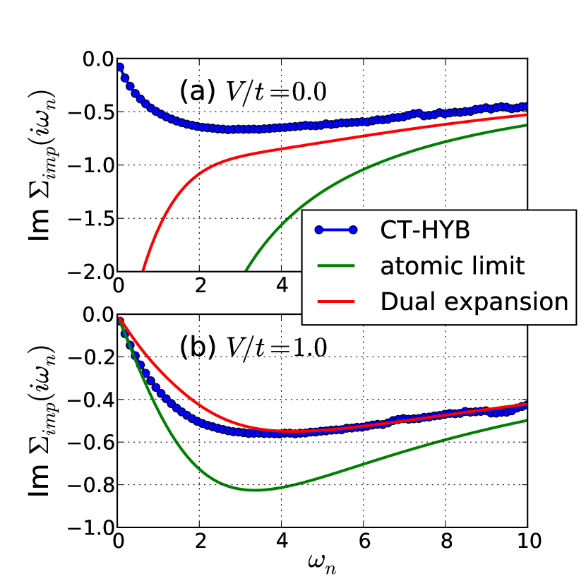
Figure 2: The comparison of the impurity self-energy calculated from the CT-HYB, atomic Hubbard model and the dual expansion method. The parameter sets for the two-orbital Hubbard model are $\beta t=50,U/t=4.0,J/U=0.25,V/t=1.0$. See the text for more details.

II.2 Four-point correlation function $\chi_{12;34}$

The dual expansion, discussed in the above section, requires the knowledge of the atomic four-point correlation function $\chi_{12;34}^{at}$. In the multiorbital case, such a calculation can be hard since the large-dimensional matrix multiplication is time consuming. In this case, one can again use the block diagonal form of the Hamiltonian matrix and employ the look-up routine as we did in the trace calculation. Here, we want to further simplify the calculation by employing the symmetry of $\chi_{12;34}^{at}$. Such a symmetry turns out to be also very useful in the simulation of the impurity four-point correlation function $\chi^{imp}_{12;34}$. Thus, in this section we try to keep our discussion general. We start from the simulation of the $\chi^{imp}_{12;34}$ in the CT-HYB and discuss the symmetries of it afterward. The same symmetry requirements are satisfied by $\chi^{at}_{12;34}$ as well.

Although in the CT-HYB, Wick’s theorem apparently is not supported by the impurity action, the four-point correlation function can be simulated by removing two rows and two columns from the determinant matrix, which results in an expression analogous to those for the CT-INT and the CT-AUX. Effectively, one can still simulate the four-point correlation function as if Wick’s theorem holds. Here, we use the following notation to symbolically represent this expression:

$$\chi_{12;34}:=\langle c_{1}c^{*}_{2}c_{3}c_{4}^{*}\rangle$$ (17)

$$= \overline{\langle c_{1}c_{2}^{*}\rangle\langle c_{3}c_{4}^{*}\rangle}-\overline{\langle c_{1}c_{4}^{*}\rangle\langle c_{3}c_{2}^{*}\rangle}$$

$$= \overline{g_{12}(\omega_{1},\omega_{2})g_{34}(\omega_{3},\omega_{4})}-\overline{g_{14}(\omega_{1},\omega_{4})g_{32}(\omega_{3},\omega_{2})},$$

where labels $12;34$ represent “orbitals, sites, spins,” etc. In the CT-HYB, the two-frequency dependent propagators $g_{\alpha\beta}(\omega,\omega^{\prime})$ is given as

$$g_{\alpha\beta}(\omega_{1},\omega_{2})=-\frac{1}{\beta}\sum_{i,j}e^{i\omega_{1}\tau_{i}}M^{\alpha\beta}_{ij}e^{-i\omega_{2}\tau_{j}}.$$ (18)

It has the following symmetry in Matsubara frequency space:

$$g_{\alpha\beta}(\omega_{1},\omega_{2})=g_{\alpha\beta}^{*}(-\omega_{1},-\omega_{2}),$$ (19)

which reduces the numerical effort by a factor of two. A similar symmetry is also satisfied by $\chi$:

$$\chi_{12;34}=\chi^{\Omega}_{12;34}(\omega,\omega^{\prime})=\chi^{-\Omega,*}_{12;34}(-\omega,-\omega^{\prime}).$$ (20)

In what follows, we denote $\omega=\omega_{1}$, $\omega+\Omega=\omega_{2}$, $\omega^{\prime}+\Omega=\omega_{3}$, $\omega^{\prime}=\omega_{4}$. Equation (20) says, only for $\Omega>0$, $\chi$ needs to be simulated.

Symmetry (20) relates the positive frequencies to the corresponding negative frequencies of $\chi$. It is also possible to find symmetries which connect different $\omega$, $\omega^{\prime}$ in the same $\Omega$ sector. This can be achieved via the fact that $\chi_{12;34}$ is antisymmetric under the exchange $1\Leftrightarrow 3$ and $2\Leftrightarrow 4$:

$$\chi_{34;12}(\omega^{\prime}+\Omega,\omega+\Omega;-\Omega)=\chi_{12;34}(\omega,\omega^{\prime};\Omega).$$ (21)

Combining Eq. (21) with Eq. (20), we have

$$\chi_{34;12}(-\omega^{\prime}-\Omega,-\omega-\Omega;\Omega)=\chi_{12;34}^{*}(\omega,\omega^{\prime};\Omega).$$ (22)

Given the spin configurations of different $\chi$ channels, we find $\chi_{12;34}^{\sigma\sigma;\sigma\sigma}$ satisfies both symmetries in Eqs. (20) and (22). However, $\chi_{12;34}^{\sigma\sigma;\bar{\sigma}\bar{\sigma}}$ only satisfies the symmetry shown in Eq. (20) and the following relation:

$$\chi_{12;34}^{\sigma\sigma;\bar{\sigma}\bar{\sigma}}=\chi_{34;12}^{\bar{\sigma}\bar{\sigma};\sigma\sigma}.$$ (23)

One can implement the symmetries in Eqs. (20) and (22) as follows. (1) $\chi^{\uparrow\uparrow;\uparrow\uparrow}$, $\chi^{\downarrow\downarrow;\downarrow\downarrow}$, and $\chi^{\uparrow\uparrow;\downarrow\downarrow}$ are simulated only for $\Omega>0$. (2) For each specific $\Omega$ considered, Eq. (22) is further applied to $\chi^{\uparrow\uparrow;\uparrow\uparrow}$ and $\chi^{\downarrow\downarrow;\downarrow\downarrow}$. Only for parts of the frequency points in this $\Omega$-sector do $\chi^{\uparrow\uparrow;\uparrow\uparrow}$ and $\chi^{\downarrow\downarrow;\downarrow\downarrow}$ need to be simulated. (3) At the end of the calculation, $\Omega<0$ components are calculated through Eq. (21). (4) $\chi^{\downarrow\downarrow;\uparrow\uparrow}$ is calculated by Eq. (23). In addition to the symmetries shown in Eqs. (20) and (22), it is possible to find more symmetries to relate different frequency sectors.

Before finishing this section, we want to note that the four-point correlation function is useful not only for the physical response function and the dual-expansion scheme, but also relates closely with the extension of the DMFT. In the DF methodRubtsov et al. (2009) and the dynamical vertex approximation (D$\Gamma$A), Toschi et al. (2007) the nonlocal self-energy is constructed from the impurity two-particle vertices.

III Application

As a typical application, we consider here a two-orbital Hubbard model [see the Hamiltonian in Eq. (1)], with rotationally invariant interactions, i.e. $U^{\prime}=U-2J,U^{\prime\prime}=U^{\prime}-J$. To make a link with realistic material systems, this multiorbital Hubbard model can be viewed as an effective model for the $e_{g}$-orbital systems. The rotational invariance of the interaction term is not obligatory in the CT-HYB solver; here, we use it only as one possible situation. By making use of the DMFT, the two-orbital Hubbard model has been studied by many groups. Lu et al. (2008); Werner and Millis (2007); Sentef et al. (2009); Peters et al. (2011); Inaba and Koga (2007); Werner and Millis (2006); Koyama et al. (2009); de’ Medici (2011); de’ Medici et al. (2011) These calculations are either based on a semicircular density of states, which corresponds to the Bethe lattice, or they employ an impurity solver with certain limitations in temperature or interaction strength. Here, we solve the DMFT equation at finite dimension and temperatures. In these cases, the DMFT loop cannot be closed by a simple relation in the imaginary-time space like on the Bethe lattice. Thus, our dual-expansion method discussed in Sec. II.1 turns to be a decisive tool. Our calculations are mainly performed on ordinary desktop computers.

Compared to the single-orbital case, two issues in a multiorbital model are of obvious interests:
(1) What is the effect of the orbital fluctuations? The general believe is, that it is competitive to the Coulomb interaction. As a result, the metallic state can be stabilized up to a large interaction valueInaba et al. (2005); Koga et al. (2002).
(2) How does the Hund’s coupling modify the transition from the metal to Mott insulator (MIT)? It is known that the two-orbital Hubbard model behaves quite differently with and without $J$. Lu et al. (2008); Werner and Millis (2007)
The phase diagrams of the two-orbital Hubbard model can be found in Refs. Werner and Millis, 2007 and de’ Medici, 2011. Here we study, in particular, the coexistence region for different values of $J$ in Fig. 3 (a), which indicates the MIT is of first order. Compared to the phase diagrams for the Bethe lattice, Werner and Millis (2007); de’ Medici (2011) the reduction of the spatial dimension does not change significantly the critical Coulomb interaction value of $U_{c}$ when it is normalized by the full bandwidth. However, $U_{c}$ becomes larger compared to the single-orbital model, which confirms that the orbital fluctuation stabilize the metallic phase. With the increase of the Hund’s rule coupling $J$, we found the coexistence region to become smaller. For the two values of $J/U$ in our calculations, the reduction is about 0.2 eV. On the other hand, Bulla et al. Pruschke and Bulla (2005) found, for $J/U>0.25$, the transition to be of second order. At $J/U=0.25$, our results show that the coexistence region still has a reasonably large width. Thus, we believe that even for $J/U>0.25$, the MIT remains first order. Whether, the coexistence region completely disappears with the further increase of $J/U$ deserves more investigations.

On the right-hand side of Fig. 3, two different solutions of the local density of state, that is, $A(\omega)$, are displayed for $U/t=8.4$. They correspond to the metallic, see Fig. 3 (b), and insulating states [see Fig. 3 (c)] in the coexistence region. $A(\omega)$ is obtained by using the stochastic analytical continuation directly on the Matsubara data of $G_{imp}(i\omega_{n})$. Beach (2004)

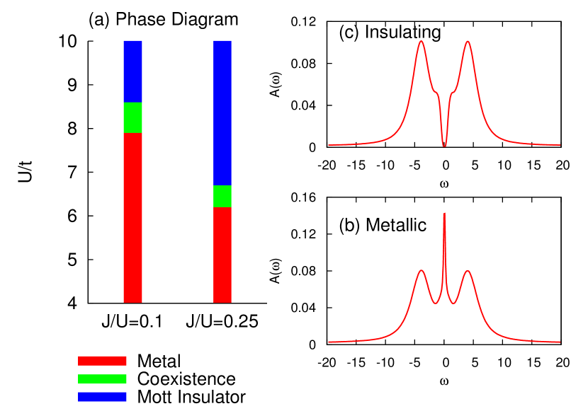
Figure 3: The phase diagram of the two-orbital Hubbard model at half filling. The MIT at $\beta t=50$ for two values of $J/U$ are shown as histograms. The two local density of states on the right-hand side correspond to the two solutions for $U/t=8.4,J/U=0.1$.

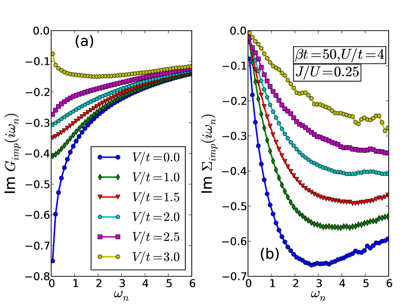
Figure 4: Behavior of the impurity self-energy and Green’s function around the metal-to-band-insulator transition as functions of the hybridization strength $V/t$.

In Fig. 4, the typical behavior of the metal-to-band-insulator transition is shown by calculating the impurity Green’s function and the corresponding self-energy as a function of the hybridization. Increasing the hybridization $V/t$ tends to open a band gap. Furthermore, with the increase of $V/t$, the impurity Green’s function at the lowest Matsubara frequency becomes smaller and finally approaches zero [see Fig. 4 (a)]. The metal-to-band-insulator transition happens somewhere between $V/t=2.5$ and $3.0$ for $U/t=4$. This transition is not visible from the self-energy plot, where $\Sigma_{imp}(i\omega_{n})$ behaves similarly for different values of $V/t$. The slope, that is, $\partial\Sigma_{imp}(\omega)/\partial\omega|_{\omega_{0}}$, remains negative for all hybridization strengths [see Fig. 4 (b)]. In contrast, the slope of the local Green’s function around $\omega_{0}$ has different signs before and after the metal-insulator (band) transition.

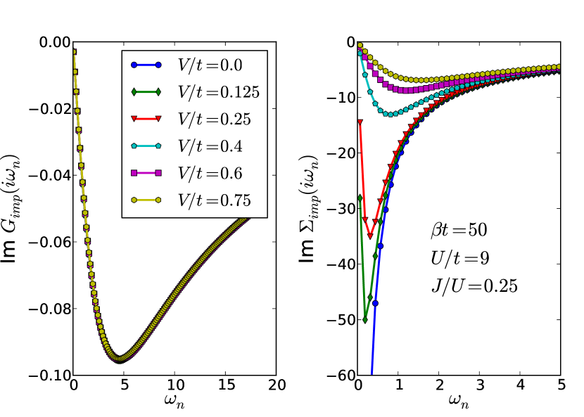
Figure 5: Similar to Fig. 4, but with different interaction strength $U/t=9$, where a Mott-insulating state is found at $\Delta/t=0,0.125,0.25$. The increase of the hybridization between two orbitals greatly changes the behavior of the self-energy, while it leaves the one-particle Green’s function essentially unchanged.

Increasing further the value of $U/t$ strengthens both the intra- and interorbital interactions. Finally, for values of $U/t$ of the order of the noninteracting bandwidth, the metal to band-insulator transition is replaced by the Mott-insulator-to-band-insulator crossover as a function of the hybridization strength $\Delta/t$. This behavior is displayed in Fig. 5. In contrast to the metal to band-insulator transition shown in Fig. 4, in Fig. 5 (with a choice of $U/t=9$), the local Green’s function stays nearly unchanged under modifying the hybridization strength $V/t$, that is, $G_{imp}$ shows an insulating behavior for all values of $V/t$. However, for different values of $V/t$, the insulating nature is indeed different. This can be seen from the variation of the self-energy function shown in the right-hand side of Fig. 5. Increasing $V/t$, results in increasing of $\partial\Sigma(\omega)/\partial\omega|_{\omega_{0}}$ for any finite $V/t$, indicating the crossover from Mott-insulator to band-insulator behavior. Fuhrmann et al. (2006)

By applying the symmetries presented in Sec. II.2, we show the results for the interorbital and intraorbital reducible spin susceptibilities in Fig. 6 for $\beta t=20,U/t=6,J/U=0.25$, and $V/t=0$, with $a,b$ the orbital indices:

$$\tilde{\chi}^{spin,ab}_{\Omega}(\omega_{n},\omega^{\prime}_{n})=\frac{1}{2}(\tilde{\chi}_{ab,\Omega}^{\sigma\sigma,\sigma\sigma}-\tilde{\chi}_{ab,\Omega}^{\sigma\sigma,\bar{\sigma}\bar{\sigma}})$$ (24)

$\tilde{\chi}^{spin,ab}_{\Omega}(\omega_{n},\omega^{\prime}_{n})$ are the impurity susceptibilities with the subtraction of the impurity bubble susceptibilities. They are plotted as functions of the two fermionic frequencies $\omega_{n},\omega_{n}^{\prime}$ for fixed $\Omega=0$. While here only the $\Omega=0$ component is given, the implementation discussed in Sec. II.2 works for any value of $\Omega$. Figures 6(a) and 6(b) refer to the three-dimensional (3D) plots of $\tilde{\chi}^{spin,ab}_{\Omega}(\omega_{n},\omega^{\prime}_{n})$; the corresponding 2D top-view plots are shown in Figs. 6(c) and 6(d). Based on the CT-HYB, the four-point correlation functions were recently also calculated for the effective one and four-orbital systemsBoehnke et al. (2011); Park et al. (2011) for different problems. Another efficient and stable, but approximate, algorithm can be found in Ref. Kuneš, 2011.

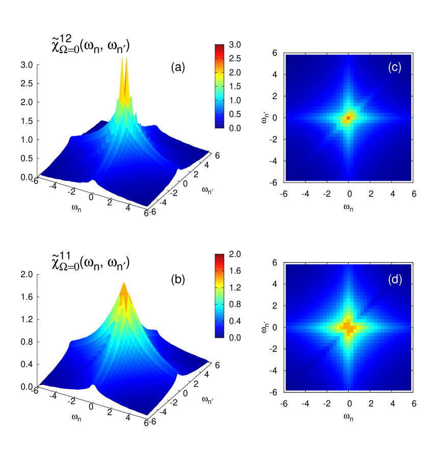
Figure 6: The interorbital, that is, $\tilde{\chi}_{\Omega=0}^{12}$, and intraorbital, that is, $\tilde{\chi}_{\Omega=0}^{11}$, components of the reducible impurity two-particle susceptibility for $\beta t=20,U/t=6,J/U=0.25$.

From Fig. 6, we see that the reducible two-particle susceptibility $\tilde{\chi}_{\Omega=0}^{spin,ab}(\omega_{n},\omega_{n^{\prime}})$ decays rather fast as a function of $\omega_{n}$ and $\omega_{n^{\prime}}$. The dominant contribution comes from the elements with $\omega_{n}=0$, or $\omega_{n^{\prime}}=0$, or $\omega_{n}=\omega_{n^{\prime}}$. For our parameter set, the interorbital spin susceptibility shows a sharper structure than the intraorbital one, which can be viewed as a precursor of the possible orbital antiferromagnetic order.

IV Conclusion

In this paper, we showed how the high-frequency tail of the self-energy can be calculated in a controlled manner from the dual transformation in CT-HYB. This scheme provides an efficient recipe for finite-dimension DMFT studies when taking the CT-HYB as an impurity solver. Our procedure is based on a Matsubara frequency space simulation and produces more moments from the dual expansion. Thus, it generates an improved high-frequency self-energy behavior. Most importantly, it does not introduce any additional numerical cost to the runtime simulation. We also simulated the four-point correlation function for different spin configurations in the particle-hole channel. To this end, we implemented different symmetries to reduce the memory and CPU requirements without losing accuracy.

As a first application, we demonstrated the usefulness of our method for a two-orbital model with a general on-site interaction. From this study, we deduced a substantial influence of the Hund’s rule coupling on the metal-insulator transition phase diagram, especially on the coexistence region. In particular, we find that for any finite value of $J/t$, the MIT stays first order.

Our scheme is also of particular use for connecting the DF method, which many be viewed as a nonlocal extension of the DMFT, with a priori DFT techniques. A multiorbital DF calculation will be especially interesting and rewarding for the DFT + DF study of material systems. In such study, the CT-HYB effectively works on an impurity problem with the DFT dispersions as input. Thus, one has a good control on the ”minus-sign” problem. The high-momentum resolution, provided by the DF algorithm, makes the result ready to be compared with experiments, such as ARPES data.