Quantization based Recursive Importance Sampling
Abstract
We investigate in this paper an alternative method to simulation based recursive importance sampling procedure to estimate the optimal change of measure for Monte Carlo simulations. We propose an algorithm which combines (vector and functional) optimal quantization with Newton-Raphson zero search procedure. Our approach can be seen as a robust and automatic deterministic counterpart of recursive importance sampling by means of stochastic approximation algorithm which, in practice, may require tuning and a good knowledge of the payoff function in practice. Moreover, unlike recursive importance sampling procedures, the proposed methodology does not rely on simulations so it is quite generic and can come along on the top of Monte Carlo simulations.
We first emphasize on the consistency of quantization for designing an importance sampling algorithm for both multi-dimensional distributions and diffusion processes. We show that the induced error on the optimal change of measure is controlled by the mean quantization error.
We illustrate the effectiveness of our algorithm by pricing several options in a multi-dimensional and infinite dimensional framework.
Keywords: monte carlo simulation, importance sampling, stochastic approximation, vector quantization, functional quantification.
Introduction
In this paper, we are interested in one of the most basic problem of numerical probability which consists in the computation of the expectation
| (1) |
where is a random vector taking values in a Banach space and is a Borel function such that . When the space is (equipped with the Euclidean norm) we will refer to the finite (multi) dimensional setting and when the space is (equipped with the supremum norm) to deal with the case where is a continuous path-dependent diffusion process, we will refer to the infinite dimensional setting. For instance in mathematical finance, computing the price of an option and the sensitivities of this price with respect to some parameters amounts to estimate such a quantity. When no closed or semi-closed formulas are available, one often relies on Monte Carlo simulation which remains the most widely used numerical method in this context.
Variance reduction methods are often used to increase the accuracy of a Monte Carlo simulation or reduce its computation time. The most common variance reduction methods are antithetic variables, conditioning, control variate, importance sampling and stratified sampling. Adaptive variance reduction methods have been recently investigated to take advantage of the random samples used to compute the expectation above in order to optimize at the same time the variance reduction tool (see [11] and the references therein). In practice, it is not clear that this adaptive one step Monte Carlo procedure is better than the basic two step procedure: optimizing the variance reduction tool (e.g. the optimal change of measure in an importance sampling framework) using a small number of samples, then computing the expectation of interest with this optimized parameter.
In this paper, we are interested in variance reduction by importance sampling (IS). We denote by the probability density function of and we consider a parameterized family of density functions : we will choose in the finite dimensional setting and , where is the dimension of the Brownian motion driving the dynamic of the -dimensional process , when dealing with the infinite dimensional setting. This general framework is the one investigated in [15]. In this introduction we will present the importance sampling paradigm in the finite multi-dimensional case, we set . We suppose that , , where denotes the Lebesgue measure on and we set . Moreover, we focus throughout all the paper on importance sampling by mean translation, we will consider that for all , for all , . The basic idea of IS is to introduce the parameter in the above expectation (1) using the invariance by translation of the Lebesgue measure, for every
| (2) |
and among all these random variables with the same expectation, we want to select the one with the lowest variance, the one with the lowest quadratic norm
A reverse change of variable shows that:
| (3) |
Now if the density function of satisfies
| (4) |
and
| (5) |
then, one shows that the function is finite, convex and goes to infinity at infinity, thus , where is the gradient of , is non empty (for a proof, we refer to [15]).
Now, if admits a representation as an expectation, then it is possible to devise a recursive Robbins-Monro (RM) procedure to approximate the optimal parameter minimizing , namely
| (6) |
where is an sequence of random vectors having the distribution of , is a positive deterministic sequence satisfying,
and is naturally defined by the formal differentiation of : for every ,
| (7) |
IS by means of stochastic approximation has been investigated by several authors (see e.g. [8], [5] and [6]) in order to estimate the optimal change of measure by a RM procedure. It has recently been studied in the Gaussian framework in [1] (see also [2]) where (7) is used to design a stochastic gradient algorithm. However, the regular RM procedure (7) suffers from an instability issue coming from the fact that the classical sub-linear growth Assumption in quadratic mean in the Robbins-Monro Theorem
| (8) |
is only fulfilled when is constant, due to the behaviour of the annoying term as goes to infinity. Consequently, can escape at infinity at almost every implementation as pointed out in [1]. To circumvent this problem, a “projected version” of the procedure based on repeated reinitializations when the algorithms exits from an increasing sequence of compact sets (while the step keeps going to 0) was used. This approach is known as the projection “ la Chen” (see for instance [3], [4] and [14]). A central limit theorem for this version of the recursive importance sampling algorithm is proved in [13]. This kind of technique forces the stability of the algorithm and prevents explosion. From a numerical point of view, this projected algorithm is known to converge if the sequence of compact sets have been specified suitably, which is not an easy task in practice.
In [15], the authors propose a third change of variable to plug back the parameter into
| (9) |
which has a known controlled growth rate at infinity in common applications. For instance, if we suppose that there exists , such that
we can define a new function by setting
| (10) |
Under additional assumptions on the density function , they derive a new stochastic approximation algorithm using which satisfies the sub-linear growth condition (8) so that it converges and is stable without having to apply projection technique. They also extend this construction to exponential change of measure (Esscher transform) and to diffusion process using Girsanov transform. However, from a numerical point of view, the tuning of the algorithm needs a good knowledge of the behavior of at infinity. In practical implementations, recursive importance sampling methods using stochastic implies specific tuning of the step sequence or the sequence of compact sets which in both cases strongly depends of the payoff function .
In order to get rid of this problem, [12] proposes an optimization Newton’s algorithm to estimate the optimal change of measure in a Gaussian framework. They approximate and (based on the representation (7) with , ) using Monte Carlo simulation with samples
where is an sequence of -dimensional standard normal vectors. The (unique) minimum of is approximated by the (unique) zero of which can be computed using a deterministic Newton-Raphson algorithm. Moreover, several asymptotic properties are addressed.
Deterministic optimization using a large deviation argument has been investigated in [7]. The optimal change of measure is selected as a local maximum of . This can be achieved only under some regularity assumptions on the function . Moreover, from a theoretical point of view this choice is not optimal.
In this work, we propose and study an alternative deterministic procedure which is not adaptive and does not need specific payoff-dependent tuning. The optimal change of measure is estimated using a robust and automatic Newton-Raphson’s algorithm combined with optimal (vector and functional) quantization. The main advantage of our procedure is that it can be used as a generic variance reduction method which comes upstream the Monte Carlo simulation framework. Moreover, we will focus on one very common situation in mathematical finance, that is, Monte Carlo simulation that are based on multi-factor Brownian diffusions. Indeed, the presented method easily extends to this framework using quadratic optimal functional quantization of stochastic processes (see [19]). It is particularly adapted for financial institutions since the methodology we propose can come along on the top of Monte Carlo simulations. Numerical tests ilustrate the effectiveness of our approach in both multi-dimensional and infinite dimensional frameworks.
The paper is organized as follows. Section 1 presents several results about vector and functional quantization that are required in the following. We focus on the functional quantization of diffusion processes. Section 2 presents the quantization based recursive importance sampling algorithm. The emphasis is on the consistency of quantization for designing an importance sampling algorithm for both multi-dimensional distributions and diffusion processes. We show in particular that the induced error on the optimal change of measure is controlled by the mean quantization error. In section 3, we provide numerical experiments of our approach by considering option pricing problems arising in mathematical finance.
1 Some results on optimal quantization
Before, dealing with the construction of the quantization based IS algorithm, we provide with some background on quantization of Hilbert spaces and Gaussian processes viewed as -valued random vectors.
1.1 Introduction to quantization of random variables
Let . The principle of the -quantization of a random variable taking its values in a separable Hilbert space is to study the best -approximation of by -valued random vectors taking at most values. The norm is the usual norm on defined by . When , we talk about quadratic optimal quantization. If , one speaks about vector quantization. When is an infinite dimensional Hilbert space like endowed with the usual norm , we talk about functional quantization.
Definition 1.1 (Voronoi tessellation).
Let and be a -tuple referred to us by a quantizer and let Proj be a projection following the closest neighbour rule. Then, the Borel partition of defined by Proj, and satisfying
is called a Voronoi tessellation of induced by .
One defines the Voronoi quantization of induced by by
The discrete random variable (one will sometimes simply write if there is no ambiguity) is the best -approximation of among all measurable random variable taking values in . In fact, for any random variable , we have
so that .
For any fixed -quantizer , we associate the -mean error induced by . One aims at finding a tuple which minimizes the -mean error over . It amounts to minimizing the function
The function reaches its minimum at one (at least) tuple called an optimal -quantizer. This infimum is in general not unique, except in some cases, in particular when and the density of is log-concave. Note that card() if card(supp()). Moreover, the -mean quantization error converges toward and for non-singular -valued random vectors, the rate of convergence of convergence of is ruled by the so-called Zador Theorem (see [10]).
Theorem 1.1.
Assume that for some . Let denote the density of the absolutely continuous part of (possibly, ). Then,
| (11) |
where is a strictly positive depending only on and on the dimension .
For further theoretical results on optimal vector quantization we refer to [10]. One of the important issues for the Numerical Probabilities viewpoint is to compute the optimal quantizers and the associated weights (for the applications to Numerical Probabilities in the finite dimensional case, see the seminal paper [18]). However, due to the non-uniqueness of the optimal quantizers in the general framework, specially when with , we are usually leaded to search for stationary quantizers, -quantizers satisfying . We will see further on that stationary quantizers are an important class of quantizers for numerics. The commonly used result is the quadratic case (when ) recalled below.
Definition 1.2 (Stationarity).
Let be an -quantizer and its associated Voronoi partition. The random vector is called a stationary -quantization of if it satisfies
| (12) |
(-negligible boundary of the Voronoi cells) and
We have in particular, .
1.2 Some backgrounds on functional quantization
A rigorous extension of optimal vector quantization to functional quantization is done in [16]. The vector quantization problem is transposed to random vectors in an infinite dimensional Hilbert space, in particular, to stochastic processes viewed as random vectors with values in . In [20], numerical performances of quadratic functional quantization with applications to finance is investigated. In particular, the roles played by product quantizers and the so-called Karhunen-Loève (K-L) expansion of Gaussian processes are pointed out.
In what follows, we will start by the functional quantization of the standard Brownian motion since everything can be made explicit for this process. Then we will show how to construct from optimal quadratic functional quantization of Brownian motion explicit (non-Voronoi) quantization of Brownian diffusions.
Assume that the separable Hilbert space is , with . One defines the covariance operator of the Brownian motion , for every by
This operator is symmetric positive and can be diagonalized in the K-L orthonormal basis of with eigenvalues given by
Moreover, one may expand the paths of on this basis,
| (13) |
Using Fubini’s Theorem and the orthonormality of the K-L basis, one obtains for ,
where denotes the Kronecker symbol. Consequently, the Gaussian sequence is pairwise non-correlated so that these random variables are independent. Hence, (13) can be written
where , , is an i.i.d. sequence of random variables with standard normal distribution.
Now the idea of product functional quantization using at most elementary quantizers is to quantize these random coordinates , for every , one considers an optimal -quantization () of , denoted where , is the unique optimal -quantizer of the normal distribution and , . For large enough, we set , (which is the optimal 1-quantization) and we define the product quantizer by (the finite sum)
The product quantizer that produces the above Voronoi quantization is defined by
and for every multi-index , the associated Voronoi cell of is
Moreover, from the independence of the normal random variables the weights can be computed explicitly
For numerical purposes, one may be interested by the theoretical rate of convergence for the quantization error of the Brownian motion and the stationarity of K-L product quantizer.
Proposition 1.2 (stationarity, see [20]).
The product quantizer of the Brownian motion defined above is a stationary quantizer,
Proposition 1.3 (convergence rate, see [16]).
For every , there exists an optimal product quantizer of size at most , denoted of the Brownian motion defined as the solution to the minimization problem
| (14) |
Furthermore, these optimal product quantizer induces a rate optimal sequence,
for some real constant
To conclude this section, we shortly describe a constructive way to quantize scalar brownian diffusions (for more details see [20]). The rate is like for the Brownian motion as soon as the diffusion coefficient is not too degenerate. Consider the homogeneous Brownian diffusion process:
where and are continuous on with at most linear growth ( ) so that a weak solution to the equation exists. Let be a sequence of rate-optimal K-L product quantizers of the Brownian motion. For every multi-index , with , consider the solution of the following integral equations
| (15) |
where is the first derivative of . To simplify notations we consider the simpler notation for the multi-index . Now set
| (16) |
The process is a non-Voronoi quantization but it is easily computable once the above integral equations are solved since the weights are known. However the ODE (15) has no explicit solution in general. Then, for numerical implementation purposes, we use discretization schemes like Runge-Kutta one to estimate these quantizers. One shows that the quantized process converges toward the process with respect to the quadratic norm and the rate of convergence is given by the following result.
Proposition 1.4 (See [17]).
Assume that is differentiable, is positive twice differentiable and that is bounded. Then
1.3 Quadrature formulae for numerical integration
We conclude this first section on optimal (quadratic) quantization by illustrating how to use it for numerical integration of functions defined on the Hilbert space . We provide some quadrature formulae using the above quantization errors. We refer to [20] for the proofs. The main idea is that we know that is close to in distribution and if one has a numerical access to the -quantizer with the associated weights sequence of the quantization then for every Borel functional , the computation of the expectation
is straightforward. The proposition below gives some error bounds for based on -quantization error ( or 4) of .
Let be a stationary quantizer for with its associated Voronoi quantization and be a Borel functional defined on .
-
(i)
Inequality for convex functionals: If is convex then
-
(ii)
Lipschitz functionals:
-
–
If is Lipschitz continuous then
-
–
Let be a nonnegative convex function such that . If is locally Lipschitz with at most -growth, then and
-
–
-
(iii)
Differentiable functionals: If is differentiable on with an -Hölder differential D (), then
Other quadrature formulae can be derived based on regularity assumptions on (for more details we refer to [20]).
2 Quantized importance sampling algorithm
2.1 The finite-dimensional setting
In order to derive the existence of a unique minimum for the function , we make the following assumption:
Assumption 1.
Moreover, the differentiation of the quadratic norm (with respect to ) defined by (3) is required further on and we need for this purpose the following assumptions on the probability density function :
Assumption 2.
The density function is twice differentiable and satisfies for some
-
(i)
as .
-
(ii)
such that , , where is the Hessian of .
Proposition 2.1.
Suppose that Assumptions 1 and 2 are satisfied and the function satisfies
Then, the function defined by (3) is finite, strictly convex, differentiable on , goes to infinity as goes to infinity. As a consequence, the function admits a unique global minimum satisfying
and the gradient is given by
| (17) |
Moreover, if satisfies
| (18) |
and,
| (19) |
then, is twice differentiable and its hessian is given by
| (20) |
Proof..
For every , is strictly concave so that is strictly convex, hence the function is strictly convex. Combining Fatou’s lemma and Assumption 1, one easily obtains that .
In order to get the formal differentiation representation (17) we have to check the domination property for , for every . The log-concavity of implies that for every and ,
Hence using Assumption 2 (i) yields
| (21) |
so that
To justify the formal differentiation of to get (20) we proceed as follows. Let . Using Assumption 2 yields for every
and,
Consequently, , we have
where and . Using the assumption (18) implies that . Moreover, using another change of variable and (21) yields
so that (19) implies for every
Consequently, the family is -uniformly integrable. This provides the expected representation (20). ∎
Examples of distributions
-
The Normal distribution
-
The logistic distribution
Assumption 1 is satisfied. Assumption 2 holds with .
-
The hyper-exponential distributions
where is a positive polynomial function.
The main idea is that we know that , and can be approximated by
| (22) | ||||
| (23) | ||||
| (24) |
using an -quantizer with the associated weights sequence of the quantization . The computations of (22), (23) and (24) are straightforward. For large enough, for some , so that is also strictly convex and goes to infinity as goes to infinity. Moreover, it is clear that is differentiable. Hence, there exists a unique such that . Moreover, for large enough, the Hessian matrix is symmetric positive definite for every .
The following proposition describes the asymptotic behavior of as . It shows, as expected, that as . First we need the following assumption:
Assumption 3.
The function is positive, convex on and satisfies
-
(i)
F is Lipschitz on ,
-
(ii)
, such that and for all , .
Proposition 2.2 (Convergence of ).
Consider an -optimal stationary quantizer of size with its associated quantization . Assume that the assumptions of Proposition 2.1 and that Assumption 3 are satisfied. Then, we have
where is the unique global minimum of defined by (22).
Proof.
The first step of the proof consists in showing that the function converges locally uniformly to the continuous function . Let and . We have
Using the log-concavity of , Assumption 2 and the inequality yields, for every
Consequently, we have
hence, Schwarz’s and Hölder’s inequalities implies for every
Now is convex since F is and is increasing and convex on . Consequently, by Jensen’s inequality
Using similar arguments, we have: , , . Finally, we obtain for some positive constant independent of and
So that converges locally uniformly to .
Now let . being continuous at and strictly convex
The local uniform convergence of to ensures that
Assume that satisfies . The convexity of implies that
so that,
Since is the unique global minimum of , we have . Consequently, for and converges to . Combining the local uniform convergence of to and the continuity of at , we obtain that , as . This concludes the proof. ∎
A classical method for estimating , for solving the system of nonlinear equations is Newton-Raphson’s algorithm:
| (25) |
Newton-Raphson’s algorithm is attractive because it converges rapidly from any sufficiently good initial guess under standard assumptions. Indeed, since is the unique solution of , is continuously differentiable on and is a symmetric positive-definite matrix for all , then the sequence defined by (25) is known to converge toward if is sufficiently close to .
At this stage, it is natural to characterize the rate of convergence of to . To this end, first we need to obtain some error bounds for , , for some .
Assumption 4.
The function is -Hölder.
Proposition 2.3.
Assume that Assumptions 1, 2, 3 and 4 hold. Let be an -optimal stationary quantizer of size and the associated Voronoi quantization. Then, for every , for every
Hence, converges locally uniformly to .
Proof..
Let , and . We have
First we take care of the first term of the above sum. Using Assumption 2 (i), Assumption 3 (i) and (21), yield
Now, we focus on the second term. Using similar arguments than the ones used in the proof of Proposition 2.2 and Assumption 2 (i) yield
Finally, using (21) and Assumption 4 for the last term implies
Using similar arguments than the ones used in the proof of Proposition 2.2 yields
∎
Now we are in position to characterize the convergence rate of toward . The following result shows that as expected the error is controlled by the quantization error.
Theorem 2.4.
Assume that Assumptions 1, 2, 3 and 4 hold. For every , there exists such that, if , then the sequence defined by (25) converges to . Moreover, the convergence rate of to is based on -quantization error in the sense that
Proof..
We define the norm , for . Since is non-singular,
where . Choose sufficiently small that . We can choose sufficiently small such that if then
| (26) | |||
| (27) | |||
| (28) |
The continuity of at , the non-singularity of and the continuous differentiability of at ensures the existence of such an . The existence of an such that the sequence converges to if follows using the same arguments applied to .
The convergence of to ensures the existence of such that if , . Hence (26), (27) and (28) hold for , .
Now, the recursive algorithm (25) can be written
| (29) |
with , and .
Using the following equality
and taking norms in (29) yields
| (30) |
Let and such that so that converges toward . The continuity of , , and at and the non singularity of and yield
Moreover, for , using (27) we have
Finally, Proposition 2.3 and the choice of yield
so that as . ∎
Remark 2.1.
When is a -dimensional gaussian vector, Assumptions 2 and 4 are satisfied with so that if is an -optimal quantizer with its associated Voronoi quantization , Theorem 1.1. implies the following error bound in Theorem 2.4
In practice, only a rough estimate of the optimal change of measure parameter is needed. According to our numerical results, optimal quantization grids of size (depending on the dimension ) are enough. Concerning , it can be computed with a high precision by a few steps (usually less than 10) of the Newton-Raphson’s optimization procedure (25).
For the sake of simplicity we used the classical Lipschitz continuous assumption on but other error bounds can be derived by replacing Assumption 3 by other smoothness assumption.
2.2 Quantized importance sampling for Brownian diffusions
In this section, we extend the Newton-Raphson’s algorithm to the infinite dimensional setting, the case of path-dependent diffusion. We will rely on the Girsanov transform to play the role of mean translator. To be more precise, we consider a -dimensional Itô process solution to the stochastic differential equation (S.D.E.)
| () |
being a dimensional standard Brownian motion and where is the stopped process at time t, , are measurable with respect to the canonical predictable -field on .
Under the following assumption
| () |
strong existence and uniqueness of solutions for can be proved (for more details, see [21]). We aim at devising a robust and automatic Newton-Raphson’s algorithm based on functional quantization inspired from Section 2.1 for the computation of
where is a Borel functional defined on such that
| (31) |
In this functional framework, the invariance by translation of the Lebesgue measure (2) is replaced by Girsanov Theorem. We consider a translation process given by which is slightly less general than the ones used in [15]. Indeed, they considered translation processes of the form defined for every and by
is a prespecified bounded Borel function. In what follows, we can easily adapt to this kind of translation processes but for the sake of simplicity, we prefered to focus on this simple case.
It follows from Girsanov Theorem that for every
where denotes the solution to . Among all these estimators we want to select the one with the lowest quadratic norm so that we want to solve the following minimization problem
Another Girsanov Theorem yields
| (32) |
In view of numerical implementation of a Newton-Raphson’s algorithm to estimate a minimum of , we are lead to consider a (non trivial) finite dimensional subspace of spanned by an orthonormal basis . Like for the finite dimensional framework, our procedure will be based on the representation (as an expectation) of the first differential and the second differential of on combined with functional quantization of .
Proposition 2.5.
Assume that for some as well as assumptions and (31) hold. Then the function defined by (32) is finite, strictly convex on and
Moreover, the function is twice differentiable at every and for every ,
| (33) | ||||
| (34) |
where is twice differentiable with
Proof..
Owing to Hölder’s inequality of conjugate exponents , we have for every
since the Doléans exponential is a true martingale for any . The function is strictly convex since the function is and exp is strictly increasing and strictly convex.
Now, using the trivial equality
and the reverse Hölder’s inequality with conjugate exponents yields
by the martingale property of the Doléans exponential. Let such that . We have , so that goes to infinity as goes to infinity.
The random functional from into (for all ) is twice differentiable since
and,
where is a bounded linear operator from into . Using the Cauchy-Schwarz and the Burkholder-Davis-Gundy inequalities, its operator norm satisfies . Consequently, by the composition rule, we derive that is twice diffentiable from into for any . Moreover, for every , we have , and .
The target of the stochastic algorithm investigated in [15] is the minimum of the restriction of Q on , which satisfies . Like for the static framework, in order to approximate and (which can be seen respectively as the -tuple and as an symetric positive definite matrix ) for every , we consider an (non-Voronoi) -functional quantization of given by (16). Hence, for every , we approximate , and by respectively , and defined by
where , and , , .
Hence, we compute the minimum of by devising the following Newton-Raphson algorithm
| (35) |
where for every , and , , .
Remark 2.2.
Like for the static framework (see Proposition 2.2 and Theorem 2.4), the convergence of toward and its convergence rate can be established under assumptions similar to the finite dimensional framework.
3 Numerical illustrations
In the following of this section, we illustrate the performance of these generic variance reduction algorithms both in the finite dimensional framework and in the diffusion framework. The numerical simulations are done in Scilab 5.3.
3.1 Finite dimensional setting
Basket options: We consider basket options with payoffs given by where is the vector of weights, denotes the strike, is the maturity and is the price at maturity of the ith asset. We assume that each of the assets under the risk-neutral measure has a price given by a Black-Scholes model driven by the vector of independent Brownian motions ,
where is a Gaussian vector of size . We price this basket option with different values of the number of assets and the strike . The quantization grids have the same size and the number of Monte-Carlo simulations is 100,000 in every case. Note that for each value of and each value of the strike , the prices are computed using the same pseudo-random number generator initialized with the same seed.
The numerical results are reported in Table 1. In this table, the first two columns correspond to the different values of the dimension and the strike . The third and fourth columns correspond to the crude Monte-Carlo estimator and its associated variance. The fifth and sixth columns refer to the Monte-Carlo estimator and its variance using the optimal change of measure computed with our Newton-Raphson’s algorithm.
| d | K | Price MC | Variance MC | Price QIS | Variance QIS |
|---|---|---|---|---|---|
| 2 | 50 | 5.475 | 62.26 | 5.490 | 7.86 |
| 55 | 3.294 | 40.54 | 3.309 | 4.33 | |
| 60 | 1.873 | 24.03 | 1.885 | 2.03 | |
| 3 | 50 | 4.751 | 42.01 | 4.760 | 5.88 |
| 55 | 2.523 | 24.26 | 2.545 | 2.82 | |
| 60 | 1.237 | 12.38 | 1.221 | 1.01 | |
| 4 | 50 | 4.333 | 32.03 | 4.343 | 4.64 |
| 55 | 2.086 | 16.93 | 2.089 | 2.01 | |
| 60 | 0.882 | 7.29 | 0.868 | 0.58 | |
| 5 | 50 | 4.061 | 26.05 | 4.057 | 3.99 |
| 55 | 1.781 | 12.77 | 1.777 | 1.51 | |
| 60 | 0.642 | 4.63 | 0.647 | 0.35 | |
| 6 | 50 | 3.843 | 22.10 | 3.830 | 3.50 |
| 55 | 1.566 | 10.02 | 1.553 | 1.19 | |
| 60 | 0.506 | 3.25 | 0.494 | 0.22 |
We can see in this example that our Quantization based Importance Sampling algorithm does reduce the variance by a factor varying from 6 up to 15. Note that it does not require any Monte-Carlo simulations to compute the optimal change of measure and unlike most adaptive importance sampling algorithm it does not need specific parameter tuning. One does not have to set up complicated adjustments when using it, it is fully generic and automatic. Hence, it is a very interesting variance reduction procedure to be used in an industrial way.
Spark spread option: We consider now an exchange option between gas and electricity (called spark spread) with payoff given by where and denote electricity and gas spot prices at maturity , is a heat rate and is the generation cost. This kind of payoff appears in the pricing of power plant. We assume that the dynamic of electricity and gas spot prices follows the SDE:
where and are two independent Brownian motions. The stochastic processes , are Ornstein-Uhlenbeck processes:
Writing spot prices as exponential of a sum of Ornstein-Uhlenbeck processes is a very common way to reproduce the mean reversion behavior of commodity spot prices. This model was first proposed by Schwartz in [22]. In this example, the dimension is equal to 2. The quantization grids have the same size and the number of Monte-Carlo simulations is 100,000 in every case.
The numerical results are summarized in Table 2 where we price the spark spread option for different values of . We see that our Quantization based IS algorithm perfoms well again. In any case, the variance is divided by at least 13. Once again the Newton-Raphson algorithm proposed converges quickly, five iterations are enough to get a very accurate estimate of .
| C | Price MC | Variance MC | Price QIS | Variance QIS |
|---|---|---|---|---|
| 0 | 7.933 | 221.01 | 7.957 | 16.48 |
| 3 | 6.681 | 189.24 | 6.757 | 13.32 |
| 5 | 6.024 | 176.93 | 6.049 | 11.54 |
| 8 | 5.081 | 153.44 | 5.083 | 9.16 |
| 10 | 4.575 | 141.09 | 4.531 | 7.81 |
| 12 | 4.057 | 125.49 | 4.032 | 6.61 |
3.2 Infinite dimensional setting
We consider three different basis of
-
•
a polynomial basis composed of the shifted Legendre polynomials defined by
(ShLeg) -
•
the Karhunen-Loeve basis defined by
(KL) -
•
the Haar basis which is defined by
(Haar) where
Asian option: The considered payoff is an Asian option on a discrete time schedule of observation dates with payoff .
Black-Scholes Model: First we consider that follows the classical Black-Scholes model with interest rate and volatility . The strike of the option is set at , the maturity at , observation dates and the initial price . For the different basis mentioned above and different values of (2, 4 and 8), the results of our algorithm are summarized in Table 3.
Note that since for all , , for numerics we consider the non-Voronoi defined by
| (37) |
instead of approximating the solution of the ODE given by (15).
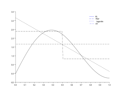
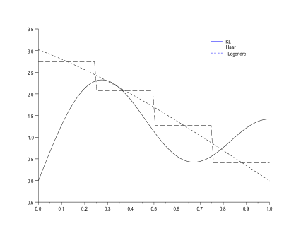
We set the optimal product quantizer at level which corresponds to the optimal decomposition , , , for the problem (14) (see [16] for more details). The number of Monte-Carlo simulations is 100,000 in every case. Note once again that for each basis and each value of the dimension , the prices and the variances are computed using the same pseudo-random number generator initialized with the same seed. In Figure 1 are depicted the optimal variance reducer when the minimization of is carried out on for several values of in the different basis mentioned above.
| Basis | m | Price MC | Variance MC | Price QIS | Variance QIS |
|---|---|---|---|---|---|
| Constant | 1 | 7.112 | 293.98 | 7.006 | 79.07 |
| Legendre | 2 | 7.179 | 296.52 | 7.062 | 22.46 |
| (ShLeg) | 4 | 7.033 | 290.71 | 7.093 | 22.17 |
| 8 | 7.180 | 300.72 | 7.096 | 22.25 | |
| Karhunen-Loève | 2 | 7.102 | 296.91 | 7.043 | 83.81 |
| (KL) | 4 | 7.066 | 295.76 | 7.034 | 74.31 |
| 8 | 7.082 | 290.51 | 7.096 | 37.69 | |
| Haar | 2 | 7.104 | 293.13 | 7.035 | 33.14 |
| (Haar) | 4 | 7.110 | 297.77 | 7.074 | 25.07 |
| 8 | 7.136 | 299.64 | 7.065 | 23.17 |

Local-Volatility Model: Now, we consider the same payoff function in a local volatility model (inspired by the CEV model) defined by
| (38) |
with , , and . For numerics, the solution of the ODE given by (15) is approximated by a sixth order Runge-Kutta scheme. The number of Monte-Carlo simulations is 50,000 in every case. The numerical results are summarized in Table 4.
| Basis | m | Price MC | Variance MC | Price QIS | Variance QIS |
|---|---|---|---|---|---|
| Constant | 1 | 6.635 | 205.69 | 6.681 | 58.63 |
| Legendre | 2 | 6.646 | 204.84 | 6.619 | 16.94 |
| (ShLeg) | 4 | 6.593 | 206.52 | 6.661 | 16.84 |
| 8 | 6.537 | 203.39 | 6.627 | 17.29 | |
| Karhunen-Loève | 2 | 6.562 | 203.73 | 6.620 | 66.55 |
| (KL) | 4 | 6.627 | 205.24 | 6.578 | 53.25 |
| 8 | 6.700 | 207.31 | 6.637 | 32.61 | |
| Haar | 2 | 6.583 | 204.65 | 6.651 | 26.06 |
| (Haar) | 4 | 6.535 | 203.09 | 6.669 | 18.82 |
| 8 | 6.679 | 206.39 | 6.656 | 17.48 |
Schwartz’s Model: Again we consider the same payoff function in the Schwartz model with , , , , . The number of Monte-Carlo simulation is 100,000 in every case. The numerical results are summarized in Table 5. Note that since the spot price can be written
Hence, to quantize the diffusion , we just have to obtain a (rate optimal) -product quantizer of the centered Ornstein-Uhlenbeck process . It is given by
where is the unique optimal -quantizer of the normal distribution, , . Consequently we save computation time since we don’t need to devise a Runge-Kutta scheme.
| Basis | m | Price MC | Variance MC | Price QIS | Variance QIS |
|---|---|---|---|---|---|
| Constant | 1 | 5.012 | 173.59 | 4.905 | 40.07 |
| Legendre | 2 | 5.029 | 173.80 | 4.952 | 11.74 |
| (ShLeg) | 4 | 4.980 | 170.77 | 4.978 | 11.78 |
| 8 | 5.091 | 180.02 | 4.962 | 12.00 | |
| Karhunen-Loève | 2 | 4.928 | 171.54 | 4.960 | 44.55 |
| (KL) | 4 | 4.974 | 171.92 | 4.956 | 39.48 |
| 8 | 4.980 | 171.64 | 4.961 | 21.50 | |
| Haar | 2 | 4.999 | 173.55 | 4.944 | 17.47 |
| (Haar) | 4 | 5.027 | 175.04 | 4.949 | 13.28 |
| 8 | 4.932 | 169.83 | 4.970 | 12.28 |
Down & In Call option: We consider an Down & In Call option of strike and barrier . This option is activated when the underlying process moves down and hits the barrier . The payoff function at maturity T is defined by
A standard approach to price the option is to consider the continuous Euler scheme of step obtained by extrapolation of the Brownian Motion between two instants of discretization. For every , we can write
By preconditioning,
where is the probability of non exit of some brownian bridge. Using the law of the brownian bridge (see for example [9]), we can write
| (39) | |||
| (43) |
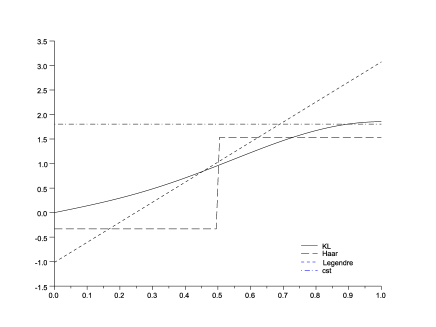
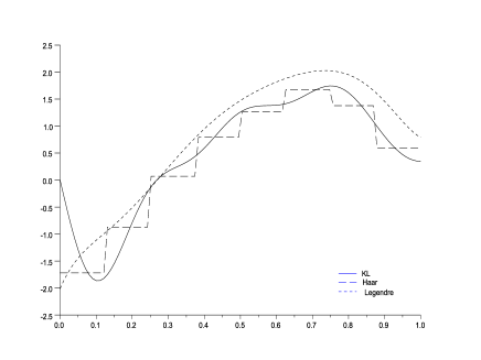
Hence, we run our algorithm with this modified payoff function: . We set the number of steps . In the following simulations, we consider the local volatility model (38) and the classical Black-Scholes model. The results are summarized in Table 6 and Table 7. In Figure 2 are depicted the optimal variance reducer for the local volatility model. Our numerical results illustrate the effectiveness of our Newton-Raphson’s IS algorithm. In this example, the computation time needed to achieve a given precision is divided by a factor 8 in comparison with the crude Monte Carlo estimator.
| Basis | m | Price MC | Variance MC | Price QIS | Variance QIS |
|---|---|---|---|---|---|
| Constant | 1 | 0.684 | 25.80 | 0.673 | 15.33 |
| Legendre | 2 | 0.711 | 27.92 | 0.662 | 4.58 |
| (ShLeg) | 4 | 0.683 | 25.66 | 0.684 | 3.46 |
| 8 | 0.686 | 26.59 | 0.685 | 3.35 | |
| Karhunen-Loève | 2 | 0.680 | 25.38 | 0.696 | 5.22 |
| (KL) | 4 | 0.702 | 26.39 | 0.683 | 6.53 |
| 8 | 0.687 | 26.39 | 0.688 | 5.80 | |
| Haar | 2 | 0.648 | 24.90 | 0.673 | 8.15 |
| (Haar) | 4 | 0.671 | 25.15 | 0.692 | 5.46 |
| 8 | 0.709 | 30.17 | 0.700 | 5.29 |

| Basis | m | Price MC | Variance MC | Price QIS | Variance QIS |
|---|---|---|---|---|---|
| Constant | 1 | 0.481 | 21.76 | 0.467 | 8.62 |
| Legendre | 2 | 0.455 | 19.25 | 0.469 | 3.54 |
| (ShLeg) | 4 | 0.474 | 21.03 | 0.477 | 3.43 |
| 8 | 0.451 | 19.96 | 0.470 | 3.39 | |
| Karhunen-Loève | 2 | 0.466 | 21.36 | 0.459 | 5.51 |
| (KL) | 4 | 0.470 | 22.37 | 0.471 | 5.78 |
| 8 | 0.462 | 21.93 | 0.465 | 5.20 | |
| Haar | 2 | 0.471 | 22.16 | 0.473 | 7.38 |
| (Haar) | 4 | 0.469 | 22.08 | 0.464 | 5.03 |
| 8 | 0.470 | 21.09 | 0.476 | 5.26 |
References
- [1] B. Arouna. Adaptative monte carlo method, a variance reduction technique. Monte Carlo Methods Applications, 10(1):1–24, 2004.
- [2] B. Arouna. Robbins monro algorithms and variance reduction in finance. Journal of Computational Finance, 7:35–61, Winter 2003/04.
- [3] H. F. Chen, G. Lei, and A. J. Gao. Convergence and robustness of the robbins-monro algorithm truncated at randomly varying bounds. Stochastic Processes & Their Applications, 27:217–231, 1987.
- [4] H. F. Chen and Y. M. Zhu. Stochastic approximation procedures with randomly varying truncations. Scientia Sinica Series, 29(9):914–926, 1986.
- [5] D. Dufresne and F. J. Vazquez-Abad. Accelerated simulation for pricing asian options. Proceedings of the 1998 Winter Simulation Conference, pages 1493–1500, 1998.
- [6] M. C. Fu and Y. Su. Optimal importance sampling in securities pricing. Journal of Computational Finance, 5(4):27–50, 2000.
- [7] P. Glasserman, P. Heidelberger, and P. Shahabuddin. Asymptotically optimal importance sampling and stratification for pricing path-dependent options. Mathematical Finance, 9:117–152, 1999.
- [8] P. W. Glynn and L. Iglehart, D. Importance sampling for stochastic simulations. Management Science, 35:1367–1389, 1989.
- [9] E. Gobet. Weak approximation of killed diffusion using euler schemes. Stochastic Processes & Their Applications, 87(2):167–197, 2000.
- [10] S. Graf and H. Luschgy. Foundations of Quantization for Probability Distributions. Lect. Notes in Math. 1730,. Springer, 2000.
- [11] B. Jourdain. Adaptive variance reduction techniques in finance. Advanced Financial Modelling, pages 205–222, 2009.
- [12] B. Jourdain and J. Lelong. Robust adaptive importance sampling for normal vectors. Annals of Applied Probability, 19(5):1687–1718, 2009.
- [13] J. Lelong. Algorithmes stochastiques et Options parisiennes. PhD thesis, ENPC, 2007.
- [14] J. Lelong. Almost sure convergence of randomly truncated stochastic algorithms under verifiable conditions. Statistics & Probability Letters, 78(16), 2008.
- [15] V. Lemaire and G. Pagès. Unconstrained recursive importance sampling. Annals of Applied Probability, 20:1029–1067, 2010.
- [16] H. Luschgy and G. Pagès. Functional quantization of gaussian processes. Journal of Functional Analysis, 196:486–531, 2002.
- [17] H. Luschgy and G. Pagès. Functional quantization of a class of brownian diffusions: A constructive approach. Stochastic Processes & Their Applications, 116:310–336, 2006.
- [18] G. Pagès. A space quantization method for numerical integration. Journal of Computational and Applied Mathematics, 89:1–38, 1998.
- [19] G. Pagès. Quadratic optimal functional quantization of stochastic processes and numerical applications (plenary conference). Proceedings of MCQMC 06, Springer-Verlag:103–147, 2007.
- [20] G. Pagès and J. Printems. Functional quantization for numerics with an application to option pricing. Monte Carlo Methods an Applications, 11(4):407–446, 2005.
- [21] L. Rogers and D. Williams. Diffusions, Markov Processes and Martingales. Cambridge Mathematical Library, 1986.
- [22] E. S. Schwartz. The stochastic behavior of commodity prices: Implications for valuation and hedging. Journal of Finance, 52(3):923–973, 1997.