Do X-ray dark or underluminous galaxy clusters exist?

We study the X-ray properties of a color-selected sample of clusters at $0.1<z<0.3$, to quantify the real aboundance of the population of X-ray dark or underluminous clusters and at the same time the spurious detection contamination level of color-selected cluster catalogs. Starting from a local sample of color-selected clusters, we restrict our attention to those with sufficiently deep X-ray observations to probe their X-ray luminosity down to very faint values and without introducing any X-ray bias. This allowed us to have an X-ray- unbiased sample of 33 clusters to measure the L_X-richness relation. Swift 1.4 Ms X-ray observations show that at least 89 % of the color-detected clusters are real objects with a potential well deep enough to heat and retain an intracluster medium. The percentage rises to 94 % when one includes the single spectroscopically confirmed color-selected cluster whose X-ray emission is not secured. Looking at our results from the opposite perspective, the percentage of X-ray dark clusters among color-selected clusters is very low: at most about 11 per cent (at 90 % confidence). Supplementing our data with those from literature, we conclude that X-ray- and color- cluster surveys sample the same population and consequently that, in this regard we can safely use clusters selected with any of the two methods for cosmological purposes. This is an essential and promising piece of information for upcoming surveys in both the optical/IR (DES, EUCLID) and X-ray (eRosita). Richness correlates with X-ray luminosity with a large scatter, $0.51\pm 0.08$ ($0.44\pm 0.07$) dex in $lgL_{X}$ at a given richness, when $L_{x}$ is measured in a 500 (1070) kpc aperture. We release data and software to estimate the X-ray flux, or its upper limit, of a source with over-Poisson background fluctuations (found in this work to be $\sim 20$ % on cluster angular scales) and to fit X-ray luminosity vs richness if there is an intrinsic scatter. These Bayesian applications rigorously account for boundaries (e.g. the X-ray luminosity and the richness cannot be negative).

1 Introduction

Statistical studies of galaxy cluster samples are important for cosmological studies. The effectiveness of cluster samples critically depends on several factors, among which is the accuracy of the knowledge of the selection function and biases. Cluster samples suited for these studies are collected by means of surveys in optical, X-ray, or radio energy bands. Albeit Sunyaev-Zeldovich surveys are now producing samples useful for cosmological purposes, currently the most efficient methods to compile cluster catalogs for cosmological purposes are still based on optical and X-ray data. Indeed, in the future the two most promising telescopes in this field seem to be in the X-ray (eRosita) and in the optical (e.g. DES).

A critical problem for the use of clusters for cosmological studies is whether optical and X-ray surveys provide fair samples of the dark matter halo mass distribution predicted by the perturbation evolution theories or, equivalently, how far the selection biases in these surveys are known and under control. An important piece of information can be provided by the relation between the optical richness ($n200$) and the X-ray luminosity ($L_{X}$), which are the fundamental parameters for cluster detection and are, at the same time, useful mass proxies. This relation has been previously measured by studying the X-ray properties of large optically selected cluster samples and it is usually parametrized by a power law with a (large) intrinsic scatter (Donahue et al. 2001; Gilbank et al. 2004; Rykoff et al. 2008). The amplitude of the $L_{X}$ scatter is commonly explained by the wide range in the dynamical state of the clusters and by the presence of cooling gas, whereas from the optical point of view, the scatter can be ascribed to projection effects or different efficiencies in the galaxy formation (Gilbank et al. 2004).

The existence of an X-ray dark or underluminous, physically distinct population, whose X-ray luminosity is much lower than expected from their optical richness has been also invoked several times in literature. The large differences in X-ray and optical properties of these clusters have been explained by some extreme feedback mechanism (e.g. Castellano et al 2011). Recently, Balogh et al. (2011) studied a mass-selected sample of 18 moderatly massive (3-6 $10^{14}\ M_{\sun}$) nearby (z $<0.1$) clusters and found a bimodality in ICM properties, with a higlhly significant part of X-ray underluminous or dark objects ($\sim$30%). Therefore, an accurate measurement of the $L_{X}-$richness relation and its scatter is surely useful for a better understanding of the selection biases at different wavelengths and, at the same time, to probe the cluster non-gravitational physics and the very existence of X-ray dark or underluminous clusters.

In this work, we study of the X-ray properties and the $L_{X}$-richness relation relation of a small and well-controlled optical sample. Previous works (Donahue et al. 2001; Gilbank et al. 2004; Rykoff et al. 2008) assembled extensive cluster optical catalogs and studied their X-ray properties using the ROSAT shallow observations, mostly the Rosat All Sky Survey. Their use of shallow X-ray data (in the cluster rest-frame) resulted in a large number of almost uninformative upper limits, only ruling out that the observed cluster has a flux much brighter than other similar clusters of the same richness and which is of little use in ascertaining the existence of dark or underluminous clusters. Some of these works (e.g. Rykoff et al. 2008) are also affected by some systematics such as point-source contamination and centring biases. Here we overcome these limitations through deep X-ray observations of a well-controlled optically selected cluster sample whose depth is appropriate to find an X-ray dark population, if this exist.

In Sec. 2 we describe the sample selection; in Secs. 3 and 4 we describe the optical and X-ray data analysis. In Section 5 we describe the fit procedure we used to parametrize the $L_{X}-$richness relation. In Section 6 we revisit previous statements about the existence of underluminous clusters. In sec. 7 we briefly discuss our results. We summarize and conclude our work in Section 8. Throughout this paper we assume $\Omega_{M}=0.3$, $\Omega_{\Lambda}=0.7$ and $H_{0}=70$ km s^-1 Mpc^-1. For the statistical analysis, we adopt a Bayesian framework with uniform priors, unless otherwise stated.

2 Sample selection

We start from the maxBCG cluster catalog (Koester et al. 2007), which is an optically selected, quasi-volume-limited sample of clusters with $0.1<z<0.3$, with very accurate photometric redshifts ($\delta z\sim 0.01$).

We searched for all Swift X-Ray Telescope (XRT hereafter) observations within 8 arcmin from any maxBCG cluster and with an exposure time longer than 3 ks. This yielded 180 observations out of 14000 in the Swift archive at the start of this work.

We restricted our analysis to the clusters with high-quality X-ray observations. We keep those, of the 180 selected clusters, whose 3$\sigma$ flux limit is at least 30 times fainter than the expected X-ray cluster flux. We calculated the $3\sigma$ flux limit (for a point-like source) as in Moretti et al. (2007) and the expected X-ray flux assuming the $L_{X}-n200$ relation reported in Rykoff et al. (2008). This filter can be expressed by

$$\log f_{lim}<42.22+1.82\log\frac{n200}{40}-d_{L}^{2},$$ (1)

where the flux limit is expressed in erg s^-1 cm^-2 and $d_{L}$ is the cluster luminosity distance in cm. This selection is such that an average cluster of a given richness $n200$ is very well detectable in X-ray and allows us to exclude most uninformative upper limits. For example, the poorest cluster cataloged in maxBCG catalog (richness $n200=10$), at the typical redshift of our sample, $z=0.2$, is included in the sample only if it has been observed for at least 15 ks with the Swift XRT, corresponding to a $3\sigma$ flux limit of 2 10^-14erg s^-1 cm^-2. Equation 1 leaves us with 43 clusters. We emphasize that a cluster was kept or removed from the sample independently of its own $L_{X}$ (in this phase, X-ray data were not even downloaded), which is essential to avoid X-ray biases, as discussed in Sec. 6.

In the XRT archive we found three clusters, MS1006+1202, MS1455.0+232 and Abell 1835, which are the target of the observations. To search for underluminous clusters they are not useful, because they are known to be X-ray-bright sources, and leaving them in the sample would introduce a bias in the $L_{X}-$richness relation. Therefore we removed them from the statistical sample, but we kept them in tables and figures.

Three more clusters are aligned with an unrelated bright point X-ray sources, making the measurement of the cluster X-ray emission useless for our purposes. We discarded them. Two more clusters fall too near to the Swift XRT field-of-view boundary to make the X-ray data reliable. We discarded these as well. Finally, two maxBCG clusters are (or might be) multiple detections of clusters already present in the maxBCG catalog. To avoid any ambiguity, we also discarded these, which left us with a final sample of 33 (+3) clusters.

Again we stress that these selections do not introduce any selection effect on the X-ray axis: the cluster X-ray flux is not used, directly or indirectly, to decide if the cluster has to be kept in the sample. The final cluster sample is formed by either serendipitously observed clusters (in the field of a source at a fairly different redshift), or, in 50 % of the cases, belong to our own Swift observational program targeting all rich maxBCG clusters.

Table 1: Observed galaxy counts, solid angle ratios, and cluster masses.

ID	ra	dec	$obsn(<1.43)$	$obsgaltot$	$obsgalbkg$	$Cgal$	$n200$	$lgM200$	other IDs
	(J2000)
(1)	(2)	(3)	(4)	(5)	(6)	(7)	(8)	(9)	(10)
1	125.171	31.953	29.3	25	61	9.95	$20^{+5}_{-5}$	$14.28\pm 0.29$
2	139.148	63.803	50.6	60	29	2.52	$49^{+7}_{-8}$	$14.50\pm 0.28$
3	145.511	8.959	83.8	115	73	3.78	$96^{+11}_{-11}$	$14.67\pm 0.29$	Abell 854 (1.3’)
4*	152.199	11.799	70.1	95	142	6.22	$73^{+8}_{-11}$	$14.60\pm 0.28$	MS1006+1202
6	154.152	24.801	60.2	68	29	4.00	$61^{+8}_{-8}$	$14.55\pm 0.28$	Abell 964 (0.2’)
7	156.988	10.579	57.4	68	18	1.70	$58^{+7}_{-10}$	$14.54\pm 0.28$
9	177.532	57.151	6.7	4	19	20.33	$4^{+1}_{-3}$	$13.86\pm 0.37$
10	177.950	37.258	55.1	72	62	3.85	$57^{+8}_{-10}$	$14.55\pm 0.28$
11	183.997	35.717	7.2	7	39	34.20	$7^{+2}_{-3}$	$14.01\pm 0.33$
12	184.066	35.520	16.4	13	120	28.95	$10^{+3}_{-4}$	$14.10\pm 0.32$
13	184.117	35.639	38.7	41	104	12.52	$33^{+5}_{-8}$	$14.41\pm 0.28$	Abell 1738 (0.6’)
16	201.297	57.600	63.2	81	29	1.75	$65^{+9}_{-10}$	$14.57\pm 0.28$	Abell 1744 (1.4’)
17	201.457	59.330	58.0	64	22	3.62	$59^{+8}_{-9}$	$14.56\pm 0.28$
19	211.869	27.821	49.7	53	45	4.73	$44^{+6}_{-9}$	$14.48\pm 0.29$	Abell 1861 (0.6’)
20	217.778	25.634	45.9	48	11	2.01	$43^{+7}_{-8}$	$14.47\pm 0.28$
21*	224.313	22.342	51.1	60	86	9.07	$51^{+7}_{-9}$	$14.52\pm 0.29$	MS1455.0+232
23	228.214	14.318	69.9	89	46	3.60	$77^{+10}_{-9}$	$14.61\pm 0.29$	Abell 2044 (0.3’)
24	229.075	0.089	58.0	67	21	2.31	$58^{+7}_{-9}$	$14.55\pm 0.28$	Abell 2050 (1.1’)
25	233.265	-0.771	61.5	76	32	3.48	$67^{+8}_{-10}$	$14.59\pm 0.28$
26	233.840	37.396	83.6	114	33	2.01	$98^{+12}_{-10}$	$14.68\pm 0.29$
27	245.254	25.772	43.9	48	65	7.41	$40^{+7}_{-8}$	$14.45\pm 0.29$
28	250.661	27.444	36.6	46	38	3.36	$35^{+7}_{-7}$	$14.42\pm 0.28$
29	253.061	44.823	74.3	95	41	3.10	$83^{+9}_{-10}$	$14.63\pm 0.28$
30	27.115	14.038	29.3	27	18	5.24	$24^{+4}_{-6}$	$14.33\pm 0.30$
31	328.925	12.525	52.1	59	39	5.51	$53^{+6}_{-9}$	$14.52\pm 0.28$
32	140.964	59.512	41.5	47	50	7.04	$41^{+7}_{-7}$	$14.46\pm 0.29$
33	141.833	30.232	23.5	23	172	28.64	$18^{+4}_{-6}$	$14.26\pm 0.30$
34	168.213	53.856	41.3	45	43	8.30	$41^{+6}_{-8}$	$14.46\pm 0.28$
35	179.130	54.361	19.3	15	80	38.45	$14^{+3}_{-4}$	$14.19\pm 0.29$
36	180.201	-1.188	16.4	8	10	8.05	$8^{+2}_{-4}$	$14.03\pm 0.32$
37	203.754	58.719	29.6	32	27	7.13	$29^{+4}_{-7}$	$14.37\pm 0.28$
38*	210.258	2.878	127.6	238	115	3.28	$204^{+16}_{-16}$	$14.85\pm 0.31$	Abell 1835
39	211.664	27.600	24.9	21	101	19.48	$17^{+4}_{-5}$	$14.23\pm 0.29$
40	217.705	28.153	20.8	17	39	11.73	$15^{+4}_{-4}$	$14.20\pm 0.29$
42	319.704	0.560	81.7	104	87	5.50	$89^{+10}_{-11}$	$14.65\pm 0.29$
43	354.416	0.271	89.5	139	124	5.37	$117^{+11}_{-13}$	$14.73\pm 0.30$	Abell 2631 (1.4’)

Objects with an ID with an asterisc are not part of the statistical sample, because they are X-ray selected.

3 Cluster center, richness, mass

We started from the maxBCG catalog to improve the center and richness of our clusters.

The maxBCG catalog reports the coordinates of the brightest galaxy (BCG) in the region as the cluster center. In 10 cases (# 3, 4, 7, 12, 19, 21, 23, 34, 37, 38), the BCG has been mis-identified in the maxBCG catalog, and the quoted cluster center is offset by both the peak of the galaxy density and by the X-ray emission barycenter (which is centered on the galaxy overdensity, see Sec 4) by more than 30 arcsec. Therefore, we updated the cluster center. We note that the fraction of miscentered clusters, $0.28\pm 0.07$, derived from our observations of 10 offset in a sample of 33, agrees with the rough expectations based on simulations (Johnston et al. 2007; Hilbert & White 2010). We emphasize that both the value and the error of this fraction are essential parameters for estimating cosmology parameters (Hilbert & White 2010) or for forecasting their precision in future surveys (Oguri & Takada 2010) using galaxy clusters. Up to now, a rough estimate for the value was taken, and no error on it was considered. The values directly measured for the first time here on real data allow future analyses to provide more realistic estimates.

We derived the cluster richness, $n200$, using the Sloan Digital Sky Survey (hereafter SDSS) $6^{th}$ data release (Adelman-McCarthy et al., 2008), strictly following the Andreon & Hurn (2010) procedure, which rigorously accounts for the finite sample size, uncertainties, and existence of boundaries (e.g. clusters galaxies do not come in negative units, while the usual total minus background difference may be negative because of Poisson fluctuations). We counted the net number of red galaxies within $r_{200}$. This radius is estimated from the net number of red galaxies within $1.43$ Mpc from the cluster center, $obsn(<1.43)$, using equation 18 in Andreon & Hurn (2010), which calibrates this relation with a sample of 54 clusters with kwown $r_{200}$.

Moreover, we used the Andreon & Hurn (2010) measured richness–mass scaling to estimate the masses of our clusters. The quoted mass uncertainty accounts for a number of error sources including the larger calibration uncertainty at the extremes of the richness range, as detailed in Andreon & Hurn (2010). This point has relevance for the richest cluster of our sample, # 38, which has a larger mass error because in the calibrating sample only few clusters are as rich as it is. At the other richness extreme, the error of the poorest cluster in our sample, #9, accounts for the extrapolation in going from the range where the richness-mass is well calibrated, from seven galaxies on, to its richness, about four galaxies. The model is described in detail in Andreon & Hurn (2010), who also give its coding in a user-friendly way.

Table 1 lists the results of the optical analysis. Column 1 lists the cluster id; column 2 and 3 list updated coordinates; column 4 lists the net observed number of galaxies in the cluster line-of-sight within an aperture of 1.43 Mpc, $obsn(<1.43)$; column 5 lists the observed number of galaxies in the cluster line of sight within $r_{200}$, $obsgaltot_{i}$; column 6 gives the observed number of galaxies in the background line-of-sight $obsgalbkg_{i}$; column 7 lists the ratio between the cluster and background solid angles, $Cgal$; column 8 gives the cluster richness (posterior mean and highest posterior 68 % interval); column 9 gives the inferred mass (posterior mean and standard deviation), on a log scale in solar mass units. Finally, column 10 lists other known identifications of the studied clusters when their reported coordinates is within 1.5 arcmin from the center determined by us. The angular offset is reported in parenthesis.

Figure 1 shows the distribution in mass of clusters in our sample: most of them are in the range 1 to 5 $10^{14}$ solar masses, and all are included in the range $0.6$ to $8$ $10^{14}$ solar masses.

Figure 1: Distribution of cluster masses.

Figure 2: Comparison of the richness as determined by us (ordinate) and in the maxBCG catalog. Open points marks miscentered clusters in the maxBCG catalog. There is no error on the abscissa because none is listed in the maxBCG catalog.

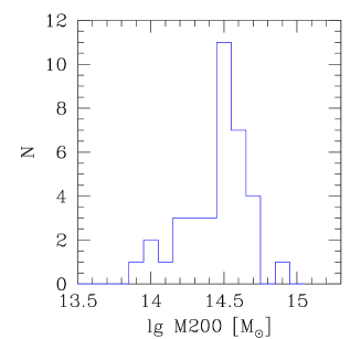
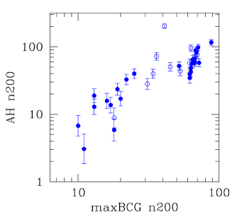
Figure 2 compares the Koester et al. (2007) and our measurements of richness. There is no errorbar in Figure 2 on maxBCG richness because none is listed in their catalog. Figure 2 shows that our sample explores a richness range that goes from the richest (maxBCG richness $\sim 80$) to the poorest (maxBCG richness $10$) clusters in the $0.1<z<0.3$ volume (and in the SDSS area). The two richness estimates broadly agree, although they were derived in slightly different ways: a) Koester et al. count galaxies in different color and luminosity ranges and in different filters; b) we account for background galaxies, whereas Koester et al. do not; c) we adopt different centers (in 30 % of the cases) and also $r_{200}$ values (Koester et al. count galaxies within a radius, unfortunately named $r_{200}$, which is on average $2r_{200}$, e.g. Sheldon et al. 2009; Becker et al. 2007; Johnston et al. 2007). Therefore, it is not surprising that a scatter is present between the two richnesses. The outlier point in Fig. 2 (the point with highest ordinate) is cluster #38, and it is one of those that have a wrong maxBCG estimate of the cluster center. In particular, the area explored by maxBCG (i.e. the circle centered on their center and of radius given by their $r_{200}$) misses about half the cluster.

Figure 3: Redshift dependence of richness residuals. Open points indicate miscentered clusters in the maxBCG catalog. Error bars only consider errors on our richness estimate, because there is no such measurement for the maxBCG.

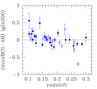
Figure 3 compares residuals between Koester et al. (2007, maxBCG) and our (AH) richnesses vs redshift. There is a small but clear trend with redshift, in the sense that maxBCG richnesses are underestimated at high redshift. Indeed, residuals tend to be positive for the lower half of the redshift range and negative for the upper half. The redshift dependency of the maxBCG richness has already been indirectly pointed out (Reyes et al. 2008, Rykoff et al. 2008; Becker et al. 2007; Rozo et al. 2009). By directly comparing two richness estimates, Figure 3 confirms that the maxBCG richness is redshift-dependent. A redshift trend introduces a systematic bias on the mass estimate and therefore on estimates of cosmological parameters.

Figure 4: Montage of the SWIFT XRT [0.5-2] keV images of clusters in our sample, convolved with a Gaussian kernel with $\sigma=18$ arcsec. The ruler indicates 1 arcmin. North is up, east is to the left. The cluster is marked by a green circle. Red circles mark other sources masked in our analysis.

4 X-ray data

The X-ray telescope (XRT) on board the Swift satellite (Gehrels et al. 2004) uses a Wolter I mirror set, originally designed for the JET-X telescope (Citterio et al. 1994), to focus X-rays (0.2-10 keV) onto a XMM-Newton/EPIC MOS CCD detector (Burrows et al. 2005). The effective area of the telescope ($\sim$ 120 cm² at 1.5 keV) is $\sim$ 3.5 smaller than 1 XMM-Newton MOS module. The PSF, similar to XMM, is characterized by a half-energy-width (HEW) of $\sim$ 18″at 1.5 keV (Moretti et al. 2005).

XRT data were reduced using the standard data reduction procedures as outlined in Moretti et al. (2009). Two of our clusters, # 12 and 34, are angularly not far from a background gamma-ray-burst. In these cases, we removed the first segments of the observations to reduce the noise associated with the bright gamma-ray-burst.

The total SWIFT XRT integration time on our cluster sample is 1.4 Ms.

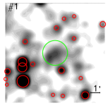
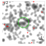
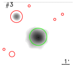
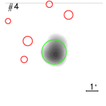
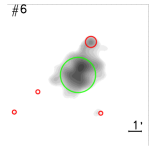
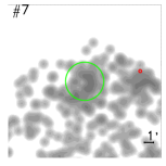
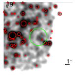
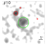
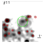
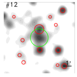
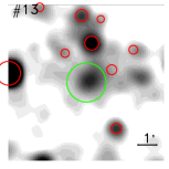
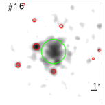
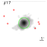
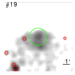
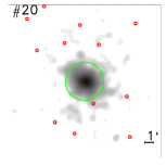
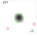
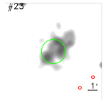
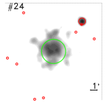
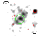
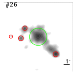
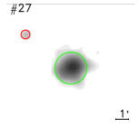
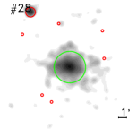
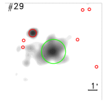
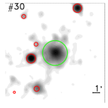
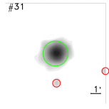
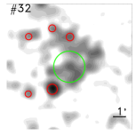
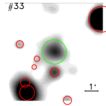
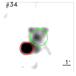
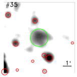
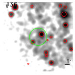
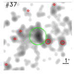
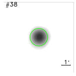
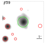
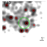
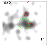
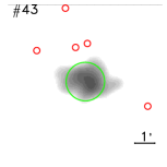
Figure 4 shows [0.5-2] keV images, convolved with a Gaussian kernel with $\sigma=18$ arcsec. The extended X-ray emission of most of them is fairly obvious in this figure.

To estimate the cluster count rate, we measured counts (in the [0.5-2] keV band) in the cluster direction, $obstot_{i}$, within a 500 kpc aperture at the cluster redshift, centered on the revised cluster center. To estimate the background and its fluctuations, we measured the counts in a number ($nbox_{i}$) of regions of the same solid angle as the cluster, spread over the XRT field-of-view.

Figure 5: Expected (red error bars) and observed (black points) spread in background values vs median background value. The upper panel assumes purely Poisson background fluctuations, whereas the lower panel allow a 20 % scatter in the mean background value.

To eliminate the contamination by point sources, we ran the wavedetect CIAO task and we masked X-ray point sources associated to galaxies or optical point objects. This left us with only the signal coming from the ICM. We used exposure maps to calculate the effective exposure time accounting for vignetting, CCD defects, and excised regions.

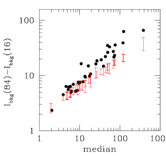
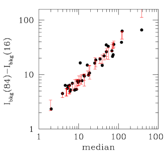
To estimate possible over-Poisson fluctuations of background counts, we computed the 16^th, 50^th (median) and 84^th percentiles of the distribution of background values and from these the spread, $I_{bkg}(84)-I_{bkg}(16)$, plotted in the abscissa of Figure 5. We then computed the same percentiles for a sample of simulated $nbox_{i}$ background values drawn from a Poisson distribution of mean intensity $\mu$. The upper panel of Figure 5 shows that the observed spread (solid points) is larger than the simulated one (error bar, showing the 68 % range of simulated spreads) assuming Poisson fluctuations only. Note that the observed spread is noisy and has a systematic bias because we measured it from a finite number of elements. Noise and systematic are both addressed by our simulation. The lower panel shows simulations that better match the observed spread: we allowed the background to have a 20 % Gaussian fluctuation on the top of the Poisson fluctuations. The agreement between observed and simulated spread is fairly good, and therefore, we allowed 20 % over-Poisson background fluctuation throughout.

Of course, we kept separate data from different pointings in our calculation because we are interested in background variations on cluster angular scales.

To summarize, we found that the $nbox_{i}$ background values scatter more than expected if the only source of background fluctuations were Poisson i.e. we detected over-Poisson fluctuations of background counts consistent with a 20 % amplitude. Some over-Poisson fluctuation is expected (Moretti et al. 2011).

Modeling this term is important for low surface brightness objects whose intensity is heavily affected by a 20 % background variation. In particular, our modeling of the over-Poisson fluctuations of the background is important for the three faintest clusters, #9, 36 and 40, which otherwise would have their luminosity error underestimated by about 0.2 dex.

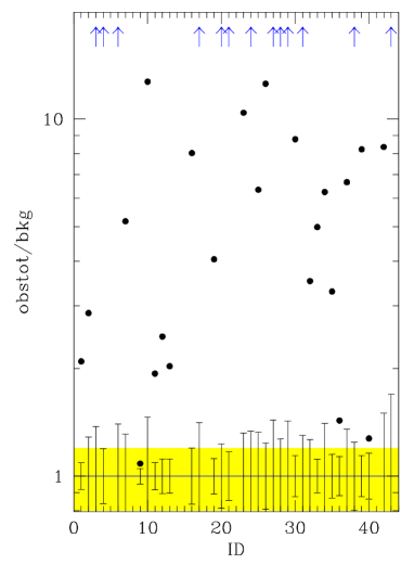
Figure 6 shows X-ray counts in the direction of the clusters in units of the mean background value measured all around them, together with background errors and 20 % over-Poisson fluctuations. All clusters, except #9, display a significant excess of X-ray counts in a 500 kpc aperture. For cluster #9, we measured a flux excess higher than expected Poisson fluctuations, but well consistent with a 20 % background fluctuation. Clusters # 36 and # 40 have also low S/N X-ray counts in the 500 kpc aperture, but their detection is secure adopting an optimized aperture.

Figure 6: X-ray counts in the direction of the clusters (points) in units of the mean background value measured all around them. The error bars indicate heuristic ($\sqrt{n}$) background Poisson fluctations. The (yellow) shading indicates the 20 % over-Poisson fluctations. Thirtenn clusters, indicated by a lower limit, are too bright to fit in this figure.

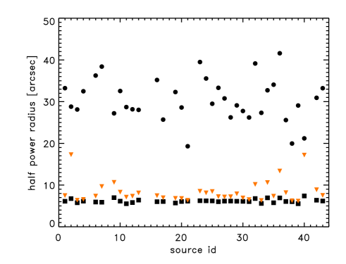
To ascertain the extension of the X-ray emission, we calculated for each cluster the half-power-radius (HPR), defined as the radius enclosing 50% of the fluence within a 1 arcmin (25 pixels) circle radius, which corresponds to the $\sim$ 95% of the PSF encircled energy fraction. We assessed the significance of the extension of each cluster simulating 1000 PSFs with the same counts, the same spectrum and same off-axis angle. To each simulated PSF we added a background, accounting for its whole variance (Poisson and over Poisson). The typical HPR of a point -like source is 3 pixels (7 arcsec) with a distribution tail that mostly depends on the signal-to-noise ratio. Fig. 7 shows that for all the clusters of our sample the HPR lies well beyond the 90^th percentile of the HPR PSF simulation distributions, except # 40, which barely exceeds it. In this case a significance near 100 % is precluded by small number statistics and high allowed (Poisson plus over-Poisson) fluctuations.

Figure 7: Half power radius of clusters (black circle) compared with the $50^{th}$ (square) and $90^{th}$ (orange triangle) percentile of the distribution of PSFs simulated in the same conditions (off-axis, spectrum, counts and background).

We computed the X-ray count rate of the clusters in our sample using the fitting model in Appendix A, which accounts for the Poisson nature of counts, over-Poisson background fluctuations, uncertainty on the mean value of the background, and the existence of boundaries in the data and parameter space. Cluster counts were converted into X-ray luminosities accounting for the exposure map and assuming a thermal spectrum (APEC) of $T=1.5$ keV, 0.3 times the solar value metallicity, at the cluster redshift and the Galactic absorption (Kalberla et al. 2005). We checked that using a $T=3.5$ keV temperature does not alter our conclusions. Figure 8 shows the (posterior) probability distribution of $L_{X}$ for our clusters. Sharp distributions indicate precisely determined $L_{X}$. Note the asymmetry and general non-Gaussian shape of clusters with lower quality determinations of $L_{X}$.

We detail the fitting model in Appendix A in a user-friendly way for computing the flux, and/or its upper limit, of whatever source. Again, the use of this model is particularly important for the faintest elements of our catalog, which are the most interesting cases for the purposes of this work. The fitting model returns physically acceptable values in all situations, including when observed counts in the cluster direction are lower than the average measured background, a situation that occurs, for example, when a faint cluster is on the top of a negative background fluctuation. Returned uncertainties behave as expected: they do not include non-physical (negative) X-ray luminosities and are large when the X-ray flux is low, which is not guaranteed in other approaches (as illustrated in Kraft et al. 1991).

Figure 8: (Posterior) $L_{X}$ probability distribution for clusters in our sample. Curves are offset vertically to improve readibility. Note the non-Gaussian shape (e.g. asymmetry) of the several of them, as also indicated by asymetric errors in Table 2.

Table 2 lists cluster id (column 1), Swift exposure time on source (column 2), total number of photons in the cluster direction, $obstot_{i}$ (column 3), and in the background direction, $obsnbkg_{i}$ (column 4). The latter is measured in a solid angle $nbox_{i}$ times larger. Column 6 gives the number needed to convert counts into X-ray luminosity. Column 7 lists derived X-ray luminosities and their 68 % (highest posterior) intervals.

To summarize, all clusters, except #9, display a significant extended X-ray emission, as shown in Fig 6 & 7. As mentioned, the X-ray emission of cluster #9 is not secured. The X-ray detection of 32 clusters out of 33 implies that the 90 % upper limit fraction of X-ray dark clusters is $0.11$. This number should be read as pessimistic because cluster #9 is likely an X-ray emitting system. Therefore we can infer that X-ray surveys do not systematically miss a significant population of X-ray dark halos, which is an essential assumption for any cosmological use of X-ray cluster surveys such as those that will be performed e-Rosita and, possibly, WFXT.

The fraction of color-detected clusters that are real objects is even higher, 0.935 (at 90 % confidence), because cluster #9, for which our X-ray data provide no compelling evidence, is spectroscopically confirmed. In other words, we find that all color-selected clusters are real (the 90 % upper limit to spurious detection is $0.065$); this is an essential and promising piece of information for incoming surveys as DES or EUCLID.

Our finding of a tight upper limit to the fraction of X-ray dark clusters agrees with the results of Donahue et al. (2001), but offers a more stringent constraint. While up to 75 % of the optically selected clusters in Donahue et al. (2001) might be dark because X-ray undetected, our 90 % upper limit is around 5 to 10 %. We find a tight upper limit because our observation strategy has been tailored to avoid little informative upper limits to the X-ray flux, i.e. values brighter than, or comparable to, the mean $L_{X}$-richness relation.

Our upper limit to the fraction of X-ray dark cluster agrees with the fraction one can derive from the X-ray observations of 13 clusters at much higher redshift, $0.6<z<1.1$ reported in Hicks et al. (2008) and Bignamini et al. (2008). Counting as possibly dark all clusters that do not have a clear X-ray detection, one in our sample and three in theirs, the 90 % upper limit to the fraction of X-ray dark clusters is 11 % in our sample, and 42 % in theirs. The latter value is higher because their sample size is small, only 13 systems, and their X-ray upper limits are little informative.

Table 2: X-ray data

ID	$t_{exp}$	obstot	obsbkg	nbox	C	$\log L_{X}$
						erg s-1
1	125.4	259	4079	33	40.41	$42.52^{0.13}_{-0.06}$
2	4.3	35	269	22	41.49	$42.84^{0.14}_{-0.10}$
3	8.9	457	356	51	41.73	$44.38^{0.02}_{-0.02}$
4*	36.4	1223	1534	57	41.31	$44.38^{0.01}_{-0.01}$
6	5.0	156	325	52	41.77	$43.95^{0.04}_{-0.04}$
7	4.2	53	256	25	41.38	$43.02^{0.08}_{-0.07}$
9	184.1	415	3827	10	39.67	$41.39^{0.48}_{-0.14}$
10	3.8	59	190	41	41.80	$43.54^{0.06}_{-0.06}$
11	94.1	231	4174	35	40.26	$42.29^{0.15}_{-0.06}$
12	121.1	176	4509	63	40.63	$42.64^{0.10}_{-0.06}$
13	149.3	150	4503	61	40.66	$42.53^{0.14}_{-0.07}$
16	10.2	204	330	13	41.04	$43.30^{0.04}_{-0.03}$
17	5.0	296	171	29	41.68	$44.14^{0.03}_{-0.02}$
19	67.7	277	2326	34	40.59	$42.91^{0.05}_{-0.04}$
20	4.4	567	188	10	41.30	$44.04^{0.02}_{-0.02}$
21*	30.1	3522	2133	62	41.38	$44.93^{0.01}_{-0.01}$
23	4.2	101	562	58	41.88	$43.85^{0.05}_{-0.05}$
24	2.1	179	239	27	41.84	$44.07^{0.03}_{-0.03}$
25	5.0	59	400	43	41.74	$43.44^{0.07}_{-0.07}$
26	12.4	223	337	19	41.20	$43.51^{0.03}_{-0.03}$
27	4.5	190	340	65	41.97	$44.24^{0.03}_{-0.03}$
28	4.6	310	190	14	41.43	$43.90^{0.03}_{-0.03}$
29	3.6	101	262	48	41.90	$43.88^{0.05}_{-0.04}$
30	17.4	434	840	17	40.94	$43.52^{0.03}_{-0.02}$
31	9.9	691	396	36	41.60	$44.43^{0.02}_{-0.02}$
32	18.0	49	724	52	41.29	$42.83^{0.10}_{-0.08}$
33	159.3	380	4650	61	40.80	$43.28^{0.04}_{-0.03}$
34	7.8	38	468	77	41.72	$43.23^{0.09}_{-0.08}$
35	89.9	144	2539	58	40.76	$42.76^{0.08}_{-0.05}$
36	26.8	79	828	15	40.59	$41.92^{0.33}_{-0.11}$
37	4.8	53	199	25	41.63	$43.28^{0.08}_{-0.06}$
38*	12.9	3135	1257	76	41.80	$45.29^{0.01}_{-0.01}$
39	81.2	412	3302	66	40.87	$43.43^{0.03}_{-0.03}$
40	27.3	50	1098	28	40.91	$41.94^{0.43}_{-0.13}$
42	6.3	33	387	98	42.13	$43.60^{0.09}_{-0.08}$
43	2.9	96	198	96	42.51	$44.48^{0.05}_{-0.04}$

Objects with an ID with an asterisc are not part of the statistical sample, because they are X-ray selected.

We stress that our conclusion are applicable to color-detected clusters in the local Universe ($0.1<z<0.3$) using a filter pair that brackets the 4000 Å  break, of richness comparable to the clusters listed in the maxBCG catalog ($>10$ galaxies counted as they do, or $\geq 4$ as we do). As just mentioned, there are indications that the same results may hold true at higher redshift.

We note that the fraction of spurious detection that we find in the MaxBCG catalog ($<$ 6.5%) is consistent with the typical contamination level of X-ray and SZ catalogs. For example, 1 in 34 of the REFLEX (i.e. X-ray) selected clusters have subsequently been discovered to be AGNs (Boheringer et al. 2007); a similar fraction of objects are expected to be false positives in the 400d survey (Burenin et al. 2007). Four out of 21 new cluster candidates identified in the Planck ESZ sample are known not to be single clusters and are instead double or triple systems from XMM follow-up observations (Aghanim et al. 2011). Note that both these X-ray and SZ selected samples were subject to attentive scrutiny in the optical prior to publication, whereas our sample of maxBCG clusters were not filtered out by any X-ray data inspection.

5 $L_{X}-$richness relation

As we have said, the 90 % (pessimistic) upper limit fraction of X-ray dark clusters is 11%. We will now to address a finer question, namely whether a significant population of underluminous clusters exists at all. They may, of course, without being dark (at least in principle), and may thus have been counted as X-ray emitters in the previous section. Therefore, we looked for outliers in the regression between richness and X-ray luminosity.

For this regression, our fitting model assumes a linear relation between (the log of) the true richness and true X-ray flux (with some intrinsic scatter), but rather than these true values, we have noisy measurements of both richness and X-ray flux, with noise amplitude different from point to point. We account for the Poisson nature of counts, the non-Poisson nature of X-ray flux and richness, for higher than Poisson fluctuations in the X–ray background and covariance for all modeled quantities. This computation requires the use of the full probability distribution for intervening quantities, not just the point estimates of X-ray flux and richness given in Table 1 and 2. The fitting model is fully described in Appendix B, where we also give its coding. To our best knowledge, this model and the one of in Appendix A have never been published before.

Figure 9: X-ray luminosity-richness scaling. The solid line indicates the mean fitted regression line of $\log L_{X}$, measured within a 500 kpc aperture, on $\log n200$, while the dashed line shows this mean plus or minus the intrinsic scatter $\sigma_{scat}$. The shaded region marks the 68% highest posterior credible interval for the regression. Error bars on the data points represent observed errors for both variables (computed following the usual astronomical practice). The distances between the data and the regression line is partly caused by the measurement error and partly by the intrinsic scatter. The upper abscissa indicates the cluster mass.

Figure 10: Posterior probability distribution for the parameters of the X-ray luminosity-richness scaling. The black jagged histogram shows the posterior as computed by MCMC, marginalized over the other parameters. The red curve is a Gaussian approximation of it. The shaded (yellow) range shows the 95 % highest posterior credible interval. The jagged nature of the histogram is caused by the finite sampling of the posterior.

Figure 11: As Fig 9, but for an $L_{X}$ measured in an aperture of 1070 kpc.

Using the fitting model, we found for our sample of 33 color-selected clusters

$$lgL_{X}=(1.69\pm 0.30)\ (\log n200-1.8)+43.71\pm 0.11\quad.$$ (2)

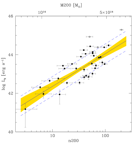
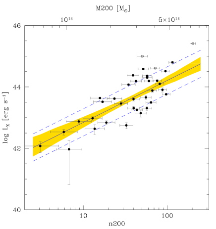
Figure 9 shows the scaling between richness and X-ray luminosity, observed data, the mean scaling (solid line) and its 68% uncertainty (shaded yellow region) and the mean intrinsic scatter (dashed lines) around the mean relation. The $1\sigma_{scatt}$ band is not expected to contain 68% of the data points because of the measurement errors. All points are, however, within twice the intrinsic scatter. The upper abscissa also gives the cluster mass.

Figure 10 shows the posterior probability distribution of the intercept, slope, and intrinsic scatter $\sigma_{scat}$. These probability distributions are reasonably well approximated by Gaussians. The intrinsic $L_{X}$ scatter at a given richness, $\sigma_{scat}=\sigma_{lgL_{X}|\log n200}$, is very large, $0.51\pm 0.08$ dex. In other terms, a whole 1 dex in $L_{X}$ is needed to bracket 68 % of clusters of a given richness.

Figure 9 also shows that the three (out of three) X-ray selected clusters (for this reason not fitted) are much brighter than the mean regression, as expected for X-ray selected objects. Figure 9 shows that the data of cluster # 9 (the object with the lowest $n200$ and an X-ray flux excess higher than the Possion fluctuation, but still consistent with a 20 % background fluctuation) are also compatible with the X-ray luminosity expected for its richness.

Figure 9 allows us to address the question mentioned at the start of this section, whether there is a population of clusters with much lower X-ray luminosity at a given richness or mass, i.e. underluminous. None of them has been found in our sample, because no point is much off from the regression, the farthest one being about 1.5 times the intrinsic scatter. Indeed, the current data allow us to set an upper limit to the fraction of underluminous clusters. Because no outlier is present in a sample of 33, this sets a 90 % upper limit of 0.065.

We used a 500 kpc aperture as a good compromise between the physical dimensions of the cluster and the typical apparent size in our observation. To test the robustness of our results we also measured the relation using an aperture of 1.07 Mpc (adopted by Rykoff et al. 2008). We found

$$lgL_{X}=(1.36\pm 0.26)\ (\log n200-1.8)+43.93\pm 0.10$$ (3)

and an intrinsic scatter of $0.44\pm 0.07$. Fig 11 shows the scaling between richness and X-ray luminosity with this larger aperture. These parameters are consistent with those derived using the small aperture. If anything, the intercept is slightly larger than using a smaller aperture because there is some cluster flux outside $0.5$ Mpc. As in the case of the smaller aperture, there are no outliers and no cluster qualifies itself as underluminous.

Slope and intercept agree with the values reported in Rykoff et al. (2008). Our intrinsic scatter, which formally agreement, is larger than the total scatter they report, even though we expect the contrary because their (total) scatter does not account for point-source contamination, for miscentering (30 % of clusters with wrong coordinates), redshift dependence of their definition of richness, and richness errors. We checked to find a larger scatter also adopting the MaxBCG $n200$ definition. We emphasize that while these observed differences are within the errors, our work gives the first robust measurement of the intrinsic scatter of $L_{X}$ at a given richness, previous attemps (e.g. Rykoff et al. 2008) do not have completely removed all observationally-related effects from its estimate.

6 Do we know any underluminous clusters?

We found no underluminous clusters. However, other works (e.g. Bignamini et al. 2008, Hicks et al. 2008, Castellano et al. 2011, Dietrich et al. 2009, Balogh et al. 2011) do. What is the reason for this? To claim that a cluster is underluminous, it is critical

a) to account for the intrinsic scatter. If none is assumed, a cluster is claimed to be underluminous when instead it is normal, i.e. just one (true) $\sigma_{intr}$ below from the mean relation. Once the intrinsic scatter is allowed, the putative Dietrich et al. (2009) X-ray underluminous cluster becomes a normal cluster.

b) to use a non-biased relation as reference to determine the underluminous nature of a putative cluster. Indeed, if a reference relation is (mis)taken biased-high, one may wrongly classify normal clusters as underluminous. The reference relation may be easily biased as high if the comparison sample is formed by X-ray selected clusters or by an uncontrolled sample, as is now well known from the literature (e.g. for the $L_{X}-T$ relation: Pacaud et al. 2007; Stanek et al. 2006; Nord et al. 2008; Andreon et al. 2011; Andreon & Hurn 2011). The bias occurs when the probability that a cluster is included in the sample depends on its own $L_{X}$. This is the case for an X-ray selected sample, but also for every sample for which there is a selection based on (individual) cluster luminosity, flux or counts, (e.g. at least $n$ photons for a temperature measurement, with $n$ often in the range 200-1000). Indeed, in an X-ray selected sample, the bias comes from the larger Universe volume over which a cluster brighter-than-average at a given richness can be seen compared to fainter-than-average clusters. Therefore, in an X-ray selected sample, at a given richness the upper half of the $L_{X}$ distribution will be more populated than the lower half, biasing high the mean, and underestimating the dispersion (if the effect is not accounted for). A similar bias is also likely present in cluster samples assembled from pointed observations of X–ray selected clusters like the ones built by, amongst others, Ettori et al. (2004) and Branchesi et al. (2007). On the contrary, a purely optically (or color, as in this work) selected sample of clusters does not introduce any bias in the $L_{X}$-richness relation, because the average $L_{X}$ at a given richness will not be biased high (or low).

Bignamini et al. (2008), Hicks et al. (2008) conclude that color-selected clusters are underluminous. Castellano et al. (2011) claim the existence of an underluminous cluster. However, their claim is based on the comparion with a biased-high mean $L_{X}-T$.

Finally, Balogh et al. (2011) asses the X-ray properties of their sample using Chandra or XMM observations for all but two clusters (both undetected in X-ray), and claim the existence of five X-ray underluminous clusters in a sample of 18 of mass in the range considered in our sample. However, a) their X-ray upper limits are all equal irrespective of the cluster redshift, exposure time, or X-ray telescope used (Rosat vs Chandra or XMM); b) four out five of them are within 2 sigma (1 dex) of the mean $L_{X}$-richness relation, not enough to call them underluminous (outlier); c) the authors note that three of the five underluminous clusters, objects 13, 17 and 18, are possibly fake objects (chance projections), not truly existing clusters.

Older claims about the existence of underluminous clusters are rebutted in Andreon et al. (2009). That paper shows that underestimated errors may incorrectly lead to classify a cluster as underluminous even when it agrees with the mean relation, for example when it is, say, 3 (wrong) $\sigma$ below the mean relation.

7 Discussion

The analysis of our sample of 33 clusters at $0.1<z<0.3$ and our revision of the recent literature results presented in Sec 6, joined to our revision of older works in Andreon et al. (2009), confirms that X-ray underluminous clusters are rare enough that we are still looking for an example. Some scenarios of cluster formation predict the existence of underluminous clusters, objects in which the gas has been expelled (e.g. Bower et al. 2008, McCarthy et al. 2011). As we found none in a sample of 33, our 90 % upper limit to this type of objects is $0.065$.

This work, which is based on a color-selected sample of clusters, does not address the fraction of clusters without a red sequence. However, past works have shown the absence of X-ray selected clusters without red galaxies, for example 54 out 54 X-ray selected clusters studied in Andreon & Hurn (2010) have red galaxies and all 32 clusters in Garilli et al. (1996) and in Puddu et al. (2001) of the Einstein Medium Sensitivity Surveys have a red sequence. Overall, the general picture that emerges from this work, when joined to the absence of X-ray selected clusters without red galaxies, is that outliers in the dark (X-ray or low richness) side are quite rare and that the X-ray and color selection sample the same population of objects. This conclusion is supported indeed at much higher redshift by the smaller sample analyzed in Bignamini et al. (2008) and Hicks et al. (2008), in which no believable outliers from the mean relation is found, and by the detection of a red sequence (Andreon et al. 2004; 2005) in all X-ray selected clusters of the XMM-LSS survey (Pierre et al. 2004).

8 Summary and conclusions

We studied the X-ray properties of a color-selected sample of clusters at $0.1<z<0.3$ and we critically discussed previous works claiming the existence of underluminous clusters.

Two important guidelines have been strictly followed in the sample selection. First, the sample has been selected to have sufficiently deep X-ray observations to probe their X luminosity down to very faint values and, second, at the same time we did not use any criterium that depends directly or indirectly on the X luminosity, at a given richness, of the single objects. Our sample consist of 33 clusters that fall in sky regions where deep Swift XRT X-ray observations are available.

Using SDSS data, we refined the cluster centers and richnesses and we estimated cluster masses using richness as mass proxy. These clusters have masses in the range between 5 $10^{13}$ and 8 $10^{14}$ solar masses. This allowed an unbiased measure of the $L_{X}$-n200 relation for a small, but representative, sample of galaxy clusters.

Using 1.4 Ms Swift XRT data, we measured the X-ray luminosity within an aperture of 500 kpc. In these calculations, we accounted for terms usually neglected, such as over-Poisson fluctuations of X-ray background counts, which turned out to be on the order of 20 %, cluster miscentering (i.e. that the cluster center is in 30 % of the cases at a sky location different from what is listed in the catalog), the positively defined nature of measured quantities (richness and X-ray luminosity), etc.

Thirty-two out of our 33 color-selected clusters are obvious X-ray detections. The remaining cluster shows an X-ray excess in the cluster direction compatible with a possible background fluctuation but also with the expected X-ray luminosity of a cluster of the same richness. Therefore, the fraction of X-ray dark clusters (if any of them exist) is low: 11% (at 90 % confidence level).

Since t32 out 33 color-detected clusters are X-ray emitting, then at least 89 % of color-detected clusters are real objects with a potential well deep enough to heat and retain an intracluster medium. Because the system with suggestive, but not compelling evidence of an X-ray emission is spectroscopically confirmed, the fraction of false positive in color-selected searches has most probably an upper limit of 6.5 %. The low contamination of color-selected clusters is a requirement for the use of color-selected clusters for cosmological aims and this work directly shows that this requirement is fulfilled in the mass and redshift ranges considered here.

The quite strict upper limit to the fraction of X-ray dark or underluminous clusters, 6.5 to 11 %, depending on the status of our system without compelling evidence of an X-ray emission, also justifies the widespread use of X-ray selected clusters (e.g. Pacaud et al. 2007), in the sense that X-ray surveys do not systematically miss halos with (red) galaxies inside them. Broadly speaking, X-ray and color (galaxy) cluster searches detect the same population: no X-ray dark cluster is found (in this work and in our revision of other works), and no X-ray selected cluster is found (in other works) not to have red galaxies (of course, in the mass range and in the portion of the Universe volume explored by the considered data).

X-ray luminosity, measured within a 500 (1070) kpc aperture, scales with richness with a proportional factor 1.69 (1.36), with a noticeable scatter, $0.51\pm 0.07$ ($0.44\pm 0.07$) dex. The intrinsic scatter is compatible, but larger, than previously reported scatters. Nevertheless, we emphasize that previous attemps (e.g. Rykoff et al. 2008) do not have completely removed all observational-related effects from the scatter estimate, and thus are not quoting a measurement of scatter entirely related to the object under study, i.e. intrinsic to clusters, but a mix of intrinsic scatter and observer-related effects (such as having no flagged point-sources or having centered the X-ray aperture away from the cluster).

Finally, we found that the observed fraction of miscentered clusters is $0.28\pm 0.07$. This parameter and its uncertainty are required to estimate cosmological parameters or to perform cosmological forecasts using richness as mass proxy.

Our results are very promising for cosmological estimates based on galaxy-detected clusters at least for the redshift and mass ranges considered in this work: surveys as DES or EUCLID will image a large part of the sky, returning color-selected clusters with the same low contamination of X-ray selected clusters (as shown in this work), with a mass proxy of equal quality (Andreon & Hurn 2010), but with an at least 10 times larger sample (Andreon & Hurn 2010). Galaxy-detected clusters are also promising when compared to current SZ-detected clusters: current SZ surveys return one hundred to one thousand fewer clusters than optical searches (e.g. one cluster per 8 to 19 deg², Vanderlinde et al. 2010; Marriage et al. 2011), with a mass proxy that has an observationally determined scatter of about 0.5 dex (Rines et al. 2010), i.e. much worser than $n200$ performances (0.3 dex, Andreon & Hurn 2010). Forecasts specifically for EUCLID will be presented in Trotta et al. (in preparation).

Appendix A Model for the X-ray flux, accounting for over-Poisson background fluctuations

The aim of this section is to present a Bayesian analysis of the X-ray luminosity fitting model. In particular, we wish to acknowledge the uncertainty in all measurements, including the background estimation.

Because of errors, observed and true values are not identical. We call $nclus_{i}$ and $nbkg_{i}$ the true cluster and the true background counts in the studied solid angles. We measured the number of photons in both cluster and background regions, $obstot_{i}$ and $obsbkg_{i}$ respectively, for each of our 36 clusters (i.e. for $i=1,\ldots,36$). The background solid angle is $nbox_{i}$ times larger than the cluster solid angle. We assume a Poisson likelihood for both and that all measurements are conditionally independent.

$$obstot_{i} \sim \mathcal{P}(nclus_{i}+nbkgind_{i}/nbox_{i})$$ (4)

$$obsbkg_{i} \sim \mathcal{P}(nbkg_{i})\quad,$$ (5)

where the symbols $\sim$ reads “is distributed as” and and $\mathcal{P}$ stands for the Poisson distribution.

$nbkgind_{i}$ is allowed to fluctuate by 10 % around the global background value, so that the predicted scatter of background values matches the observed one inside each XRT field:

$$nbkgind_{i} \sim \mathcal{\log N}(ln(nbkg),0.2^{2})\quad,$$ (6)

where the symbol $\mathcal{\log N}$ stands for the lognormal distribution.

We assume uniform priors on cluster and background counts, zero-ed to un-physical values:

$$nclus_{i} \sim \mathcal{U}(0,\infty)$$ (7)

$$nbkg_{i} \sim \mathcal{U}(0,\infty)\quad.$$ (8)

Finally, cluster net counts, $nclus_{i}$, are converted into X-ray luminosities as usual:

$$lgLx_{i}\leftarrow log(nclus_{i})+C_{i}\,$$ (9)

where the arrow symbol reads “take the value of”, and $C_{i}$ is the usual conversion from counts to $L_{x}$.

Eq A1 to A6 find an almost literal translation in JAGS (Plummer 2008), Poisson, normal, lognormal and uniform distributions become dpois, dnorm, dlnorm, dunif, respectively. JAGS, following BUGS (Spiegelhalter et al. 1995), uses precisions, $prec=1/\sigma^{2}$, in place of variances $\sigma^{2}$. Furthermore, it uses neperian logarithms, instead of decimal ones.

This model (set of equations) reads in JAGS:

model
{
for (i in 1:length(obstot)) {
obstot[i] ~ dpois(nclus[i]+nbkgind[i]/nbox[i])
nbkgind[i] ~ dlnorm(log(nbkg[i]),1/0.2/0.2)
obsbkg[i] ~ dpois(nbkg[i])
nbkg[i] ~ dunif(1,1.0E+7)
nclus[i] ~ dunif(0,1.0E+7)
# optional, JAGS is not needed to do it
lgLx[i] <- log(nclus[i])/2.30258 +C[i]
}
}

This model (and code) gives the posterior distribution of the cluster X-ray luminosity, given the observed values of cluster and background counts. Data, posterior mean and (highest posterior) 68 % intervals of the X-ray luminosity are listed in Table 2.

Note that a different prior for cluster and background counts may be more appropriate and valuable in other contexts. In Appendix B we adopt the prior inherited from the cluster richness for the cluster signal.

Appendix B Model for the X-ray luminosity vs richness/mass

The aim of this section is to present a Bayesian analysis of the X-ray luminosity-richness fitting model. In particular, we wish to acknowledge the uncertainty in all measurements, including background estimation. Basically, our model regresses two quantities, each one given by the difference of two Poisson deviates (photons or galaxy counts). We allow the existence of an intrinsic scatter between regressed quantities, and higher than Poisson fluctuations of the X–ray background. In the statistics literature, such a model is know as an “errors-in-variables regression” (Dellaportas & Stephens, 1995). Our model is an extension of the model in Andreon & Hurn (2010), accounting for the different nature of one of the modeled quantities (X-ray luminosity instead of mass) and for the presence of over-Poisson fluctuations.

First of all, because of errors, observed and true values are not identically equal. The variables $n200_{i}$ and $ngalbkg_{i}$ represent the true richness and the true background galaxy counts in the studied solid angles. We measured the number of galaxies in both cluster and control field regions, $obsgaltot_{i}$ and $obsgalbkg_{i}$ respectively, for each of our 33 clusters (i.e. for $i=1,\ldots,33$). We assumed a Poisson likelihood for both and that all measurements are conditionally independent. The ratio between the cluster and control field solid angles, $Cgal_{i}$, is exactly known. In formulae:

$$obsgalbkg_{i} \sim \mathcal{P}(ngalbkg_{i})$$ (10)

$$obsgaltot_{i} \sim \mathcal{P}(ngalbkg_{i}/Cgal_{i}+n200_{i})\quad,$$ (11)

For the X-ray photons a similar construct holds, as detailed in the section above, with eq A4 removed (the prior on $L_{X}$ is inherited from $n200$ and $\sigma_{scatt}$ ones), and eq A6 replaced by

$$nclus_{i}\leftarrow 10^{lgLx_{i}-C_{i}}\quad.$$ (12)

We assume a linear relation between the unobserved $L_{X}$ and $n200$ on the log scale, with intercept $\alpha+44.0$, slope $\beta$ and intrinsic scatter $\sigma_{scat}$:

$$lgLx_{i}\sim\mathcal{N}(\alpha+44+\beta(\log(n200_{i})-1.8),\sigma_{scat}^{2})\quad.$$ (13)

Note that $\log(n200)$ is centered at an average value of 1.8 and $\alpha$ is centred at 44.0, purely for computational advantages in the MCMC algorithm used to fit the model (it speeds up convergence, improves chain mixing, etc.), and that the relation is between true values, not between observed values.

The priors on the slope and the intercept of the regression line in Equation B4 are taken to be quite flat, a zero mean Gaussian with very large variance for $\alpha$ and a Students $t$ distribution with 1 degree of freedom for $\beta$. The latter choice is made to avoid that properties of galaxy clusters depend on humans rules to measure angles (from the x axis anticlockwise or from the y axis clockwise). This agrees with the model choices in Andreon (2006 and later works) but differs from most other works. Our $t$ distribution on $\beta$ is mathematically equivalent to a uniform prior on the angle $b$.

$$\alpha \sim \mathcal{N}(0.0,10^{4})$$ (14)

$$\beta \sim t_{1}\quad.$$ (15)

Finally, we need to specify the prior for the intrinsic scatter, $\sigma_{scat}$, which is positively defined. Following Andreon & Hurn (2010) and Andreon (2010), we impose a quite weak prior information: a Gamma distribution on $1/\sigma_{scat}^{2}$,

$$1/\sigma_{scat}^{2} \sim \Gamma(\epsilon,\epsilon)\quad,$$ (16)

with $\epsilon$ taken to be a very small number.

In JAGS, our model reads

model
{
intrscat <- 1/sqrt(prec.intrscat)
prec.intrscat ~ dgamma(1.0E-5,1.0E-5)
alpha ~ dnorm(0.0,1.0E-4)
beta ~ dt(0,1,1)
for (i in 1:length(obstot)) {
  # modelling X-ray photons
  obstot[i] ~ dpois(nclus[i]+nbkgind[i]/nbox[i])
  nbkgind[i] ~ dlnorm(log(nbkg[i]),1/0.2/0.2)
  obsbkg[i] ~ dpois(nbkg[i])
  nbkg[i] ~ dunif(0,10000)
  # convert nclus in Lx
  nclus[i] <- exp(2.30258*(lgLx[i]-C[i]))
  # modelling galaxy counts
  # n200 term
  obsgalbkg[i] ~ dpois(ngalbkg[i])
  obsgaltot[i] ~ dpois(ngalbkg[i]/Cgal[i]+n200[i])
  n200[i] ~ dunif(1,3000)
  ngalbkg[i] ~ dunif(0,3000)
  # modeling Lx -n200 relation
  z[i] <- alpha+44+beta*(log(n200[i])/2.30258-1.8)
  lgLx[i] ~ dnorm(z[i], prec.intrscat)
  }
}