On the spherical-axial transition in supernova remnants

Abstract

A new law of motion for supernova remnant (SNR) which introduces the quantity of swept matter in the thin layer approximation is introduced. This new law of motion is tested on 10 years observations of SN  1993J . The introduction of an exponential gradient in the surrounding medium allows to model an aspherical expansion. A weakly asymmetric SNR, SN  1006  , and a strongly asymmetric SNR, SN  1987A  , are modeled. In the case of SN  1987A  the three observed rings are simulated.

Keywords  supernovae: general supernovae: individual (SN 1993J ) supernovae: individual (SN 1006 ) supernovae: individual (SN 1987A ) ISM : supernova remnants

1 Introduction

The theoretical study of supernova remnant (SNR) has been focalized on an expression for the law of motion. As an example the Sedov-Taylor expansion predicts $R\propto t^{0.4}$, see see Taylor (1950); Sedov (1959); McCray and Layzer (1987) and the thin layer approximation in the presence of a constant density medium predicts $R\propto t^{0.25}$, see Dyson, J. E. and Williams, D. A. (1997); Dyson (1983); Cantó, Raga, and Adame (2006). The very-long-baseline interferometry (VLBI) observations of SN  1993J (wavelengths of 3.6, 6, and 18 cm) show that $R\,\propto t^{0.82}$ over a 10 year period, see Marcaide et al. (2009). This observational fact does not agree with the current models because the radius of SN  1993J grows slower than the free expansion and faster than the Sedov-Taylor solution, more details for the spherical case can be found in Zaninetti (2011). The SNRs can also be classified at the light of the observed symmetry. A first example is SN  1993J which presented a circular symmetry for 4000 days, see Marcaide et al. (2009). An example of weak departure from the circular symmetry is SN  1006  in which a ratio of 1.2 between maximum and minimum radius has been measured, see Reynolds and Gilmore (1986). An example of axial symmetry is SN  1987A  in which three rings are symmetric in respect to a line which connect the centers, see Tziamtzis et al. (2011). The models cited leave some questions unanswered or only partially answered:

• Is it possible to deduce an equation of motion for an expanding shell assuming that only a fraction of the mass enclosed in the advancing sphere is absorbed in the thin layer?

• Is it possible to model the complex three-dimensional (3D) behavior of the velocity field of the expanding nebula introducing an exponential law for the density ?

• Is it possible to make an evaluation of the reliability of the numerical results on radius and velocity compared to the observed values?

• Can we reproduce complicate features such as equatorial ring + two outer rings in SN  1987A  which are classified as a ”mystery” ?

• Is it possible to build cuts of the model intensity which can be compared with existing observations?

In order to answer these questions, Section 2 describes two observed morphologies of SNRs, Section 3.3 reports a new classical law of motion which introduces the concept of non cubic dependence (NCD) for the mass included in the advancing shell, Section 4 introduces an exponential behavior in the number of particles which models the aspherical expansion, Section 5 applies the law of motion to SN  1987A  and SN  1006  introducing the quality of the simulation, Section 6 reviews the existing situation with the radiative transport equation and Section 7 contains detailed information on how to build an image of the two astrophysical objects here considered.

2 Astrophysical Objects

2.1 A strongly asymmetric SNR , SN  1987A 

The SN  1987A  exploded in the Large Magellanic Cloud in 1987. The distance of this SN is $\approx~{}50~{}kpc$ (163050 $ly$) and a detailed analysis of the distance , $D$ , gives $D=51.4~{}kpc$ Panagia (2005) and $D=50.18~{}kpc$ Mitchell et al. (2002). In the numerical codes we will assume $D=50kpc$ . The observed image is complex and we will follow the nomenclature of Racusin et al. (2009) which distinguish between torus only , torus +2 lobes and torus + 4 lobes. In particular we concentrate on the torus which is characterized by a distance from the center of the tube and the radius of the tube. In Table 2 of Racusin et al. (2009) is reported the relationship between distance of the torus in arcsec and time since the explosion in days.

2.2 A weakly asymmetric SNR, SN  1006 

This SN started to be visible in 1006 AD and actually has a diameter of 12.7 pc, see Strom (1988) . More precisely, on referring to the radio–map of SN  1006  at 1370 MHz by Reynolds and Gilmore (1986), it can be observed that the radius is greatest in the north–east direction. From the radio-map previously mentioned we can extract the following observed radii, $R=6.8~{}pc$ in the polar direction and $R=5.89~{}pc$ in the equatorial direction. Information on the thickness of emitting layers is contained in Bamba et al. (2003) where the Chandra observations (i.e., synchrotron X-rays) from SN  1006  were analyzed. The observations found that sources of non-thermal radiation are likely to be thin sheets with a thickness of about 0.04 pc upstream and 0.2 pc downstream of the surface of maximum emission, which coincide with the locations of Balmer-line optical emission , see Ellison et al. (1994) . The high resolution XMM-Newton Reflection Grating Spectrometer (RGS) spectrum of SN  1006  gives two solutions for the O VII triplet. One gives a shell velocity of   6500 $km/s$ and the second one a shell velocity of 9500 $km/s$, when a distance of 3.4 kpc is adopted ,see Vink (2005).

3 Classical law of motion

3.1 Thermal or non thermal emission?

The synchrotron emission in SNRs is detected from $10^{8}$Hz of radio-astronomy to $10^{19}$Hz of gammaastronomy which means 11 decades in frequency. At the same time some particular effects such as absorption, transition from optically thick to optically thin medium, line emission, and energy decay of radioactive isotopes ( ⁵⁶Ni, ⁵⁶Co) can produce a change in the concavity of the flux versus frequency relationship, see the discussion about Cassiopea A in Section 3.3 of Eriksen et al. (2009). A comparison between non-thermal and thermal emission (luminosity and surface brightness distribution) can be found in Petruk and Beshlei (2007), where it is possible to find some observational tests which allow estimation of parameters characterizing the cosmic ray injection on supernova remnant shocks. At the same time, a technique to isolate the synchrotron from the thermal emission is widely used, as an example see X-limb of SN1006 Katsuda et al. (2010).

3.2 The basic assumptions

The observational dichotomy between thermal and non thermal emission influences the use of temperature in the theoretical models. As an example the Sedov solution is

$$R(t)\approx 0.313\,\sqrt[5]{{\frac{{\it E_{51}}\,{{\it t_{1}}}^{2}}{{\it n_{0}}}}}~{}{pc}\quad,$$ (1)

where $t_{1}$ is the time expressed in years, $E_{51}$, the energy in $10^{51}$ erg and $n_{0}$ is the number density expressed in particles $\mathrm{cm}^{-3}$  (density $\rho=n_{0}$m, where m = 1.4$m_{\mathrm{H}}$), see Sedov (1959); McCray and Layzer (1987); Zaninetti (2011). The spectrum of the emitted radiation depends on the temperature behind the shock front , see for example formula 9.14 in McKee (1987),

$$T=\frac{3}{16}\frac{\mu}{k}v_{\mbox{s}}^{2}\,\,\,K\quad,$$ (2)

where $\mu$ is the mean mass per particle, k the Boltzmann constant and $v_{\mbox{s}}$ the shock velocity expressed in $\mbox{cm~{}sec}^{-1}$. On identifying $v_{s}$ with the velocity derived from Eq. 1 the Sedov solution has the following behavior in temperature

$$T=\frac{3.41\,10^{11}{{\it E_{51}}}^{2/5}}{{{\it n_{0}}}^{2/5}{{\it t_{1}}}^{6/5}}\,\,\,K\quad,$$ (3)

when $\mu$ is the mass of the hydrogen. The Sedov approach cannot be applied to the aspherical case because we do no know the complex volume occupied during the expansion. A numerical approach developed to follow the evolution of the superbubbles first compute the volume occupied during the expansion and then the pressure , see Zaninetti (2004). Conversely the thin layer approximation , see Dyson, J. E. and Williams, D. A. (1997); Dyson (1983), takes in consideration only the swept mass and the velocity is deduced applying the momentum conservation . Due to the absence of the temperature and pressure the thin layer approximation can be classified as a non thermal model.

3.3 The incomplete thin layer approximation

The thin layer approximation with non cubic dependence (NCD) , $p$ , in classical physics assumes that only a fraction of the total mass enclosed in the volume of the expansion accumulates in a thin shell just after the shock front. The global mass between $0$ and $R_{0}$ is $\frac{4}{3}\pi\rho R_{0}^{3}$ where $\rho$ is the density of the ambient medium. The swept mass included in the thin layer which characterizes the expansion is

$$M_{0}=(\frac{4}{3}\pi\rho R_{0}^{3})^{\frac{1}{p}}\quad.$$ (4)

The mass swept between $0$ and $R$ is

$$M=(\frac{4}{3}\pi\rho R^{3})^{\frac{1}{p}}\quad.$$ (5)

The conservation of radial momentum requires that, after the initial radius $R_{0}$,

$$MV=M_{0}V_{0}\quad,$$ (6)

where $R$ and $V$ are the radius and velocity of the advancing shock. In classical physics, the velocity as a function of radius is:

$$V=V_{0}(\frac{R_{0}}{R})^{\frac{3}{p}}\quad,$$ (7)

and introducing $\beta_{0}=\frac{V_{0}}{c}$ and $\beta=\frac{V}{c}$ we obtain

$$\beta=\beta_{0}(\frac{R_{0}}{R})^{\frac{3}{p}}\quad.$$ (8)

The law of motion is:

$$R(t)=$$

$$\left({R_{{0}}}^{1+3\,{p}^{-1}}+\left(3+p\right)v_{{0}}{R_{{0}}}^{3\,{p}^{-1}}\left(t-t_{{0}}\right){p}^{-1}\right)^{{\frac{p}{3+p}}}\quad,$$ (9)

where $t$ is time and $t_{0}$ is the initial time.

is:

$$V=\frac{N}{D}$$ (10)

$$where$$

$$N=$$

$$({{\it R_{0}}}^{1+3\,{p}^{-1}}+(3+p)\times$$

$$\times{\it V_{0}}\,{{\it R_{0}}}^{3\,{p}^{-1}}(t-{\it t_{0}}){p}^{-1})^{{\frac{p}{3+p}}}{\it V_{0}}\,{{\it R_{0}}}^{3\,{p}^{-1}}p$$

$$D={{\it R_{0}}}^{1+3\,{p}^{-1}}p+3\,{\it V_{0}}\,{{\it R_{0}}}^{3\,{p}^{-1}}t+{\it V_{0}}\,{{\it R_{0}}}^{3\,{p}^{-1}}tp$$

$$-3\,{\it V_{0}}\,{{\it R_{0}}}^{3\,{p}^{-1}}{\it t_{0}}-{\it V_{0}}\,{{\it R_{0}}}^{3\,{p}^{-1}}{\it t_{0}}\,p\,.$$

Equation (9) can also be solved with a similar solution of type $R=K(t-t_{0})^{\alpha}$, $k$ being a constant, and the classical result is:

$$R(t)=\left(\frac{\left(3+p\right)V_{{0}}{R_{{0}}}^{3/p}\left(t-t_{{0}}\right)}{p}\right)^{{\frac{p}{3+p}}}\quad.$$ (11)

The similar solution for the velocity is

$$V(t)=$$

$$\left(3+p\right)^{-\frac{3}{3+p}}{p}^{\frac{3}{3+p}}{{\it V_{0}}}^{{\frac{p}{3+p}}}{{\it R_{0}}}^{\frac{3}{3+p}}\left(t-{\it t_{0}}\right)^{-\frac{3}{3+p}}\quad.$$ (12)

The similar formula (11) for the radius can be compared with the observed radius radius-time relationship of the Supernova reported as

$$R(t)=r_{obs}t^{\alpha_{obs}}\quad,$$ (13)

where the two parameters $r_{obs}$ and $\alpha_{obs}$ are found from the numerical analysis of the observational data. In this case the velocity is

$$V(t)=r_{obs}\,\alpha_{obs}t^{(\alpha_{obs}-1)}\quad.$$ (14)

The comparison between theory and astronomical observations allows to deduce $p$ , the NCD parameter , as

$$p=\frac{3\alpha_{obs}}{1-\alpha_{obs}}\quad,$$ (15)

where $\alpha_{obs}$ characterizes the radius-time relationship in SNRs as given by Eq. (13). The Supernova SN  1993J represents a test for this theoretical model of the expansion. A careful analysis of the radius-time relationship for SN  1993J shows that $R(t)\approx 0.015t^{0.82}\,pc$ when the time is expressed in $yr$ . A first possible system of units which allows to make a comparison with the observations is represented by $pc$ for the length and $yr$ for the time. The theoretical solution as given by equation (9) can be found through the Levenberg–Marquardt method ( subroutine MRQMIN in Press et al. (1992)) and Fig. 1 reports a numerical example.k

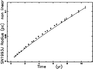
Fig. 1 : Theoretical radius as obtained by the solution of the equation (9) (full line), data and merit function , $\chi^{2}$ , as in Table 1. The astronomical data of SN  1993J are represented through empty stars.

Table 1 : Numerical value of the parameters of the fits for SN  1993J and $\chi^{2}$. $N$ represents the number of free parameters. PL stands for power law and NLR for non linear radius.

$\displaystyle\hskip 0.0pt{\begin{array}[]{cccc}\hline\cr\hline\cr\vskip 6.0pt\cr keyword&N&values&\chi^{2}\\ \vskip 6.0pt\cr\hline\cr\vskip 6.0pt\cr PL&2&\alpha_{obs}=0.82;r_{obs}=0.015~{}pc&6364\\ \vskip 6.0pt\cr\hline\cr NLR&4&p=18.8;&623.5\\ {}\hfil&{}\hfil&r_{0}=2.25\,10^{-8}~{}pc;&{}\hfil\\ \vskip 6.0pt\cr{}\hfil&{}\hfil&t_{0}=4.98\,0^{-8}~{}yr;&{}\hfil\\ {}\hfil&{}\hfil&v_{0}=100000\frac{km}{s}&{}\hfil\\ \vskip 6.0pt\cr\hline\cr\hline\cr\end{array}}$

The quality of the fits is measured by the merit function $\chi^{2}$

$$\chi^{2}=\sum_{j}\frac{(R_{th}-R_{obs})^{2}}{\sigma_{obs}^{2}}\quad,$$ (16)

where $R_{th}$, $R_{obs}$ and $\sigma_{obs}$ are the theoretical radius, the observed radius and the observed uncertainty respectively.

The conservation of classical momentum here adopted does not take into account the momentum carried away by photons or in other words the radiative losses are included in the NCD exponent.

4 Asymmetrical law of motion with NCD

Given the Cartesian coordinate system $(x,y,z)$ , the plane $z=0$ will be called equatorial plane and in polar coordinates $z=R\sin(\theta)$, where $\theta$ is the polar angle and $R$ the distance from the origin . The presence of a non homogeneous medium in which the expansion takes place is here modeled assuming an exponential behavior for the number of particles of the type

$$n(z)=n_{0}\exp{-\frac{z}{h}}\quad=n_{0}\exp{-\frac{R\times\sin(\theta)}{h}}\quad,$$ (17)

where $R$ is the radius of the shell, $n_{0}$ is the number of particles at $R=R_{0}$ and $h$ the scale. The 3D expansion will be characterized by the following properties

• Dependence of the momentary radius of the shell on the polar angle $\theta$ that has a range $[-90^{\circ}\leftrightarrow+90^{\circ}]$.

• Independence of the momentary radius of the shell from $\phi$ , the azimuthal angle in the x-y plane, that has a range $[0^{\circ}\leftrightarrow 360^{\circ}]$.

The mass swept, $M$, along the solid angle $\Delta\;\Omega$, between 0 and $R$ is

$$M(R)=\frac{\Delta\;\Omega}{3}m_{H}n_{0}I_{m}(R)+\frac{4}{3}\pi R_{0}^{3}n_{0}m_{H}\quad,$$ (18)

where

$$I_{m}(R)=\int_{R_{0}}^{R}r^{2}\exp{-\frac{r\sin(\theta)}{h}}dr\quad,$$ (19)

where $R_{0}$ is the initial radius and $m_{H}$ the mass of the hydrogen. The integral is

$$I_{m}(R)=$$

$$\frac{h\left(2{h}^{2}+2R_{0}h\sin\left(\theta\right)+{R_{0}}^{2}\left(\sin\left(\theta\right)\right)^{2}\right){{\rm e}^{-{\frac{R_{0}\sin\left(\theta\right)}{h}}}}}{\left(\sin\left(\theta\right)\right)^{3}}$$

$$-\frac{h\left(2{h}^{2}+2Rh\sin\left(\theta\right)+{R}^{2}\left(\sin\left(\theta\right)\right)^{2}\right){{\rm e}^{-{\frac{R\sin\left(\theta\right)}{h}}}}}{\left(\sin\left(\theta\right)\right)^{3}}\quad.$$ (20)

The conservation of the momentum gives

$$(M(R))^{\frac{1}{p}}\dot{R}=(M(R_{0}))^{\frac{1}{p}}\dot{R_{0}}\quad,$$ (21)

where $\dot{R}$ is the velocity at $R$ and $\dot{R_{0}}$ is the initial velocity at $R=R_{0}$ where $p$ is the NCD parameter. This means that only a fraction of the total mass enclosed in the volume of the expansion accumulates in a thin shell just after the shock front. According to the previous expression the velocity is

$$V(R)={{\it R_{0}}}^{3{p}^{-1}}{\it V_{0}}((-2{h}^{3}{{\rm e}^{-{\frac{R\sin(\theta)}{h}}}}$$

$$-2{h}^{2}{{\rm e}^{-{\frac{R\sin(\theta)}{h}}}}R\sin(\theta)$$

$$-h{{\rm e}^{-{\frac{R\sin(\theta)}{h}}}}{R}^{2}(\sin(\theta))^{2}+2{h}^{3}{{\rm e}^{-{\frac{{\it R_{0}}\sin(\theta)}{h}}}}$$

$$+2{h}^{2}{{\rm e}^{-{\frac{{\it R_{0}}\sin(\theta)}{h}}}}{\it R_{0}}\sin(\theta)+h{{\rm e}^{-{\frac{{\it R_{0}}\sin(\theta)}{h}}}}{{\it R_{0}}}^{2}(\sin(\theta))^{2}$$

$$+{{\it R_{0}}}^{3}(\sin(\theta))^{3})(\sin(\theta))^{-3})^{-{p}^{-1}}\quad.$$ (22)

In this differential equation of the first order in $R$ the variable can be separated and the integration term by term gives

$$\int_{R_{0}}^{R}(M(r))^{1/p}dr=(M(R_{0}))^{1/p}\dot{R_{0}}\times(t-t_{0})\quad,$$ (23)

where $t$ is the time and $t_{0}$ the time at $R_{0}$. The resulting non linear equation ${\mathcal{F}}_{NL}$ expressed in astrophysical units is

$${\mathcal{F}}_{NL}=\int_{R_{0,pc}}^{R_{pc}}{3}^{-{p}^{-1}}((-2{h_{pc}}^{3}{{\rm e}^{-{\frac{{r_{pc}}\sin(\theta)}{h_{pc}}}}}$$

$$-2{h_{pc}}^{2}{{\rm e}^{-{\frac{{r_{pc}}\sin(\theta)}{h_{pc}}}}}{r_{pc}}\sin(\theta)$$

$$-h{{\rm e}^{-{\frac{{r_{pc}}\sin(\theta)}{h_{pc}}}}}{{r_{pc}}}^{2}(\sin(\theta))^{2}$$

$$+2{h_{pc}}^{3}{{\rm e}^{-{\frac{{\it{R_{0,pc}}}\sin(\theta)}{h_{pc}}}}}+2{h_{pc}}^{2}{{\rm e}^{-{\frac{{\it{R_{0,pc}}}\sin(\theta)}{h_{pc}}}}}{\it{R_{0,pc}}}\sin(\theta)$$

$$+h{{\rm e}^{-{\frac{{\it{R_{0,pc}}}\sin(\theta)}{h_{pc}}}}}{{\it{R_{0,pc}}}}^{2}(\sin(\theta))^{2}$$

$$+{{\it{R_{0,pc}}}}^{3}(\sin(\theta))^{3})(\sin(\theta))^{-3})^{{p}^{-1}}dr$$

$$-1.0210^{-5}{3}^{-{p}^{-1}}{{\it R_{0,pc}}}^{3{p}^{-1}}{\it\dot{R}_{0,kms}}(t_{1}-{\it t_{0,1}})=0$$ (24)

where $t_{1}$ and $t_{0,1}$ are $t$ and $t_{0}$ expressed in yr units, $r_{pc}$ and $R_{0,pc}$ are $R$ and $R_{0}$ expressed in $pc$, $\dot{R}_{0,kms}$ is $\dot{R}_{0}$ expressed in $\frac{km}{s}$, $\theta$ is expressed in radians and $h_{pc}$ is the the scale , $h$ , expressed in $pc$. It is not possible to find $R_{pc}$ analytically and a numerical method should be implemented. In our case in order to find the root of ${\mathcal{F}}_{NL}$, the FORTRAN SUBROUTINE ZRIDDR from Press et al. (1992) has been used.

5 Applications of the law of motion

From a practical point of view, $\epsilon$ , the percentage of reliability of our code is introduced,

$$\epsilon=(1-\frac{|(R_{\mathrm{pc,obs}}-R_{pc,\mathrm{num}})|}{R_{pc,\mathrm{obs}}})\cdot 100,$$ (25)

where $R_{pc,\mathrm{obs}}$ is the radius as given by the astronomical observations in parsec , and $R_{pc,\mathrm{num}}$ the radius obtained from our simulation in parsec.

5.1 Results on the strongly asymmetric SN  1987A 

The first target is to simulate the torus only of SN  1987A  (our equatorial plane) and this operation allows to calibrate our code ; Table 2 reports the input data, Figs. 2 and 3 the behavior of radius and velocity respectively as function of the time. Due to the complexity of the 3D structure we report the reliability of the simulation only in the equatorial plane (torus only) which is $\epsilon=91.4\%$ for the radii and $\epsilon=38.3\%$ for the velocity.

Table 2 : Numerical value of the parameters of the simulation for SN  1987A 

$\displaystyle\hskip 0.0pt{\begin{array}[]{lc}\hline\cr\hline\cr R_{0,pc}&0.014\\ \dot{R}_{0,kms}&26000\\ p&4\\ t_{0,1}&0.0218\\ t_{1}&21.86\\ \vskip 6.0pt\cr\hline\cr\hline\cr\end{array}}$

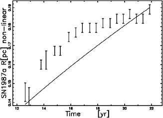
Fig. 2 : Radius as a function of time for an exponentially varying medium (full line) when $\theta=0.001$ (equatorial plane) and astronomical data of torus only as extracted from Table 2 in Racusin et al. (2009). Physical parameters as in Table 2.

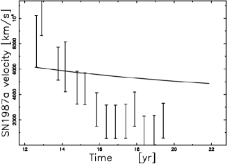
Fig. 3 : Velocity as a function of the time for an exponentially varying medium (full line) when $\theta=0.001$ (equatorial plane) and astronomical velocities as deduced from Table 2 in Racusin et al. (2009). Physical parameters as in Table 2.

After this calibration on the equatorial plane we continue identifying the lobes of SN  1987A  as bipolar SNR as seen from a given point of view. The complex 3D behavior of the advancing SNR is reported in Fig. 4 and Fig. 5 reports the asymmetric expansion in a section crossing the center. In order to better visualize the asymmetries Figs. 6 and 7 report the radius and the velocity respectively as a function of the position angle $\theta$. The combined effect of spatial asymmetry and field of velocity are reported in Fig. 8.

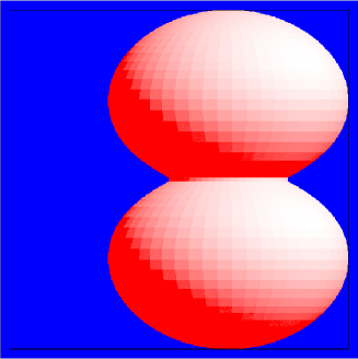
Fig. 4 : Continuous three-dimensional surface of SN  1987A  : the three Eulerian angles characterizing the point of view are $\Phi$=90 ^∘, $\Theta$=90 ^∘ and $\Psi$=90 ^∘. Physical parameters as in Table 2.

Fig. 5 : Section of SN  1987A  in the x-z plane. The horizontal and vertical axis are in $pc$. Physical parameters as in Table 2.

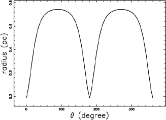
Fig. 6 : Radius in $pc$ of SN  1987A  as a function of the position angle in degrees. Physical parameters as in Table 2.

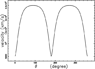
Fig. 7 : Velocity in $\frac{km}{s}$ of SN  1987A  as a function of the position angle in degrees. Physical parameters as in Table 2.

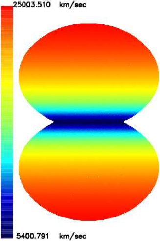
Fig. 8 : Map of the expansion velocity in $\frac{km}{s}$ relative to the simulation of SN  1987A  when 300000 random points are selected on the surface. Physical parameters as in Table 7.

An explanation for the lack of velocity in the equatorial region of SN  1987A  can be drawn from a careful analysis of Fig. 9 which displays the swept mass as a function of the latitude. The ratio between maximum swept mass in the polar direction and minimum swept mass in the equatorial plane is $\approx$ 5.5 . On applying the momentum conservation the velocity in the equatorial plane is 5.5 times smaller in respect to the polar direction where the velocity is maximum. This numerical evaluation gives a simple explanation for the asymmetry of SN  1993J : a smaller mass being swept means a greater velocity of the advancing radius of the nebula.

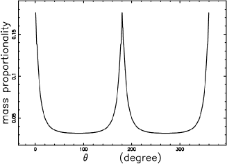
Fig. 9 : Swept mass of SN  1987A  as a function of the position angle in degrees in arbitrary units. Physical parameters as in Table 2.

5.2 Results on the weakly asymmetric SN  1006 

The input data of the simulation are reported in Table 3 ; the reliability is $\epsilon=89\%$ for the radii in the equatorial direction and $\epsilon=89\%$ for the velocity in the equatorial direction.

Table 3 : Numerical value of the parameters of the simulation for SN  1006 .

$\displaystyle\hskip 0.0pt{\begin{array}[]{lc}\hline\cr\hline\cr R_{0,pc}&0.09\\ \dot{R}_{0,kms}&8500\\ p&30\\ t_{0,1}&10\\ t_{1}&1000\\ \vskip 6.0pt\cr\hline\cr\hline\cr\end{array}}$

The weakly asymmetric 3D shape of SN  1006  is reported in Fig. 10.

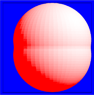
Fig. 10 : Continuous three-dimensional surface of the SN  1006  : the three Eulerian angles characterizing the point of view are $\Phi$=90 ^∘, $\Theta$=90 ^∘ and $\Psi$=90 ^∘. Physical parameters as in Table 2.

The velocity as function of the position angle is plotted in Fig. 11 and a comparison should be done with Fig. 4 in Katsuda et al. (2009) where the proper motion as function of the azimuth angle was reported.

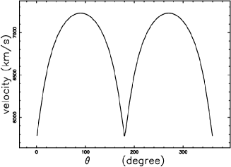
Fig. 11 : Velocity in $\frac{km}{s}$ of SN  1006  as a function of the position angle in degrees. Physical parameters as in Table 2.

Our model for SN  1006  predicts a minimum velocity in the equatorial plane of 5785 $km/s$ and a maximum velocity of 7229 $km/s$ in the polar direction. A recent observation of SN  1006  quotes a minimum velocity of 5500 $km/s$ and a maximum velocity of 14500 $km/s$ assuming a distance of = 3.4 kpc The swept mass in the thin layer versus the position angle is displayed in Fig. 12.

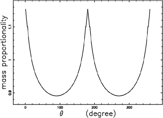
Fig. 12 : Swept mass of SN  1006  as a function of the position angle in degrees in arbitrary units. Physical parameters as in Table 3.

5.3 Comparison with the stellar wind

A comparison can be done with the expansion speed of the outer $H_{2}$ shell of $\eta$-Carinae which has been fitted with the following latitude dependent velocity

$$v=\frac{{\it v_{1}}\,\left({\it v_{2}}+{{\rm e}^{2\,{\it\lambda}\,\cos\left(2\,\Theta\right)}}{\it v_{1}}\right)}{{\it v_{1}}\,\left(1+{{\rm e}^{2\,{\it\lambda}\,\cos\left(2\,\Theta\right)}}\right)}\quad,$$ (26)

where the parameter $\lambda$ controls the shape of the Homunculus, $\Theta$ is the polar angle; $v_{1}$ and $v_{2}$ are the velocities in the polar and equatorial direction, see González et al. (2010). Fig. 13 the data of our simulation as well the wind-type profile of velocity.

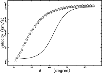
Fig. 13 : Expansion velocity versus latitude of SN  1987A  ( open stars) and fit as given by formula (26) (full line). The fitting parameters are : $\lambda$=1.9, $v_{1}=2503.6\,km/s$ and $v_{2}=5401\,km/s$.

6 Radiative transfer equation

The transfer equation in the presence of emission only , see for example Rybicki and Lightman (1991) or Hjellming, R. M. (1988), is

$$\frac{dI_{\nu}}{ds}=-k_{\nu}\zeta I_{\nu}+j_{\nu}\zeta\quad,$$ (27)

where $I_{\nu}$ is the specific intensity , $s$ is the line of sight , $j_{\nu}$ the emission coefficient, $k_{\nu}$ a mass absorption coefficient, $\zeta$ the mass density at position $s$ and the index $\nu$ denotes the interested frequency of emission. The solution to equation (27) is

$$I_{\nu}(\tau_{\nu})=\frac{j_{\nu}}{k_{\nu}}(1-e^{-\tau_{\nu}(s)})\quad,$$ (28)

where $\tau_{\nu}$ is the optical depth at frequency $\nu$

$$d\tau_{\nu}=k_{\nu}\zeta ds\quad.$$ (29)

We now continue analyzing the case of an optically thin layer in which $\tau_{\nu}$ is very small ( or $k_{\nu}$ very small ) and the density $\zeta$ is substituted with our number density $C(s)$ of particles. One case is taken into account : the emissivity is proportional to the number density.

$$j_{\nu}\zeta=KC(s)\quad,$$ (30)

where $K$ is a constant function. This can be the case of synchrotron radiation in presence of a isotropic distribution of electrons with a power law distribution in energy, $N(E)$,

$$N(E)dE=K_{s}E^{-\gamma_{f}}\quad,$$ (31)

where $K_{s}$ is a constant. In this case the emissivity is

$$j_{\nu}\rho\approx 0.933\times 10^{-23}\alpha(\gamma_{f})K_{s}H_{\perp}^{\frac{\gamma_{f}+1}{2}}\times$$

$$\bigl{(}\frac{6.26\times 10^{18}}{\nu}\bigr{)}^{\frac{\gamma_{f}-1}{2}}\frac{erg}{scm^{3}Hzrad^{2}},$$ (32)

where $\nu$ is the frequency and $\alpha(\gamma_{f})$ is a slowly varying function of $\gamma_{f}$ which is of the order of unity and is given by

$$\alpha(\gamma_{f})=$$

$$2^{(\gamma_{f}-3)/2}\frac{\gamma_{f}+7/3}{\gamma_{f}+1}\Gamma\bigl{(}\frac{3\gamma_{f}-1}{12}\bigr{)}\Gamma\bigl{(}\frac{3\gamma_{f}+7}{12}\bigr{)}\quad,$$ (33)

for $\gamma_{f}\geq\frac{1}{2}$, see formula (1.175 ) in Lang (1999). The source of synchrotron luminosity is assumed here to be the flux of kinetic energy, $L_{m}$,

$$L_{m}=\frac{1}{2}\rho AV^{3}\quad,$$ (34)

where $A$ is the considered area, see formula (A28) in de Young (2002). In our case $A=4\pi R^{2}$, which means

$$L_{m}=\frac{1}{2}\rho 4\pi R^{2}V^{3}\quad,$$ (35)

where $R$ is the instantaneous radius of the SNR and $\rho$ is the density in the advancing layer in which the synchrotron emission takes place. The total observed luminosity can be expressed as

$$L_{tot}=\epsilon L_{m}\quad,$$ (36)

where $\epsilon$ is a constant of conversion from the mechanical luminosity to the total observed luminosity in synchrotron emission. The fraction of the total luminosity deposited in a given band $f_{b}$ is

$$f_{b}=\frac{{{\it\nu_{b,min}}}^{-\gamma_{f}+1}-{{\it\nu_{b,max}}}^{-\gamma_{f}+1}}{{{\it\nu_{min}}}^{-\gamma_{f}+1}-{{\it\nu_{max}}}^{-\gamma_{f}+1}}\quad,$$ (37)

where $\nu_{b,min}$ and $\nu_{b,max}$ are the minimum and maximum frequency of the given band.

7 Image

An simulated image of an astrophysical object is composed by combining the intensities which characterize different points. For an optically thin medium the transfer equation provides the emissivity to be multiplied with the distance on the line of sight , $l$. This length in astrophysical diffuse objects depends on the orientation of the observer. A thermal and a non thermal model are reviewed in the spherical case. In the the aspherical case a non thermal model is presented.

7.1 Spherical Image

A first thermal model for the image is characterized by a constant temperature in the internal region of the advancing sphere. We therefore assume that the number density $C$ is constant in a sphere of radius $a$ and then falls to 0. The length of sight , when the observer is situated at the infinity of the $x$-axis , is the locus parallel to the $x$-axis which crosses the position $y$ in a Cartesian $x-y$ plane and terminates at the external circle of radius $a$, see Zaninetti (2009). The locus length is

$$l_{ab}=2\times(\sqrt{a^{2}-y^{2}})\quad;0\leq y<a\quad.$$ (38)

The number density $C_{m}$ is constant in the sphere of radius $a$ and therefore the intensity of radiation is

$$I_{0a}=C_{m}\times 2\times(\sqrt{a^{2}-y^{2}})\quad;0\leq y<a\quad.$$ (39)

The comparison of observed data of SN  1993J and the theoretical thermal intensity is reported in Fig. 14.

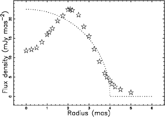
Fig. 14 : Cut of the thermal intensity ${\it I}$ of the rim model ( equation (39)) through the center (dotted line) of SN  1993J and real data (empty stars) when $b=0.07$pc. The observed data as day 1889 after the explosion have been extracted by the author from Fig. 3 of Marcaide et al. (2009).

A second non thermal model for the image is characterized by emission in a thin layer around the advancing sphere. We therefore assume that the number density $C$ is constant and in particular rises from 0 at $r=a$ to a maximum value $C_{m}$ , remains constant up to $r=b$ and then falls again to 0. The length of sight , when the observer is situated at the infinity of the $x$-axis , is the locus parallel to the $x$-axis which crosses the position $y$ in a Cartesian $x-y$ plane and terminates at the external circle of radius $b$, see Zaninetti (2009). The locus length is

$$l_{0a}=2\times(\sqrt{b^{2}-y^{2}}-\sqrt{a^{2}-y^{2}})\quad;0\leq y<a$$

$$l_{ab}=2\times(\sqrt{b^{2}-y^{2}})\quad;a\leq y<b\quad.$$ (40)

The number density $C_{m}$ is constant between two spheres of radius $a$ and $b$ and therefore the intensity of radiation is

$$I_{0a}=C_{m}\times 2\times(\sqrt{b^{2}-y^{2}}-\sqrt{a^{2}-y^{2}})\quad;0\leq y<a$$

$$I_{ab}=C_{m}\times 2\times(\sqrt{b^{2}-y^{2}})\quad;a\leq y<b\quad.$$ (41)

The comparison of observed data of SN  1993J and the theoretical non thermal intensity is displayed in Fig.  15.

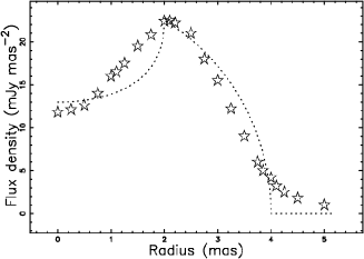
Fig. 15 : Cut of the non thermal intensity ${\it I}$ of the rim model ( equation (41)) through the center (dotted line) of SN  1993J and real data (empty stars). The parameters are $a=0.0035$ pc and $b=0.07$pc. Observed data as day 1889 after the explosion have been extracted by the author from Fig. 3 of Marcaide et al. (2009).

The main result of this Section is that the intensity of the thermal model which has the maximum of the intensity at the center of SNR does not match with the observed profiles. The observed profiles in the intensity have the maximum value at the rim as predicted by the non thermal model.

7.2 Aspherical Image

The numerical algorithm which allows us to build a complex image is now outlined.

• An empty (value=0) memory grid ${\mathcal{M}}(i,j,k)$ which contains $NDIM^{3}$ pixels is considered

• We first generate an internal 3D surface by rotating the ideal image $180^{\circ}$ around the polar direction and a second external surface at a fixed distance $\Delta R$ from the first surface. As an example, we fixed $\Delta R$ = $0.03R_{max}$, where $R_{max}$ is the maximum radius of expansion. The points on the memory grid which lie between the internal and external surfaces are memorized on ${\mathcal{M}}(i,j,k)$ with a variable integer number according to formula (35) and density $\rho$ proportional to the swept mass, see Fig. 9.

• Each point of ${\mathcal{M}}(i,j,k)$ has spatial coordinates $x,y,z$ which can be represented by the following $1\times 3$ matrix, $A$,

  $$A=\left[\begin{array}[]{c}x\\ \vskip 12.5pt\cr y\\ \vskip 12.5pt\cr{\it z}\end{array}\right]\quad.$$ (42)

  The orientation of the object is characterized by the Euler angles $(\Phi,\Theta,\Psi)$ and therefore by a total $3\times 3$ rotation matrix, $E$, see Goldstein, Poole, and Safko (2002). The matrix point is represented by the following $1\times 3$ matrix, $B$,

  $$B=E\cdot A\quad.$$ (43)

• The intensity map is obtained by summing the points of the rotated images along a particular direction.

• The effect of the insertion of a threshold intensity , $I_{tr}$, given by the observational techniques , is now analyzed. The threshold intensity can be parametrized to $I_{max}$, the maximum value of intensity characterizing the map.

7.3 The image of the strongly asymmetric SN  1987A 

An ideal image of SN  1987A  having the polar axis aligned with the z-direction which means polar axis along the z-direction, is shown in Fig. 16. A model for a realistically rotated SN  1987A  is shown in Fig. 17.

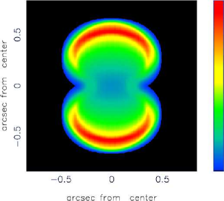
Fig. 16 : Map of the theoretical intensity of SN  1987A  in the presence of an exponentially varying medium. Physical parameters as in Table 2. The three Euler angles characterizing the orientation are $\Phi$=180^∘, $\Theta$=90 ^∘ and $\Psi$=0 ^∘. This combination of Euler angles corresponds to the rotated image with the polar axis along the z-axis.

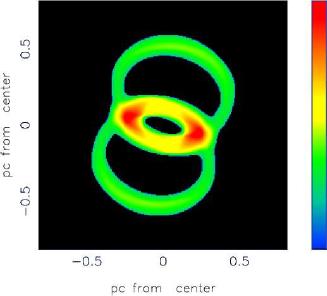
Fig. 17 : Model map of SN  1987A  rotated in accordance with the observations, for an exponentially varying medium. Physical parameters as in Table 2. The three Euler angles characterizing the orientation of the observer are $\Phi$=105^∘, $\Theta$=55 ^∘ and $\Psi$=-165 ^∘. This combination of Euler angles corresponds to the observed image. In this map $I_{tr}=I_{max}/4$

The three rings of SN  1987A  are now simulated in our Fig. 17 and a comparison should be done with Fig. 1 in Tziamtzis et al. (2011) in which the HST/ACS image (filter F658N) of the triple ring system of SN  1987A  was reported.

7.4 The image of the weakly asymmetric SN  1006 

The image of SN  1006  is visible in different bands such as radio, see Reynolds and Gilmore (1993); Reynoso (2007), optical , see Long (2007) and X-ray , see Dyer, Reynolds, and Borkowski (2004); Katsuda et al. (2010). The 2D map in intensity of SN  1006  is visible in Fig. 18.

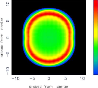
Fig. 18 : Non rotated map of SN  1006  for an exponentially varying medium. Physical parameters as in Table 3.

The intensity along the equatorial and polar direction of our image is reported in Fig. 19; a comparison should be done with Fig. 4 in Dyer, Reynolds, and Borkowski (2004).

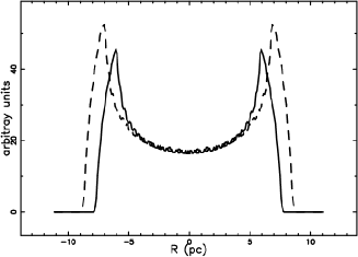
Fig. 19 : Two cut along perpendicular lines of I for the non rotated image of SNR SN  1006 .

The projected flux as a function of the position angle is another interesting quantity to plot , see Fig. 20 and a comparison should be done with Fig. 5 top right in Rothenflug et al. (2004).

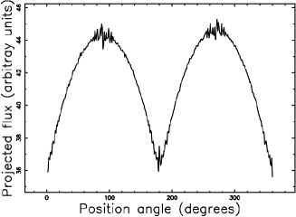
Fig. 20 : Intensity as function of the position angle in degrees for SNR SN  1006 .

After the previous graphs is more simple to present a characteristic feature as the ”jet appearance” visible in some maps , see our Fig. 21; a comparison should be done with the X-map at 6.33-6.53 kev band visible in Fig. 3b by Yamaguchi et al. (2008).

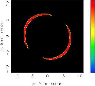
Fig. 21 : Model map of SN  1006  rotated in accordance with the X observations, for an exponentially varying medium. Physical parameters as in Table 3. The three Euler angles characterizing the orientation of the observer are $\Phi$=90 ^∘, $\Theta$=-55 ^∘ and $\Psi$=-180 ^∘. This combination of Euler angles corresponds to the observed image. In this map $I_{tr}=I_{max}/1.1$

8 Conclusions

Law of motion

We have deduced a new law of motion in spherical symmetry ( constant density) for an advancing shell assuming that only a fraction of the mass which resides in the surrounding medium is accumulated in the advancing layer, see equation (9). The presence of an exponential law for the density transforms the spherical symmetry in axial symmetry and allows the appearance of the so called ”bipolar motion”, see the nonlinear astrophysical equation (24).

Images

The emissivity in the advancing layer is assumed to be proportional to the flux of kinetic energy, see equation (34) where the density is assumed to be proportional to the swept material. This assumption allows to simulate particular effects such as the triple ring system of SN  1987A , see Fig. 17. Another curious effect is the ”jet appearance” visible in the weakly symmetric SN  1006 , see Fig. 21. The jet/counter jet effect plays a relevant role in the actual research , see discussion in Section 5.2 in Fesen et al. (2006) where the jet appearance is tentatively explained by the neutrino heating , see Walder et al. (2005) or by the MHD jet , see Takiwaki et al. (2004). Here conversely we explain the appearance of the jet by the addition of three effects :

• An asymmetric law of expansion due to a gradient in density in respect to the equatorial plane which produces an asymmetry in velocity .

• The direct conversion of the flux of kinetic energy into radiation.

• The image of the SNR as the composition of integrals along the line of sight.

According to the previous three ingredients the neutrino heating mechanism is not necessary. The Magneto Hydrodynamic (MHD) approach is supposed to act in a hidden way on scales smaller than than the thickness of the advancing layer in order to accelerate the electrons to relativistic energies. A careful calibration of the various involved parameters can be done when cuts in intensity are available.

References

- Bamba et al. (2003) Bamba, A., Yamazaki, R., Ueno, M., Koyama, K.: ApJ 589, 827 (2003)
- Cantó, Raga, and Adame (2006) Cantó, J., Raga, A.C., Adame, L.: MNRAS 369, 860 (2006)
- de Young (2002) de Young, D.S.: The physics of extragalactic radio sources. University of Chicago Press, Chicago (2002)
- Dyer, Reynolds, and Borkowski (2004) Dyer, K.K., Reynolds, S.P., Borkowski, K.J.: ApJ 600, 752 (2004)
- Dyson (1983) Dyson, J.E.: A&A 124, 77 (1983)
- Dyson, J. E. and Williams, D. A. (1997) Dyson, J. E. and Williams, D. A.: The physics of the interstellar medium. Institute of Physics Publishing, Bristol (1997)
- Ellison et al. (1994) Ellison, D.C., Reynolds, S.P., Borkowski, K., Chevalier, R., Cox, D.P., Dickel, J.R., Pisarski, R., Raymond, J., Spangler, S.R., Volk, H.J., Wefel, J.P.: PASP 106, 780 (1994)
- Eriksen et al. (2009) Eriksen, K.A., Arnett, D., McCarthy, D.W., Young, P.: ApJ 697, 29 (2009)
- Fesen et al. (2006) Fesen, R.A., Hammell, M.C., Morse, J., Chevalier, R.A., Borkowski, K.J., Dopita, M.A., Gerardy, C.L., Lawrence, S.S., Raymond, J.C., van den Bergh, S.: ApJ 645, 283 (2006). doi:10.1086/504254
- Goldstein, Poole, and Safko (2002) Goldstein, H., Poole, C., Safko, J.: Classical mechanics. Addison-Wesley, San Francisco (2002)
- González et al. (2010) González, R.F., Villa, A.M., Gómez, G.C., de Gouveia Dal Pino, E.M., Raga, A.C., Cantó, J., Velázquez, P.F., de La Fuente, E.: MNRAS 402, 1141 (2010)
- Hjellming, R. M. (1988) Hjellming, R. M.: Radio stars IN Galactic and Extragalactic Radio Astronomy . Springer, New York (1988)
- Katsuda et al. (2009) Katsuda, S., Petre, R., Long, K.S., Reynolds, S.P., Winkler, P.F., Mori, K., Tsunemi, H.: ApJ 692, 105 (2009)
- Katsuda et al. (2010) Katsuda, S., Petre, R., Mori, K., Reynolds, S.P., Long, K.S., Winkler, P.F., Tsunemi, H.: ApJ 723, 383 (2010)
- Lang (1999) Lang, K.R.: Astrophysical formulae. (Third Edition). Springer, New York (1999)
- Long (2007) Long, K.S.: Highlights of Astronomy 14, 306 (2007)
- Marcaide et al. (2009) Marcaide, J.M., Martí-Vidal, I., Alberdi, A., Pérez-Torres, M.A.: A&A 505, 927 (2009)
- McCray and Layzer (1987) McCray, A. R. In: Dalgarno, Layzer, D. (eds.): Spectroscopy of astrophysical plasmas. Cambridge University Press, Cambridge (1987)
- McKee (1987) McKee, C.F.: In: Dalgarno, A., Layzer, D. (eds.) Spectroscopy of Astrophysical Plasmas, p. 226 (1987)
- Mitchell et al. (2002) Mitchell, R.C., Baron, E., Branch, D., Hauschildt, P.H., Nugent, P.E., Lundqvist, P., Blinnikov, S., Pun, C.S.J.: ApJ 574, 293 (2002)
- Panagia (2005) Panagia, N.: In: Marcaide, J.M., Weiler, K.W. (eds.) IAU Colloq. 192: Cosmic Explosions, On the 10th Anniversary of SN1993J, p. 585 (2005)
- Petruk and Beshlei (2007) Petruk, O., Beshlei, V.: Kinematics and Physics of Celestial Bodies 23, 16 (2007)
- Press et al. (1992) Press, W.H., Teukolsky, S.A., Vetterling, W.T., Flannery, B.P.: Numerical Recipes in FORTRAN. The Art of Scientific Computing. Cambridge University Press, Cambridge (1992)
- Racusin et al. (2009) Racusin, J.L., Park, S., Zhekov, S., Burrows, D.N., Garmire, G.P., McCray, R.: ApJ 703, 1752 (2009)
- Reynolds and Gilmore (1986) Reynolds, S.P., Gilmore, D.M.: AJ 92, 1138 (1986)
- Reynolds and Gilmore (1993) Reynolds, S.P., Gilmore, D.M.: AJ 106, 272 (1993)
- Reynoso (2007) Reynoso, E.M.: Highlights of Astronomy 14, 305 (2007)
- Rothenflug et al. (2004) Rothenflug, R., Ballet, J., Dubner, G., Giacani, E., Decourchelle, A., Ferrando, P.: A&A 425, 121 (2004)
- Rybicki and Lightman (1991) Rybicki, G., Lightman, A.: Radiative processes in astrophysics. Wiley-Interscience, New-York (1991)
- Sedov (1959) Sedov, L.I.: Similarity and Dimensional Methods in Mechanics. Academic Press, New York (1959)
- Strom (1988) Strom, R.G.: MNRAS 230, 331 (1988)
- Takiwaki et al. (2004) Takiwaki, T., Kotake, K., Nagataki, S., Sato, K.: ApJ 616, 1086 (2004). doi:10.1086/424993
- Taylor (1950) Taylor, G.: Royal Society of London Proceedings Series A 201, 159 (1950)
- Tziamtzis et al. (2011) Tziamtzis, A., Lundqvist, P., Gröningsson, P., Nasoudi-Shoar, S.: A&A 527, 35 (2011)
- Vink (2005) Vink, J.: In: R. Smith (ed.) X-ray Diagnostics of Astrophysical Plasmas: Theory, Experiment, and Observation. American Institute of Physics Conference Series vol. 774, p. 241 (2005)
- Walder et al. (2005) Walder, R., Burrows, A., Ott, C.D., Livne, E., Lichtenstadt, I., Jarrah, M.: ApJ 626, 317 (2005). doi:10.1086/429816
- Yamaguchi et al. (2008) Yamaguchi, H., Koyama, K., Katsuda, S., Nakajima, H., Hughes, J.P., Bamba, A., Hiraga, J.S., Mori, K., Ozaki, M., Tsuru, T.G.: PASJ 60, 141 (2008)
- Zaninetti (2004) Zaninetti, L.: PASJ 56, 1067 (2004)
- Zaninetti (2009) Zaninetti, L.: MNRAS 395, 667 (2009)
- Zaninetti (2011) Zaninetti, L.: Astrophysics and Space Science 333, 99 (2011)