Entanglement Creation in Low-Energy Scattering

Abstract

We study the entanglement creation in the low-energy scattering of two particles in three dimensions, for a general class of interaction potentials that are not required to be spherically symmetric. The incoming asymptotic state, before the collision, is a product of two normalized Gaussian states. After the scattering the particles are entangled. We take as a measure of the entanglement the purity of one of them. We provide a rigorous explicit computation, with error bound, of the leading order of the purity at low-energy. The entanglement depends strongly in the difference of the masses. It takes its minimum when the masses are equal, and it increases rapidly with the difference of the masses. It is quite remarkable that the anisotropy of the potential gives no contribution to the leading order of the purity, on spite of the fact that entanglement is a second order effect.

1 Introduction

In this paper we study how entanglement is created in a scattering process. This topic has intrinsic interest. As is well known, scattering is a basic dynamical process that is essential across all areas of physics. Entanglement is a central notion of modern quantum theory, in particular, it is the fundamental resource for quantum information theory and quantum computation. It is a measure for quantum correlations between subsystems. In the case of bipartite systems in pure states, entanglement is a measure of how far away from being a product state a pure state of the bipartite system is. Product states are called disentangled. It is now well understood that entanglement in a pure bipartite quantum state is equivalent to the degree of mixedness of each subsystem. See, for example [1], [2], [3]. Moreover, the study of entanglement creation in scattering is interesting for a many other reasons. For example, for the implementation of quantum information processes in physical systems where scattering is central to the dynamics, like ultracold atoms and solid state devices. Moreover, the study of entanglement in the scattering of particles requires quantum information theory with continuous variables and mixed continuous-discrete variables. See [3] for a review of this topic. As scattering interactions are fundamental at all scales, and as there is a large variety of scattering systems, it is possible that scattering will provide a new perspective to quantum information theory. Finally, entanglement creation is important to the theory of scattering itself, because it poses new problems that can shed some new light and new points of view in the study of scattering processes.

Actually, from the conceptual point of view scattering is perhaps the simplest way to entangle two particles. Before the scattering, in the incoming state, the two particles are in a pure product state where they are uncorrelated. As they approach each other they become entangled by sharing quantum information between them. After the scattering, when they are far apart from each other, they remain entangled in the outgoing asymptotic state, that is not a product state anymore.

We take as measure of entanglement of a pure state the purity of one of the particles, that is to say, the trace of the square of the reduced density matrix of one of the particles, that is obtained by taking the trace on the other particle of the density matrix of the pure state. The purity of a product state is one.

We consider two spinless particles in three dimensions with the interaction given by a general potential that is not required to be spherically symmetric. Initially the particles are in an incoming asymptotic state that is a product of two Gaussian states. After the scattering the particles are in an outgoing asymptotic state that, as mentioned above, is not a product state and our problem is to determine the loss of purity of one of the particles, due to the entanglement with the other that is produced by the scattering process.

The Hilbert space of states for the two particles in the configuration representation is $\mathcal{H}:=L^{2}({\mathbb{R}}^{6})$. The Schrödinger equation is

$$i\hbar\frac{\partial}{\partial t}\varphi(\mathbf{x}_{1},\mathbf{x}_{2})=H\varphi(\mathbf{x}_{1}.\mathbf{x}_{2}),$$ (1.1)

where the Hamiltonian is given by

$$H=H_{0}+V(\mathbf{x}_{1}-\mathbf{x}_{2}),$$ (1.2)

with $H_{0}$ is the free Hamiltonian,

$$H_{0}:=-\frac{\hbar^{2}}{2m_{1}}\Delta_{1}-\frac{\hbar^{2}}{2m_{2}}\Delta_{2},$$ (1.3)

where $\hbar$ is Planck’s constant, $m_{j},j=1,2$, are, respectively, the mass of particle one and two, and $\Delta_{j}$, the Laplacian in the coordinates $\mathbf{x}_{j},j=1,2$. The potential of interaction is multiplication by a real-valued function, $V(\mathbf{x})$, defined for $\mathbf{x}\in{\mathbb{R}}^{3}$. As usual, we assume that the interaction depends on the difference of the coordinates $\mathbf{x}_{1}-\mathbf{x}_{2}$, but no spherical symmetry is supposed. We assume that $V$ satisfies mild assumptions on its regularity and its decay at infinity. See Assumption 2.1 in Section 2. For example, $V(\mathbf{x})$ satisfies Assumption 2.1 if there are constants $R,C>0$ such that,

$$\int_{|\mathbf{x}|\leq R}|V(\mathbf{x})|^{2}d\mathbf{x}<\infty,$$ (1.4)

and

$$|V(\mathbf{x})|\leq C(1+|\mathbf{x}|)^{-\beta^{\prime}},\quad\hbox{\rm for}\,|\mathbf{x}|\geq R,$$ (1.5)

for some $\beta^{\prime}>\beta$, with $\beta$ as in Assumption 2.1. Note that $\beta$ controls the decay rate of the potential at infinity. Remark that (1.4) allows for Coulomb local singularities. We also suppose that at zero energy there is neither an eigenvalue nor a resonance (half-bound state), what generically is true. See Section 2.

We work in the center-of-mass frame and we consider an incoming asymptotic state that is a product of two normalized Gaussian states, given in the momentum representation by,

$$\varphi_{\rm in,\mathbf{p}_{0}}(\mathbf{p}_{1},\mathbf{p}_{2}):=\varphi_{\mathbf{p}_{0}}(\mathbf{p}_{1})\,\varphi_{-\mathbf{p}_{0}}(\mathbf{p}_{2}),$$ (1.6)

with,

$$\varphi_{\mathbf{p}_{0}}(\mathbf{p}_{1}):=\frac{1}{(\sigma^{2}\pi)^{3/4}}e^{-(\mathbf{p}_{1}-\mathbf{p}_{0})^{2}/2\sigma^{2}},$$ (1.7)

where $\mathbf{p}_{i},i=1,2$ are, respectively, the momentum of particles one and two.

In the state (1.6) particle one has mean momentum $\mathbf{p}_{0}$ and particle two has mean momentum $-\mathbf{p}_{0}$. The variance of the momentum distribution of both particles is $\sigma$. We assume that the scattering takes place at the origin at time zero, and for this reason the average position of both particles is zero in the incoming asymptotic state (1.6). After the scattering process is over the two particles are in the outgoing asymptotic state, $\varphi_{\rm out,\mathbf{p}_{0}}$, given by

$$\varphi_{\rm out,\mathbf{p}_{0}}(\mathbf{p}_{1},\mathbf{p}_{2}):=\left(\mathcal{S}(\mathbf{p}^{2}/2m)\varphi_{\mathrm{i}n,\mathbf{p}_{0}}\right)(\mathbf{p}_{1},\mathbf{p}_{2}),$$ (1.8)

where $\mathbf{p}:=\frac{m_{2}}{m_{1}+m_{2}}\mathbf{p}_{1}-\frac{m_{1}}{m_{1}+m_{2}}\mathbf{p}_{2}$ is the relative momentum, $m:=m_{1}\,m_{2}/(m_{1}+m_{2})$ is the reduced mass, and $\mathcal{S}(\mathbf{p}^{2}/2m)$ is the scattering matrix for the relative motion.

The purity of $\varphi_{\rm out,\mathbf{p}_{0}}$ is given by,

$${\mathcal{P}}(\varphi_{\rm out,\mathbf{p}_{0}})=\int_{{\mathbb{R}}^{12}}\,d\mathbf{p}_{1}\,d\mathbf{p}_{1}^{\prime}\,d\mathbf{p}_{2}\,d\mathbf{p}_{2}^{\prime}\,\varphi_{\rm out,\mathbf{p}_{0}}(\mathbf{p}_{1},\mathbf{p}_{2})\,\overline{\varphi_{\rm out,\mathbf{p}_{0}}(\mathbf{p}_{1}^{\prime},\mathbf{p}_{2})}\,\varphi_{\rm out,\mathbf{p}_{0}}(\mathbf{p}_{1}^{\prime},\mathbf{p}_{2}^{\prime})\,\overline{\varphi_{\rm out,\mathbf{p}_{0}}(\mathbf{p}_{1},\mathbf{p}_{2}^{\prime})}.$$ (1.9)

Since the relative momentum, $\mathbf{p}$, depends on $\mathbf{p}_{1}$ and on $\mathbf{p}_{2}$, $\varphi_{\rm out,\mathbf{p}_{0}}$ is no longer a product state and it has purity smaller than one, what means that entanglement between the two particles has been created by the scattering process.

Observe that in the state (1.6) the mean relative momentum of the particles is equal to $\mathbf{p}_{0}$.

Note that to be in the low-energy regime we need that the mean relative momentum $\mathbf{p}_{0}$ be small, but also that the variance $\sigma$ be small, because if $\sigma$ is large, the incoming asymptotic state $\varphi_{\rm in,\mathbf{p}_{0}}$ will have a big probability of having large momentum, even if the mean relative momentum $\mathbf{p}_{0}$ is small.

We denote by $\varphi_{\rm in}$ the incoming asymptotic state with mean relative momentum $\mathbf{p}_{0}=0$, and we designate, $\varphi_{\rm out}:=\mathcal{S}(\mathbf{p}^{2}/2m)\varphi_{\mathrm{i}n}$.

We denote by

$$\mu_{i}:=\frac{m_{i}}{m_{1}+m_{2}},i=1,2,$$

the fraction of the mass of the $i$ particle to the total mass.

In Theorems 3.2 and 3.4 in Section 3 we give a rigorous proof of the following results on the leading order of the purity at low energy.

$$\mathcal{P}(\varphi_{\rm out,\mathbf{p}_{0}})=\mathcal{P}(\varphi_{\rm out})+O(|\mathbf{p}_{0}/\hbar|),\hbox{\rm as}\,|\mathbf{p}_{0}/\hbar|\rightarrow 0,$$ (1.10)

where $O(|\mathbf{p}_{0}/\hbar|)$ is uniform on $\sigma$, for $\sigma$ in bounded sets. Furthermore, with $\beta$ as in Asumption 2.1 (recall that $\beta$ controls the decay rate of the potential at infinity),

$$\mathcal{P}(\varphi_{\rm out})=1-(c_{0}\sigma/\hbar)^{2}\mathcal{E}(\mu_{1})+\left\{\begin{array}[]{clcr}o\left(|\sigma/\hbar|^{2}\right),&\hbox{\rm if}\,\beta>5,\\ O\left(|\sigma/\hbar|^{3}\right),&\hbox{\rm if}\,\beta>7,\end{array}\right.$$ (1.11)

with $c_{0}$ the scattering length that is defined in (2.24) and where the entanglement coefficient $\mathcal{E}(\mu_{1})$ is given by,

$$\mathcal{E}(\mu_{1}):=\frac{16}{\pi\,\left(1+(2\mu_{1}-1)^{2}\right)}+\frac{4}{(2\mu_{1}-1)^{2}}\,\frac{\left(1+(2\mu_{1}-1)^{2}\right)^{3/2}-1}{\sqrt{1+(2\mu_{1}-1)^{2}}}-8J(\mu_{1},1-\mu_{1})-8J(1-\mu_{1},\mu_{1}),$$ (1.12)

with

$$\begin{array}[]{c}J(\mu_{1},\mu_{2}):=\frac{1}{\pi^{9/2}}\,\int d\mathbf{q}_{2}\left[\,\,\int d\mathbf{q}_{1}|\mu_{2}\mathbf{q}_{1}-\mu_{1}\mathbf{q}_{2}|\,\,\hbox{\rm Exp}[-\frac{1}{2}(\mu_{1}^{2}+\mu_{2}^{2})(\mathbf{q}_{1}+\mathbf{q}_{2})^{2}-(\mu_{2}\mathbf{q}_{1}-\mu_{1}\mathbf{q}_{2})^{2}-\mathbf{q}_{1}^{2}/2]\right.\\ \\ \left.\displaystyle\frac{\sinh[(\mu_{1}-\mu_{2})\,|\mathbf{q}_{1}+\mathbf{q}_{2}|\,|\mu_{2}\mathbf{q}_{1}-\mu_{1}\mathbf{q}_{2}|]}{(\mu_{1}-\mu_{2})\,|\mathbf{q}_{1}+\mathbf{q}_{2}|\,|\mu_{2}\mathbf{q}_{1}-\mu_{1}\mathbf{q}_{2}|}\,\,\right]^{2}.\end{array}$$ (1.13)

In the appendix we explicitly evaluate $J(1/2,1/2)$ and $J(1,0$),

$$J(1/2,1/2)=\frac{3}{2}+\frac{1}{\pi}\,\left(\frac{\sqrt{27}}{4}-3\arctan\left(\frac{1}{2-\sqrt{3}}\right)\right)=0.663497,$$ (1.14)

$$J(1,0)=2(1+\frac{1}{\sqrt{3}}-\sqrt{2})=0.32627.$$ (1.15)

For $\mu_{1}\in[0,1]\setminus\{1/2,1\}$ we compute $J(\mu_{1},1-\mu_{1})$ numerically using Gaussian quadratures.

Observe that $\mathcal{E}(\mu_{1})=\mathcal{E}(1-\mu_{1})$, as it should be, because $\mathcal{P}(\varphi_{\rm out})$ is invariant under the exchange of particles one and two.

Note that there is no term of order $\sigma/\hbar$ in (1.11). Actually, the terms of order $\sigma/\hbar$ cancel each other because of the unitarity of the scattering matrix. This shows that for low energy the entanglement is a second order effect.

The scattering length $c_{0}$ is a measure of the strength of the interaction. As is well known, and can be seen in Theorem 2.2 in Section 2, at first order for low energy the scattering is isotropic and the total cross section, that is given by $4\pi c_{0}^{2}$, is determined by the scattering length, $c_{0}$. However, the effects of the anisotropy of the potential appear at second order. It is quite remarkable that these effects give no contribution to the evaluation of the leading order of the purity. It follows from this that the leading order of the entanglement for low energy (1.11) is determined by the scattering length, $c_{0}$, and that the anisotropy of the potential plays no role, on spite of the fact that entanglement is a second order effect, what is surprising.

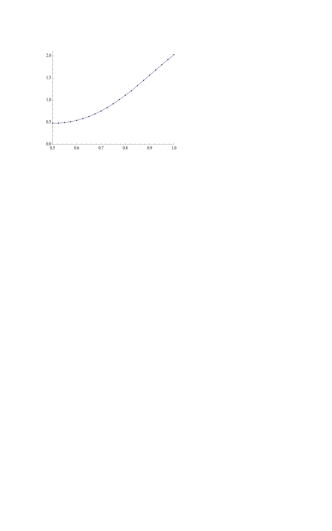
Figure 1: The entanglement coefficient $y=\mathcal{E}(\mu_{1})$, as a function of $x=\mu_{1}:=m_{1}/(m_{1}+m_{2})$, for $0.5\leq\mu_{1}\leq 1.$

We see from Table 1 and Figure 1 that the entanglement coefficient depends strongly in the difference of the masses. It takes its minimun for $\mu_{1}=0.5$, when the masses are equal, and it increases rapidly with the difference of the masses, as $\mu_{1}$ tends to one. This shows that, if the scattering length is fixed, the entanglement takes its minimum when the masses are equal and that it strongly increases with the differences of the masses. This is indeed a remarkable result. Suppose that we consider different pairs of particles that interact in the same way at low energy, in the sense that, to leading order, they have the same total scattering cross section, i.e., such that the scattering length, $c_{0}$, is the same for all the pairs. Moreover, suppose that the total mass, $M$, of the pairs is keep fixed, but that the individual masses, $m_{1},m_{2}$ of the particles are different in each pair. Our results show that, under these conditions, over four times more entanglement is produced by increasing the difference of the masses of the particles in the pairs. In practical terms, this means that in experimental devices to produce entanglement by scattering processes it is advantageous to use particles with a large mass difference.

This fact can be understood in a physically intuitive way as follows: in the scattering of a light particle with a very heavy one, the trajectory of the light particle will be strongly changed, with a large exchange of quantum information between the particles, leading to a large entanglement creation.

Note that in the scattering of a particle with a large mass and a particle with a small mass we can assume that the trajectory of the large particle is not affected by the interaction, i.e. that, to a good approximation, it follows a free trajectory, and that the small particle feels a (external) interaction potential centered in the position of the large particle. However, the trajectory of the small particle will be strongly affected by the interaction, what will produce exchange of information between the particles, leading to the creation of entanglement between them. To evaluate this entanglement it is, however, necessary to take into account the degrees of freedom of both particles, as we do to compute the purity.

In the paper [4] a similar problem is considered in the case of equal masses and spherically symmetric potentials. They give an approximate expression for the leading order of the purity in the case of a Gaussian incoming wave packet that is very narrow in momentum space.

The generation of entanglement in scattering processes has been previously considered in one dimension, mainly for potentials with explicit solution. See [5], [6], and the references quoted there. Moreover, [7], [8], [9], and the references quoted there, consider a system of heavy and light particles. They study the asymptotic dynamics and the decoherence produced on the heavy particles by the scattering with light particles in the limit of small mass ratio, what is different from our problem. The loss of quantum coherence induced on heavy particles by the interaction with light ones has attracted much interest. See for example [10], and [11].

The paper is organized as follows. In Section 2 we define the wave and scattering operators, the scattering matrix and we consider its low-energy behavior. In Section 3 we prove our results in the creation of entanglement. In Section 4 we give our conclusions. In the Appendix we compute integrals that we need in Section 3. Along the paper we denote by $C$ a generic positive constant that does not necessarily have the same value in different appearances.

2 Low-Energy Scattering

We consider the scattering of two spinless particles in three dimensions. We find it convenient to use the time-dependent formalism of scattering theory. See, for example, [13, 14, 15, 16, 17].

The Hilbert space of states in the configuration representation is $\mathcal{H}:=L^{2}({\mathbb{R}}^{6})$. The Schrödinger equation is

$$i\hbar\frac{\partial}{\partial t}\varphi(\mathbf{x}_{1},\mathbf{x}_{2})=H\varphi(\mathbf{x}_{1}.\mathbf{x}_{2}),$$ (2.1)

where the Hamiltonian is given by

$$H=H_{0}+V(\mathbf{x}_{1}-\mathbf{x}_{2}).$$ (2.2)

The operator $H_{0}$ is the free Hamiltonian,

$$H_{0}:=-\frac{\hbar^{2}}{2m_{1}}\Delta_{1}-\frac{\hbar^{2}}{2m_{2}}\Delta_{2},$$ (2.3)

with $\hbar$ Planck’s constant, $m_{j},j=1,2$, respectively, the mass of particle one and two, and $\Delta_{j}$ the Laplacian in the coordinates $\mathbf{x}_{j},j=1,2$. The potential of interaction is multiplication by a real-valued function, $V(\mathbf{x})$, defined for $\mathbf{x}\in{\mathbb{R}}^{3}$. As usual, we assume that the interaction depends on the difference of the coordinates $\mathbf{x}_{1}-\mathbf{x}_{2}$, but no spherical symmetry is supposed. $V$ satisfies the following condition.

ASSUMPTION 2.1.

For some $\beta>0$, $(1+|x|)^{\beta}V(\mathbf{x})$ is a compact operator from the Sobolev space $H^{1}$ into the Sobolev space $H^{-1}$ .

Below we will assume that $\beta>5$ or that $\beta>7$. For the definition of Sobolev’s spaces see [12]. Conditions for Assumption 2.1 to hold are well know [18], [19]. For example, if (1.4, 1.5) are satisfied.

Under this condition $H$ is defined as the quadratic form sum of $H_{0}$ and $V$ and it is a self-adjoint operator.

The wave operators are defined as

$$W_{\pm}:=\hbox{\rm s-lim}_{\pm\infty}\,e^{i\frac{t}{\hbar}H}\,e^{-i\frac{t}{\hbar}H_{0}}.$$

As is well known, under our condition the wave operators exist and are asymptotically complete, i.e. their ranges coincide with the absolutely continuous subspace of $H$. Moreover, the scattering operator,

$$S=W_{+}^{\ast}\,W_{-},$$ (2.4)

is unitary.

Before the scattering, when the particles are far apart from each other and the interaction is weak, the dynamics of the system is well approximated by an incoming solution to the free Schrödinger equation with the potential set to zero,

$$e^{-i\frac{t}{\hbar}H_{0}}\,\varphi_{-},$$

where the incoming asymptotic state $\varphi_{-}$ is the Cauchy data at time zero of the incoming solution to the free Schrödinger equation. When the particles are close to each other, and the potential is strong, the dynamics of the system is given by the solution to the Schrödinger equation,

$$e^{-i\frac{t}{\hbar}H}\,W_{-}\varphi_{-},$$ (2.5)

that is asymptotic to the incoming solution to the free Schrödinger equation as $t\rightarrow-\infty$,

$$\lim_{t\rightarrow-\infty}\left\|e^{-i\frac{t}{\hbar}H_{0}}\,\varphi_{-}-e^{-i\frac{t}{\hbar}H}\,W_{-}\varphi_{-}\right\|=0.$$

After the scattering, for large positive times, the particles again are far away from each other and the dynamics of the system is well approximated by the outgoing solution to the free Schrödinger equation

$$e^{-i\frac{t}{\hbar}H_{0}}\,W_{+}^{\ast}\,W_{-}\varphi_{-},$$

that is asymptotic to the solution to the Schrödinger equation (2.5) as $t\rightarrow\infty$,

$$\lim_{t\rightarrow\infty}\left\|e^{-i\frac{t}{\hbar}H}\,W_{-}\varphi_{-}-e^{-i\frac{t}{\hbar}H_{0}}\,W_{+}^{\ast}\,W_{-}\varphi_{-}\right\|=0.$$

The outgoing asymptotic state is the Cauchy data at time zero of the outgoing solution to the free Schrödinger equation: $\varphi_{+}:=W_{+}^{\ast}\,W_{-}\varphi_{-}$. It is given by the scattering operator, $\varphi_{+}=S\varphi_{-}$.

As usual, we consider the center-of-mass and relative distance coordinates,

$$\mathbf{x}_{\rm cm}:=\frac{m_{1}\mathbf{x}_{1}+m_{2}\mathbf{x}_{2}}{m_{1}+m_{2}},$$ (2.6)

$$\mathbf{x}:=\mathbf{x}_{1}-\mathbf{x}_{2}.$$ (2.7)

The state space $\mathcal{H}$ factorizes under this change of coordinates as,

$$\mathcal{H}={\mathcal{H}}_{\rm cm}\otimes{\mathcal{H}}_{\rm rel},$$ (2.8)

Where ${\mathcal{H}}_{\rm cm}=L^{2}({\mathbb{R}}^{3}),{\mathcal{H}}_{\rm rel}:=L^{2}({\mathbb{R}}^{3})$ are, respectively, the state spaces for the center-of-mass motion and the relative motion. Since the interaction depends only on $\mathbf{x}$, the Hamiltonian and the wave and scattering operators decompose under the tensor product structure and, in particular, we have that

$$S=I_{\rm cm}\otimes S_{rel},$$ (2.9)

where $I_{\rm cm}$ is the identity operator on ${\mathcal{H}}_{\rm cm}$ and $S_{\rm rel}$ is the scattering operator for the relative motion, that is defined as follows. The Hamiltonian for the relative motion is given by,

$$H_{\rm rel}:=-\frac{\hbar^{2}}{2m}\Delta_{\mathbf{x}}+V(\mathbf{x}),$$ (2.10)

where $m$ is the reduced mass,

$$m:=\frac{m_{1}\,m_{2}}{m_{1}+m_{2}},$$ (2.11)

and $\Delta_{\mathbf{x}}$ is the Laplacian in the $\mathbf{x}$ coordinate. The free relative Hamiltonian is,

$$H_{0,\rm rel}:=-\frac{\hbar^{2}}{2m}\Delta_{\mathbf{x}}.$$ (2.12)

The relative wave operators are defined as,

$$W_{\pm\rm,rel}:=\hbox{\rm s-lim}_{\pm\infty}\,e^{i\frac{t}{\hbar}H_{rel}}\,e^{-i\frac{t}{\hbar}H_{0},rel}.$$ (2.13)

The relative scattering operator,

$$S_{\rm rel}=W_{+\rm,rel}^{\ast}\,W_{-\rm,rel},$$ (2.14)

is a unitary operator on ${\mathcal{H}}_{\rm rel}$.

We denote by $\hat{\mathcal{H}}:=L^{2}({\mathbb{R}}^{6})$ the state space in the momentum representation. The momentum of the particles one and two are, respectively, $\mathbf{p}_{1},\mathbf{p}_{2}$. We define the Fourier transform as an unitary operator from $\mathcal{H}$ onto $\hat{\mathcal{H}}$,

$$\mathcal{F}\varphi(\mathbf{p}_{1},\mathbf{p}_{2}):=\frac{1}{(2\pi\hbar)^{3}}\int_{{\mathbb{R}}^{6}}\,e^{-\frac{i}{\hbar}(\mathbf{p}_{1}\cdot\mathbf{x}_{1}+\mathbf{p}_{2}\cdot\mathbf{x}_{2})}\,\varphi(\mathbf{x}_{1},\mathbf{x}_{2}).$$ (2.15)

It is also convenient to take as coordinates in the momentum representation the momentum of the center of mass and the relative momentum,

$$\mathbf{p}_{\rm cm}:=\mathbf{p}_{1}+\mathbf{p}_{2},$$ (2.16)

$$\mathbf{p}:=\frac{m_{2}\mathbf{p}_{1}-m_{1}\mathbf{p}_{2}}{m_{1}+m_{2}}.$$ (2.17)

The state space in the momentum representation also factorizes as a tensor product,

$$\hat{\mathcal{H}}=\hat{\mathcal{H}}_{\rm cm}\otimes\hat{\mathcal{H}}_{\rm rel},$$ (2.18)

where $\hat{\mathcal{H}}_{\rm cm}=L^{2}({\mathbb{R}}^{3}),\hat{\mathcal{H}}_{\rm rel}:=L^{2}({\mathbb{R}}^{3})$ are, respectively, the state spaces in the momentum representation for the center-of-mass motion and the relative motion.

The scattering operator in the momentum representation,

$$\hat{S}:={\mathcal{F}}\,S\,{\mathcal{F}}^{-1},$$ (2.19)

decomposes as,

$$\hat{S}=I_{\rm cm}\otimes\hat{S}_{\rm rel},$$ (2.20)

where $\hat{S}_{\rm rel}$ is the scattering operator for the relative motion in the momentum representation,

$$\hat{S}_{\rm rel}:={\mathcal{F}}_{\rm rel}\,S_{\rm rel}\,{\mathcal{F}}_{\rm rel}^{-1},$$ (2.21)

where ${\mathcal{F}}_{\rm rel}$ is the Fourier transform in the relative coordinate,

$${\mathcal{F}}_{\rm rel}\varphi(\mathbf{p}):=\frac{1}{(2\pi\hbar)^{3/2}}\,\int_{{\mathbb{R}}^{3}}\,e^{-\frac{i}{\hbar}\mathbf{p}\cdot\mathbf{x}}\,\varphi(\mathbf{x}).$$ (2.22)

We denote by ${\mathbb{S}}^{2}$ the unit sphere in ${\mathbb{R}}^{3}$.

As $S_{\rm rel}$ commutes with $H_{\rm 0,rel}$ (energy conservation) we have

$$\left(\hat{S}_{\rm rel}\varphi\right)(\mathbf{p})=\left({\mathcal{S}}(\mathbf{p}^{2}/2m)\varphi\right)(\mathbf{p}),$$ (2.23)

where the scattering matrix, ${\mathcal{S}}(E)$, is a unitary operator in $L^{2}({\mathbb{S}}^{2})$ for each $E\in(0,\infty)$. Note that the scattering matrix defined in the time-dependent framework coincides with the scattering matrix defined in the stationary theory by means of the solutions to the Lippmann-Schwinger equations.

The following theorem has been proved by Kato and Jensen [19]. Note that they consider the case $\hbar=1,m=1/2$ but the general case is easily obtained by an elementary argument. A zero energy resonance (half-bound state) is a solution to $H_{\mathrm{r}el}\varphi=0$ that decays at infinity, but that is not in $L^{2}({\mathbb{R}}^{3})$. See [19] for a precise definition. For generic potentials $V$ there is neither a resonance nor an eigenvalue at zero for $H_{\mathrm{r}el}$. That is to say, if we consider the potential $\lambda V$ with a coupling constant $\lambda$, zero can be a resonance and/or an eigenvalue for at most a finite or denumerable set of $\lambda$’s without any finite accumulation point.

The scattering length is defined as,

$$c_{0}:=\frac{1}{4\pi}\,\left(\frac{2m}{\hbar^{2}}V\,(1+G_{0}\frac{2m}{\hbar^{2}}V)^{-1}1,1\right),$$ (2.24)

where $(.,.)$ is the $L^{2}$ scalar product in ${\mathbb{R}}^{3}$, $1$ designates the function identically equal to one and $G_{0}$ is the operator with integral kernel the Green’s function at zero energy,

$$G_{0}(\mathbf{x},\mathbf{y}):=\frac{1}{4\pi|\mathbf{x}-\mathbf{y}|},\mathbf{x},\mathbf{y}\in{\mathbb{R}}^{3}.$$ (2.25)

The operator $(1+G_{0}\frac{2m}{\hbar^{2}}V)$ is invertible because zero is neither an eigenvalue nor a resonance for $H_{\mathrm{r}el}$. We define the scattering length, $c_{0}$, with the opposite sign to the one used in [19], in order that it coincides with the definition used in the physics literature [16, 17]. Furthermore,

$$Y_{0}(\nu):=\frac{1}{\sqrt{4\pi}},\nu\in{\mathbb{S}}^{2},$$ (2.26)

$$Y_{1}(\nu):=\frac{1}{4\pi^{3/2}}\,\left(\frac{2m}{\hbar^{2}}V\,\left(1+G_{0}\frac{2m}{\hbar^{2}}V\right)^{-1}1,\mathbf{x}\cdot\nu\right),\nu\in{\mathbb{S}}^{2}.$$ (2.27)

We denote by ${\mathcal{B}}\left(L^{2}({\mathbb{S}}^{2})\right)$ the Banach space of all bounded linear operators on $L^{2}({\mathbb{S}}^{2})$.

THEOREM 2.2.

(Kato and Jensen [19]) Suposse that Assumption 2.1 is satisfied and that at zero $H_{\mathrm{r}el}$ has neither a resonance (half-bound state) nor an eigenvalue. Then, If $\beta>5$, in the norm of ${\mathcal{B}}\left(L^{2}({\mathbb{S}}^{2})\right)$ we have for $|\mathbf{p}/\hbar|\rightarrow 0$ the expansion,

$${\mathcal{S}}(\mathbf{p}^{2}/2m)=I+i|\mathbf{p}/\hbar|\,\Sigma^{0}_{1}-|\mathbf{p}/\hbar|^{2}\,\Sigma^{0}_{2}+o(|\mathbf{p}/\hbar|^{2}),$$ (2.28)

where $I$ is the identity operator on $L^{2}({\mathbb{S}}^{2})$,

$$\Sigma^{0}_{1}:=-2c_{0}\left(\cdot,Y_{0}\right)\,Y_{0},$$ (2.29)

and

$$\Sigma^{0}_{2}:=2c_{0}^{2}\left(\cdot,Y_{0}\right)\,Y_{0}+\left(\cdot,Y_{1}\right)Y_{0}-\left(\cdot,Y_{0}\right)Y_{1}.$$ (2.30)

Furthermore, if $\beta>7,o(|\mathbf{p}/\hbar|^{2})$ can be replaced by $O(|\mathbf{p}/\hbar|^{3})$.

Note that $Y_{1}=0$ if $V$ is spherically symmetric. We see that, as is well known, the leading order at low energy of ${\mathcal{S}}(\mathbf{p}^{2}/2m)-I$ is given by the scattering length, i.e. in leading order the scattering is isotropic. The anisotropic effects appear at second order.

3 Entanglement Creation

Consider a pure state of the two-particle system given in the momentum representation by the wave function $\varphi(\mathbf{p}_{1},\mathbf{p}_{2})$. Let us denote by $\rho(\varphi)$ the one-particle reduced density matrix with integral kernel,

$$\rho(\varphi)(\mathbf{p}_{1},\mathbf{p}_{1}^{\prime}):=\int\varphi(\mathbf{p}_{1},\mathbf{p}_{2})\,\overline{\varphi(\mathbf{p}_{1}^{\prime},\mathbf{p}_{2})}\,\,d\mathbf{p}_{2},$$

and by ${\mathcal{P}}(\varphi)$ the purity,

$${\mathcal{P}}(\varphi):=\hbox{\rm Tr}(\rho^{2})=\int_{{\mathbb{R}}^{12}}\,d\mathbf{p}_{1}\,d\mathbf{p}_{1}^{\prime}\,d\mathbf{p}_{2}\,d\mathbf{p}_{2}^{\prime}\,\varphi(\mathbf{p}_{1},\mathbf{p}_{2})\,\overline{\varphi(\mathbf{p}_{1}^{\prime},\mathbf{p}_{2})}\,\varphi(\mathbf{p}_{1}^{\prime},\mathbf{p}_{2}^{\prime})\,\overline{\varphi(\mathbf{p}_{1},\mathbf{p}_{2}^{\prime})}.$$ (3.1)

The purity is an entanglement measure that is closely related to the Rényi entropy of order $2$,$-\hbox{\rm ln Tr}(\rho^{2})$ [3, 20, 21]. It is trivially related to the linear entropy, $S_{L}$, as $S_{L}=1-\mathcal{P}$. It satisfies $0\leq\mathcal{P}\leq 1$ if $\varphi$ is normalized to one. Furthermore, it is equal to one for a product state, $\varphi=\varphi_{1}(\mathbf{p}_{1})\,\varphi_{2}(\mathbf{p}_{2})$. The purity is an entanglement measure that is convenient for the study of entanglement creation in scattering processes because it can be directly computed in terms of the scattering matrix.

We work in the center-of-mass frame and we consider an incoming asymptotic state that is a product of two normalized Gaussian wave functions,

$$\varphi_{\rm in,\mathbf{p}_{0}}(\mathbf{p}_{1},\mathbf{p}_{2}):=\varphi_{\mathbf{p}_{0}}(\mathbf{p}_{1})\,\varphi_{-\mathbf{p}_{0}}(\mathbf{p}_{2}),$$ (3.2)

where

$$\varphi_{\mathbf{p}_{0}}(\mathbf{p}_{1}):=\frac{1}{(\sigma^{2}\pi)^{3/4}}e^{-(\mathbf{p}_{1}-\mathbf{p}_{0})^{2}/2\sigma^{2}}.$$ (3.3)

In the incoming asymptotic state (3.2) particle one has mean momentum $\mathbf{p}_{0}$ and particle two has mean momentum $-\mathbf{p}_{0}$. The variance of the momentum distribution of both particles is $\sigma$. We assume that the scattering takes place at the origin at time zero, and for this reason the average position of both particles is zero in the incoming asymptotic state (3.2). Note that by (2.17) the mean value of the relative momentum in the state (3.2) is equal to $\mathbf{p}_{0}$.

Since $\varphi_{\rm in,\mathbf{p}_{0}}$ is a product state its purity is one,

$$\mathcal{P}(\varphi_{\rm in,\mathbf{p}_{0}})=1.$$ (3.4)

After the scattering process is over the two particles are in the outgoing asymptotic state, $\varphi_{\rm out,\mathbf{p}_{0}}$, given by

$$\varphi_{\rm out,\mathbf{p}_{0}}(\mathbf{p}_{1},\mathbf{p}_{2}):=\left(\mathcal{S}(\mathbf{p}^{2}/2m)\varphi_{\rm in,\mathbf{p}_{0}}\right)(\mathbf{p}_{1},\mathbf{p}_{2}).$$ (3.5)

Since the relative momentum, $\mathbf{p}$, depends on $\mathbf{p}_{1}$ and on $\mathbf{p}_{2}$, $\varphi_{\rm out,\mathbf{p}_{0}}$ is no longer a product state and it has purity smaller than one, what means that entanglement between the two particles has been created by the scattering process.

We will rigorously compute the leading order of the purity of $\varphi_{\rm out,\mathbf{p}_{0}}$ -in a quantitative way- in the low-energy limit for the relative motion. Note that to be in the low-energy regime we need that the mean relative momentum $\mathbf{p}_{0}$ be small, but also that the variance $\sigma$ be small, because if $\sigma$ is large the incoming asymptotic state $\varphi_{\rm in,\mathbf{p}_{0}}$ will have a big probability of having large momentum, even if the mean relative momentum $\mathbf{p}_{0}$ is small.

We first introduce some notations that we need.

We denote by $\varphi_{\rm in}$ the incoming asymptotic state with mean value of the relative momentum zero,

$$\varphi_{\rm in}(\mathbf{p}_{1},\mathbf{p}_{2}):=\varphi(\mathbf{p}_{1})\,\varphi(\mathbf{p}_{2}),$$ (3.6)

where,

$$\varphi(\mathbf{p}):=\frac{1}{(\sigma^{2}\pi)^{3/4}}e^{-\mathbf{p}^{2}/2\sigma^{2}},\mathbf{p}\in{\mathbb{R}}^{3},$$ (3.7)

and by $\varphi_{\rm out}$ the outgoing asymptotic state with incoming asymptotic state $\varphi_{\rm in}$,

$$\varphi_{\rm out}(\mathbf{p}_{1},\mathbf{p}_{2}):=\left(\mathcal{S}(\mathbf{p}^{2}/2m)\varphi_{\rm in}\right)(\mathbf{p}_{1},\mathbf{p}_{2}).$$ (3.8)

We define,

$$\psi_{\mathbf{q}_{0}}(\mathbf{q}):=\frac{1}{(\pi)^{3/4}}e^{-(\mathbf{q}-\mathbf{q}_{0})^{2}/2},\mathbf{q}\in{\mathbb{R}}^{3},$$ (3.9)

$$\psi(\mathbf{q}):=\frac{1}{(\pi)^{3/4}}e^{-\mathbf{q}^{2}/2},\mathbf{q}\in{\mathbb{R}}^{3},$$ (3.10)

$$\psi_{\rm in,\mathbf{q}_{0}}(\mathbf{q}_{1},\mathbf{q}_{2}):=\psi_{\mathbf{q}_{0}}(\mathbf{q}_{1})\,\psi_{-\mathbf{q}_{0}}(\mathbf{q}_{2}),$$ (3.11)

$$\psi_{\rm in}(\mathbf{q}_{1},\mathbf{q}_{2}):=\psi(\mathbf{q}_{1})\,\psi(\mathbf{q}_{2}).$$ (3.12)

We prepare the following proposition that we need later.

PROPOSITION 3.1.

$$\left\|\varphi_{\rm in,\mathbf{p}_{0}}-\varphi_{\rm in}\right\|\leq C\,\hbox{\rm min}\{|\mathbf{p}_{0}|/\sigma,1\},$$ (3.13)

$$\left\|\mathbf{p}\left(\varphi_{\rm in,\mathbf{p}_{0}}-\varphi_{\rm in}\right)\right\|\leq C\,|\mathbf{p}_{0}|.$$ (3.14)

Proof: We denote $\mathbf{q}_{0}:=\mathbf{p}_{0}/\sigma.$ Then,

$$\left\|\varphi_{\rm in,\mathbf{p}_{0}}-\varphi_{\rm in}\right\|=\left\|\psi_{\rm in,\mathbf{q}_{0}}-\psi_{\rm in}\right\|.$$ (3.15)

Assume first that $|\mathbf{q}_{0}|\leq 1$. We have that,

$$\psi_{\rm in,\mathbf{q}_{0}}-\psi_{\rm in}=\frac{1}{\pi^{3/2}}\,e^{-(\mathbf{q}_{1}^{2}+\mathbf{q}_{2}^{2})/2}\left(e^{-\mathbf{q}_{0}^{2}+(\mathbf{q}_{1}-\mathbf{q}_{2})\cdot\mathbf{q}_{0}}-1\right).$$ (3.16)

Moreover,

$$\left|e^{-\mathbf{q}_{0}^{2}+(\mathbf{q}_{1}-\mathbf{q}_{2})\cdot\mathbf{q}_{0}}-1\right|=\left|\int_{0}^{-\mathbf{q}_{0}^{2}+(\mathbf{q}_{1}-\mathbf{q}_{2})\cdot\mathbf{q}_{0}}\,e^{s}\,ds\right|\leq$$ (3.17)

$$e^{|\mathbf{q}_{0}|^{2}+|\mathbf{q}_{0}|(|\mathbf{q}_{1}|+|\mathbf{q}_{2}|)}(|\mathbf{q}_{0}|^{2}+|\mathbf{q}_{0}|(|\mathbf{q}_{1}|+|\mathbf{q}_{2}|)).$$ (3.18)

It follows from (3.15,3.16, and 3.18) that (3.13) holds for $\mathbf{q}_{0}|\leq 1$. In the case $|\mathbf{q}_{0}|\geq 1$ the estimate is immediate because,

$$\left\|\varphi_{\rm in,\mathbf{p}_{0}}-\varphi_{\rm in}\right\|\leq 2.$$

Note that by (2.17),

$$|\mathbf{p}|\leq|\mathbf{p}_{1}|+|\mathbf{p}_{2}|.$$

Then, if $|\mathbf{q}_{0}|\leq 1$ as in the proof of (3.13) we prove that,

$$\left\|\mathbf{p}\left(\varphi_{\rm in,\mathbf{p}_{0}}-\varphi_{\rm in}\right)\right\|\leq C\,|\mathbf{p}_{0}|.$$ (3.19)

If $|\mathbf{q}_{0}|\geq 1$ we estimate as follows,

$$\left\|\mathbf{p}\left(\varphi_{\rm in,\mathbf{p}_{0}}-\varphi_{\rm in}\right)\right\|\leq\left\||\mathbf{p}_{1}|\left(\varphi_{\rm in,\mathbf{p}_{0}}-\varphi_{\rm in}\right)\right\|+\left\||\mathbf{p}_{2}|\left(\varphi_{\rm in,\mathbf{p}_{0}}-\varphi_{\rm in}\right)\right\|.$$ (3.20)

Furthermore,

$$\left\||\mathbf{p}_{1}|\,\left(\varphi_{\rm in,\mathbf{p}_{0}}-\varphi_{\rm in}\right)\right\|\leq\left\||\mathbf{p}_{1}-\mathbf{p}_{0}|\,\varphi_{\rm in,\mathbf{p}_{0}}\right\|+\left\||\mathbf{p}_{0}|\,\varphi_{\rm in,\mathbf{p}_{0}}\right\|+\left\||\mathbf{p}_{1}|\,\varphi_{\rm in}\right\|\leq$$

$$\sigma\left\||\mathbf{q}_{1}-\mathbf{q}_{0}|\,\psi_{\rm in,\mathbf{q}_{0}}\right\|+|\mathbf{p}_{0}|+\sigma\left\||\mathbf{q}_{1}|\,\psi_{\rm in}\right\|\ \leq C|\mathbf{p}_{0}|.$$ (3.21)

In the last inequality we used that $\sigma\leq|\mathbf{p}_{0}|$. In the same way we prove that,

$$\left\||\mathbf{p}_{2}|\left(\varphi_{\rm in,\mathbf{p}_{0}}-\varphi_{\rm in}\right)\right\|\leq C|\mathbf{p}_{0}|.$$ (3.22)

By (3.20, 3, 3.22) we have that,

$$\left\|\mathbf{p}\left(\varphi_{\rm in,\mathbf{p}_{0}}-\varphi_{\rm in}\right)\right\|\leq C|\mathbf{p}_{0}|.$$ (3.23)

Equation (3.14) follows from (3.19) and (3.23).

$\Box$

Let us denote,

$$\mathcal{T}(\mathbf{p}^{2}/2m):=\mathcal{S}(\mathbf{p}^{2}/m)-I,$$ (3.24)

where $I$ designates the identity operator on $L^{2}({\mathbb{S}}^{2})$. It follows from (2.28) and since $\|\mathcal{S}(\mathbf{p}^{2}/2m)\|_{\mathcal{B}(L^{2}({\mathbb{S}}^{2}))}=1$, that

$$\left\|\mathcal{T}(\mathbf{p}^{2}/2m)\right\|_{\mathcal{B}(L^{2}({\mathbb{S}}^{2}))}\leq C\frac{|\mathbf{p}/\hbar|}{1+|\mathbf{p}/\hbar|}.$$ (3.25)

Hence,

$$\left\|\mathcal{T}(\mathbf{p}^{2}/2m)\varphi_{\rm in}\right\|\leq C\frac{\sigma}{\hbar}\left\|\mathcal{\mathbf{q}}\,\psi_{\rm in}\right\|.$$ (3.26)

We designate,

$$\mathcal{L}(\phi_{1},\phi_{2},\phi_{3},\phi_{4}):=\int_{{\mathbb{R}}^{12}}\,d\mathbf{p}_{1}\,d\mathbf{p}_{1}^{\prime}\,d\mathbf{p}_{2}\,d\mathbf{p}_{2}^{\prime}\,\phi_{1}(\mathbf{p}_{1},\mathbf{p}_{2})\,\overline{\phi_{2}(\mathbf{p}_{1}^{\prime},\mathbf{p}_{2})}\,\phi_{3}(\mathbf{p}_{1}^{\prime},\mathbf{p}_{2}^{\prime})\,\overline{\phi_{4}(\mathbf{p}_{1},\mathbf{p}_{2}^{\prime})}.$$ (3.27)

Note that,

$$\mathcal{P}(\phi)=\mathcal{L}(\phi,\phi,\phi,\phi).$$

It follows from the Schwarz inequality that,

$$\left|{\mathcal{L}}(\phi_{1},\phi_{2},\phi_{3},\phi_{4})\right|\leq\Pi_{j=1}^{4}\|\phi_{j}\|.$$ (3.28)

The following theorem is our first low-energy estimate of the purity.

THEOREM 3.2.

Suposse that Assumption 2.1 is satisfied and that at zero $H_{\mathrm{r}el}$ has neither a resonance (half-bound state) nor an eigenvalue. Then,

$$\mathcal{P}(\varphi_{\rm out,\mathbf{p}_{0}})=\mathcal{P}(\varphi_{\rm out})+O(|\mathbf{p}_{0}/\hbar|),\hbox{\rm as}\,|\mathbf{p}_{0}/\hbar|\rightarrow 0,$$ (3.29)

where $O(|\mathbf{p}_{0}/\hbar|)$ is uniform on $\sigma$, for $\sigma$ in bounded sets.

Proof: Writing $\varphi_{\rm out,\mathbf{p}_{0}}$ as,

$$\varphi_{\rm out,\mathbf{p}_{0}}:=\mathcal{S}(\mathbf{p}^{2}/2m)\varphi_{\rm in,\mathbf{p}_{0}}=\varphi_{\rm in,\mathbf{p}_{0}}+\mathcal{T}(\mathbf{p}^{2}/2m)\varphi_{\rm in,\mathbf{p}_{0}},$$

and using (3.4), we see that we can write $\mathcal{P}(\varphi_{\rm out,\mathbf{p}_{0}})$ as follows,

$$\mathcal{P}(\varphi_{\rm out,\mathbf{p}_{0}})=1+\mathcal{R}(\mathbf{p}_{0}),$$ (3.30)

where $\mathcal{R}(\mathbf{p}_{0})$ is given by,

$$\mathcal{R}(\mathbf{p}_{0}):=\sum_{i=1}^{A}\mathcal{L}_{i}(\mathbf{p}_{0},\psi_{1},\psi_{2},\psi_{3},\psi_{4}),$$ (3.31)

for some integer $A$, and where each of the $\mathcal{L}_{i}(\mathbf{p}_{0},\psi_{1},\psi_{2},\psi_{3},\psi_{4})$ is equal to,

$$\mathcal{L}_{i}(\mathbf{p}_{0},\psi_{1},\psi_{2},\psi_{3},\psi_{4})=\mathcal{L}(\psi_{1},\psi_{2},\psi_{3},\psi_{4}),$$ (3.32)

where for some $1\leq k\leq 4$, $k$ of the $\psi_{j}$ are equal to $\mathcal{T}(\mathbf{p}^{2}/2m)\varphi_{\rm in,\mathbf{p}_{0}}$ and the remaining $4-k$ are equal to $\varphi_{\rm in,\mathbf{p}_{0}}$. Similarly,

$$\mathcal{P}(\varphi_{\rm out})=1+\mathcal{R}(0),$$ (3.33)

with

$$\mathcal{R}(0):=\sum_{i=1}^{A}\mathcal{L}_{i}(0,\psi_{1},\psi_{2},\psi_{3},\psi_{4}).$$ (3.34)

Below we prove that,

$$\mathcal{R}(\mathbf{p}_{0})=\mathcal{R}(0)+O(|\mathbf{p}_{0}/\hbar|),\hbox{\rm as}\,|\mathbf{p}_{0}/\hbar|\rightarrow 0,$$ (3.35)

what proves the theorem in view of (3.30,3.33).

We proceed to prove (3.35). Without losing generality we can assume that,

$$\mathcal{L}_{1}(\mathbf{p}_{0},\psi_{1},\psi_{2},\psi_{3},\psi_{4})=\mathcal{L}(\mathcal{T}(\mathbf{p}^{2}/2m)\varphi_{\rm in,\mathbf{p}_{0}},\varphi_{\rm in,\mathbf{p}_{0}},\varphi_{\rm in,\mathbf{p}_{0}},\varphi_{\rm in,\mathbf{p}_{0}}).$$ (3.36)

We have that,

$$\mathcal{L}_{1}(\mathbf{p}_{0},\psi_{1},\psi_{2},\psi_{3},\psi_{4})=\mathcal{L}(\mathcal{T}(\mathbf{p}^{2}/2m)\varphi_{\rm in},\varphi_{\rm in,\mathbf{p}_{0}},\varphi_{\rm in,\mathbf{p}_{0}},\varphi_{\rm in,\mathbf{p}_{0}})+\mathcal{L}(\mathcal{T}(\mathbf{p}^{2}/2m)(\varphi_{\rm in,\mathbf{p}_{0}}-\varphi_{\rm in}),\varphi_{\rm in,\mathbf{p}_{0}},\varphi_{\rm in,\mathbf{p}_{0}},\varphi_{\rm in,\mathbf{p}_{0}}).$$ (3.37)

By (3.14, 3.25, 3.28, 3.37),

$$\mathcal{L}_{1}(\mathbf{p}_{0},\psi_{1},\psi_{2},\psi_{3},\psi_{4})=\mathcal{L}(\mathcal{T}(\mathbf{p}^{2}/2m)\varphi_{\rm in},\varphi_{\rm in,\mathbf{p}_{0}},\varphi_{\rm in,\mathbf{p}_{0}},\varphi_{\rm in,\mathbf{p}_{0}})+O(|\mathbf{p}_{0}/\hbar|),\hbox{\rm as}\,|\mathbf{p}_{0}/\hbar|\rightarrow 0.$$ (3.38)

In the same way, using (3.13, 3.26,3.38), we prove that,

$$\mathcal{L}_{1}(\mathbf{p}_{0},\psi_{1},\psi_{2},\psi_{3},\psi_{4})=\mathcal{L}(\mathcal{T}(\mathbf{p}^{2}/2m)\varphi_{\rm in},\varphi_{\rm in},\varphi_{\rm in,\mathbf{p}_{0}},\varphi_{\rm in,\mathbf{p}_{0}})+O(|\mathbf{p}_{0}/\hbar|),\hbox{\rm as}\,|\mathbf{p}_{0}/\hbar|\rightarrow 0.$$ (3.39)

Repeating this argument two more times we obtain that,

$$\mathcal{L}_{1}(\mathbf{p}_{0},\psi_{1},\psi_{2},\psi_{3},\psi_{4})=\mathcal{L}(\mathcal{T}(\mathbf{p}^{2}/2m)\varphi_{\rm in},\varphi_{\rm in},\varphi_{\rm in},\varphi_{\rm in,})+O(|\mathbf{p}_{0}/\hbar|)=$$

$$\mathcal{L}_{1}(0,\psi_{1},\psi_{2},\psi_{3},\psi_{4})+O(|\mathbf{p}_{0}/\hbar|),\hbox{\rm as}\,|\mathbf{p}_{0}/\hbar|\rightarrow 0.$$ (3.40)

We prove in the same way that,

$$\mathcal{L}_{j}(\mathbf{p}_{0},\psi_{1},\psi_{2},\psi_{3},\psi_{4})=\mathcal{L}_{j}(0,\psi_{1},\psi_{2},\psi_{3},\psi_{4})+O(|\mathbf{p}_{0}/\hbar|),2\leq j\leq A,\hbox{\rm as}\,|\mathbf{p}_{0}/\hbar|\rightarrow 0.$$ (3.41)

Equation (3.35) follows from (3.30,3.31,3.33,3.34, 3.40,3.41).

$\Box$

We now compute the leading order of the purity of $\varphi_{\rm out}$.

We denote,

$$\mathcal{T}_{1}(\mathbf{p}^{2}/2m):={\mathcal{S}}(\mathbf{p}^{2}/2m)-I-i|\mathbf{p}/\hbar|\,\Sigma^{0}_{1}+|\mathbf{p}/\hbar|^{2}\,\Sigma^{0}_{2}.$$ (3.42)

It follows from Theorem 2.2 that,

$$\left\|\mathcal{T}_{1}(\mathbf{p}^{2}/m)\right\|_{\mathcal{B}(L^{2}({\mathbb{S}}^{2}))}\leq\left\{\begin{array}[]{clcr}|\mathbf{p}/\hbar|^{2}o(1),&\hbox{\rm if}\,\beta>5,\\ |\mathbf{p}/\hbar|^{2}O(|\mathbf{p}/\hbar|),&\hbox{\rm if}\,\beta>7,\end{array}\right.$$ (3.43)

where $o(1)$ and $O(|\mathbf{p}/\hbar|)$ are bounded functions of $|\mathbf{p}/\hbar|$, $\lim_{|\mathbf{p}/\hbar|\rightarrow 0}o(1)=0$ and $O(|\mathbf{p}/\hbar|)\leq C|\mathbf{p}/\hbar|$ for $|\mathbf{p}/\hbar|\leq 1$.

THEOREM 3.3.

Suposse that Assumption 2.1 is satisfied and that at zero $H_{\mathrm{r}el}$ has neither a resonance (half-bound state) nor an eigenvalue. Then, as $\sigma/\hbar$ goes to zero,

$$\mathcal{P}(\varphi_{\rm out})=\mathcal{P}\left(\left[I+i|\mathbf{p}/\hbar|\,\Sigma^{0}_{1}-|\mathbf{p}/\hbar|^{2}\,\Sigma^{0}_{2}\right]\varphi_{\rm in}\right)+\left\{\begin{array}[]{clcr}o\left(|\sigma/\hbar|^{2}\right),&\hbox{\rm if}\,\beta>5,\\ O\left(|\sigma/\hbar|^{3}\right),&\hbox{\rm if}\,\beta>7.\end{array}\right.$$ (3.44)

Proof: We write $\varphi_{\rm out}$ as follows,

$$\varphi_{\rm out}=\varphi_{\rm out,1}+\mathcal{T}_{1}(\mathbf{p}^{2}/2m)\varphi_{\rm in},$$

where,

$$\varphi_{\rm out,1}:=\left[I+i|\mathbf{p}/\hbar|\,\Sigma^{0}_{1}-|\mathbf{p}/\hbar|^{2}\,\Sigma^{0}_{2}\right]\varphi_{\rm in}.$$ (3.45)

Using this decomposition we write $\mathcal{P}(\varphi_{\rm out})$ as follows,

$$\mathcal{P}(\varphi_{\rm out})=\mathcal{P}(\varphi_{\rm out,1})+\mathcal{R}(\sigma),$$ (3.46)

where $\mathcal{R}(\sigma)$ is given by,

$$\mathcal{R}(\sigma):=\sum_{i=1}^{B}\mathcal{L}_{i}(\sigma,\psi_{1},\psi_{2},\psi_{3},\psi_{4}),$$ (3.47)

for some integer $B$, and where each of the $\mathcal{L}_{i}(\sigma,\psi_{1},\psi_{2},\psi_{3},\psi_{4})$ is equal to,

$$\mathcal{L}_{i}(\sigma,\psi_{1},\psi_{2},\psi_{3},\psi_{4})=\mathcal{L}(\psi_{1},\psi_{2},\psi_{3},\psi_{4}),$$ (3.48)

where for some $1\leq k\leq 4$, $k$ of the $\psi_{j}$ are equal to $\varphi_{\rm out,1}$ and the remaining $4-k$ are equal to $\mathcal{T}_{1}(\mathbf{p}^{2}/2m)\varphi_{\rm in}$.

We proceed to prove that as $\sigma/\hbar$ goes to zero,

$$\mathcal{R}(\sigma)=\left\{\begin{array}[]{clcr}o\left(|\sigma/\hbar|^{2}\right),&\hbox{\rm if}\,\beta>5,\\ O\left(|\sigma/\hbar|^{3}\right),&\hbox{\rm if}\,\beta>7,\end{array}\right.$$ (3.49)

what proves the theorem in view of ( 3.46).

Without any loss of generality we can assume that,

$$\mathcal{L}_{B}(\sigma,\psi_{1},\psi_{2},\psi_{3},\psi_{4})=\mathcal{L}(\varphi_{\rm out,1},\varphi_{\rm out,1},\varphi_{\rm out,1},\mathcal{T}_{1}(\mathbf{p}^{2}/2m)\varphi_{\rm in}).$$ (3.50)

By (3.28, 3.43) We have that,

$$\mathcal{L}_{B}(\sigma,\psi_{1},\psi_{2},\psi_{3},\psi_{4})=\left\{\begin{array}[]{clcr}o\left(|\sigma/\hbar|^{2}\right),&\hbox{\rm if}\,\beta>5,\\ O\left(|\sigma/\hbar|^{3}\right),&\hbox{\rm if}\,\beta>7.\end{array}\right.$$ (3.51)

We complete the proof of (3.49) estimating the remaining terms in (3.47) in the same way.

$\Box$

We denote by

$$\mu_{i}=\frac{m_{i}}{m_{1}+m_{2}},i=1,2,$$ (3.52)

the ratio of the mass of the $i$ particle to the total mass.

It follows from (2.16,2.17) that,

$$\mathbf{p}_{1}=\mu_{1}\mathbf{p}_{\rm cm}+\mathbf{p},$$ (3.53)

$$\mathbf{p}_{2}=\mu_{2}\mathbf{p}_{\rm cm}-\mathbf{p},$$ (3.54)

and that,

$$\varphi_{\rm in}=\frac{1}{(\sigma^{2}\pi)^{3/2}}\,\,\displaystyle e^{-\frac{\mu_{1}^{2}+\mu_{2}^{2}}{2\sigma^{2}}\mathbf{p}_{\rm cm}^{2}}\,\,\displaystyle e^{-\frac{\mathbf{p}^{2}+(\mu_{1}-\mu_{2})\mathbf{p}_{\rm cm}\cdot\mathbf{p}}{\sigma^{2}}}.$$ (3.55)

By a simple computation using (3.45, 3.53-3.55) we prove that,

$$\mathcal{P}\left(\left[I+i|\mathbf{p}/\hbar|\,\Sigma^{0}_{1}-|\mathbf{p}/\hbar|^{2}\,\Sigma^{0}_{2}\right]\varphi_{\rm in}\right)=1-(\sigma/\hbar)^{2}\left(\mathcal{P}_{1}(\psi_{\rm in})+\mathcal{P}_{2}(\psi_{\rm in})\right)+O((\sigma/\hbar)^{3}),\quad\hbox{\rm as}\,\sigma/\hbar\rightarrow 0,$$ (3.56)

where,

$$\mathcal{P}_{1}(\psi_{\rm in})=\Sigma_{j=1}^{3}\mathcal{P}_{1,j}(\psi_{\rm in}),$$ (3.57)

with

$$\mathcal{P}_{1,1}(\psi_{\rm in})=-2\int d\mathbf{q}_{1}d\mathbf{q}_{2}d\mathbf{q}_{3}\,|\mu_{2}\mathbf{q}_{1}-\mu_{1}\mathbf{q}_{2}|\,|\mu_{2}\mathbf{q}_{3}-\mu_{1}\mathbf{q}_{2}|\,(\Sigma^{0}_{1}\psi(\mathbf{q}_{1},\mathbf{q}_{2}))\,(\Sigma^{0}_{1}\psi(\mathbf{q}_{3},\mathbf{q}_{2}))\,\psi(\mathbf{q}_{1},\mathbf{q}_{3}),$$ (3.58)

$$\mathcal{P}_{1,2}(\psi_{\rm in})=-2\int d\mathbf{q}_{1}d\mathbf{q}_{2}d\mathbf{q}_{3}\,|\mu_{2}\mathbf{q}_{1}-\mu_{1}\mathbf{q}_{2}|\,|\mu_{2}\mathbf{q}_{1}-\mu_{1}\mathbf{q}_{3}|\,\left(\Sigma^{0}_{1}\psi(\mathbf{q}_{1},\mathbf{q}_{2})\right)\,\left(\Sigma^{0}_{1}\psi(\mathbf{q}_{1},\mathbf{q}_{3})\right)\psi(\mathbf{q}_{2},\mathbf{q}_{3}),$$ (3.59)

$$\mathcal{P}_{1,3}(\psi_{\rm in})=2\left[\int d\mathbf{q}_{1}d\mathbf{q}_{2}\,|\mu_{2}\mathbf{q}_{1}-\mu_{1}\mathbf{q}_{2}|\,\left(\Sigma^{0}_{1}\psi(\mathbf{q}_{1},\mathbf{q}_{2})\right)\,\psi(\mathbf{q}_{1},\mathbf{q}_{2})\right]^{2},$$ (3.60)

and

$$\mathcal{P}_{2}(\psi_{\rm in})=4\int d\mathbf{q}_{1}d\mathbf{q}_{2}\,|\mu_{2}\mathbf{q}_{1}-\mu_{1}\mathbf{q}_{2}|^{2}\,\left(\Sigma^{0}_{2}\psi(\mathbf{q}_{1},\mathbf{q}_{2})\right)\,\psi(\mathbf{q}_{1},\mathbf{q}_{2}).$$ (3.61)

Explicitly evaluating the integrals in (3.58), 3.59,3.60) using (3.55) and $\mu_{2}=1-\mu_{1}$, we prove that,

$$\mathcal{P}_{1,1}(\psi_{\rm in})=-8\frac{c_{0}^{2}\sigma^{2}}{\hbar^{2}}\,J(\mu_{1},1-\mu_{1}),$$ (3.62)

$$\mathcal{P}_{1,2}(\psi_{\rm in})=-8\frac{c_{0}^{2}\sigma^{2}}{\hbar^{2}}\,J(1-\mu_{1},\mu_{1}),$$ (3.63)

$$\mathcal{P}_{1,3}(\psi_{\rm in})=8\frac{c_{0}^{2}\sigma^{2}}{\hbar^{2}}\,\left(L(\mu_{1},1-\mu_{1})\right)^{2},$$ (3.64)

where,

$$\begin{array}[]{c}J(\mu_{1},\mu_{2}):=\frac{1}{\pi^{9/2}}\,\int d\mathbf{q}_{2}\left[\,\,\int d\mathbf{q}_{1}|\mu_{2}\mathbf{q}_{1}-\mu_{1}\mathbf{q}_{2}|\,\,\hbox{\rm Exp}[-\frac{1}{2}(\mu_{1}^{2}+\mu_{2}^{2})(\mathbf{q}_{1}+\mathbf{q}_{2})^{2}-(\mu_{2}\mathbf{q}_{1}-\mu_{1}\mathbf{q}_{2})^{2}-\mathbf{q}_{1}^{2}/2]\right.\\ \\ \left.\displaystyle\frac{\sinh[(\mu_{1}-\mu_{2})\,|\mathbf{q}_{1}+\mathbf{q}_{2}|\,|\mu_{2}\mathbf{q}_{1}-\mu_{1}\mathbf{q}_{2}|]}{(\mu_{1}-\mu_{2})\,|\mathbf{q}_{1}+\mathbf{q}_{2}|\,|\mu_{2}\mathbf{q}_{1}-\mu_{1}\mathbf{q}_{2}|}\,\,\right]^{2},\end{array}$$ (3.65)

and

$$\begin{array}[]{c}L(\mu_{1},\mu_{2}):=\frac{1}{\pi^{3}}\,\int d\mathbf{q}_{1}\,d\mathbf{q}_{2}|\mu_{2}\mathbf{q}_{1}-\mu_{1}\mathbf{q}_{2}|\,\,\hbox{\rm Exp}[-(\mu_{1}^{2}+\mu_{2}^{2})(\mathbf{q}_{1}+\mathbf{q}_{2})^{2}-2(\mu_{2}\mathbf{q}_{1}-\mu_{1}\mathbf{q}_{2})^{2}]\\ \\ \hbox{\rm Exp}[-(\mu_{1}-\mu_{2})(\mathbf{q}_{1}+\mathbf{q}_{2})\cdot(\mu_{2}\mathbf{q}_{1}-\mu_{1}\mathbf{q}_{2})]\displaystyle\frac{\sinh[(\mu_{1}-\mu_{2})\,|\mathbf{q}_{1}+\mathbf{q}_{2}|\,|\mu_{2}\mathbf{q}_{1}-\mu_{1}\mathbf{q}_{2}|]}{(\mu_{1}-\mu_{2})\,|\mathbf{q}_{1}+\mathbf{q}_{2}|\,|\mu_{2}\mathbf{q}_{1}-\mu_{1}\mathbf{q}_{2}|}.\end{array}$$ (3.66)

Furthermore,

$$\mathcal{P}_{2}(\psi_{\rm in})=8\frac{c_{0}^{2}\sigma^{2}}{\hbar^{2}}\,N(\mu_{1},1-\mu_{1}),$$ (3.67)

where,

$$N(\mu_{1},\mu_{2}):=\frac{1}{\pi^{3}}\,\int d\mathbf{q}_{\rm cm}\,d\mathbf{q}\,\,\mathbf{q}^{2}\,\hbox{\rm Exp}[-(\mu_{1}^{2}+\mu_{2}^{2})\mathbf{q}_{\rm cm}^{2}-2\mathbf{q}^{2}-(\mu_{1}-\mu_{2})\mathbf{q}_{\rm cm}\cdot\mathbf{q}]\,\frac{\sinh[(\mu_{1}-\mu_{2})\,|\mathbf{q}_{\rm cm}|\,|\mathbf{q}|]}{(\mu_{1}-\mu_{2})\,|\mathbf{q}_{\rm cm}||\mathbf{q}|}.$$ (3.68)

Note that the second and the third term in the right-hand side of (2.30) give no contribution to $N(\mu_{1},\mu_{2})$ because as $Y_{1}(\nu)$ is an odd function the integrals of these terms are zero.

By (3.44, 3.56, 3.57, 3.62-3.64, 3.67)

$$\mathcal{P}(\varphi_{\rm out})=1-8(c_{0}\sigma/\hbar)^{2}\left((L(\mu_{1},1-\mu_{1}))^{2}+N(\mu_{1},1-\mu_{1})-J(\mu_{1},1-\mu_{1})-J(1-\mu_{,}\mu_{1})\right)+$$

$$\left\{\begin{array}[]{clcr}o\left(|\sigma/\hbar|^{2}\right),&\hbox{\rm if}\,\beta>5,\\ O\left(|\sigma/\hbar|^{3}\right),&\hbox{\rm if}\,\beta>7.\end{array}\right.$$ (3.71)

In the appendix we prove by explicit computation that,

$$L(\mu_{1},1-\mu_{1})=\sqrt{\frac{2}{\pi}}\,\left(1+(2\mu_{1}-1)^{2}\right)^{-1/2},$$ (3.72)

$$N(\mu_{1},1-\mu_{1})=\frac{1}{2(2\mu_{1}-1)^{2}}\,\frac{1}{\sqrt{1+(2\mu_{1}-1)^{2}}}\,\left[\left(1+(2\mu_{1}-1)^{2}\right)^{3/2}-1\right],$$ (3.73)

$$N(1/2,1/2)=3/4.$$ (3.74)

We denote by $\mathcal{E}(\mu_{1}$) the entanglemement coefficient,

$$\mathcal{E}(\mu_{1}):=8\left[(L(\mu_{1},1-\mu_{1}))^{2}+N(\mu_{1},1-\mu_{1})-J(\mu_{1},1-\mu_{1})-J(1-\mu_{1},\mu_{1})\right].$$ (3.75)

By (3.72,3.73),

$$\mathcal{E}(\mu_{1}):=\frac{16}{\pi\,\left(1+(2\mu_{1}-1)^{2}\right)}+\frac{4}{(2\mu_{1}-1)^{2}}\,\frac{\left(1+(2\mu_{1}-1)^{2}\right)^{3/2}-1}{\sqrt{1+(2\mu_{1}-1)^{2}}}-8J(\mu_{1},1-\mu_{1})-8J(1-\mu_{1},\mu_{1}).$$ (3.76)

Thus, we have proven the following theorem.

THEOREM 3.4.

Suposse that Assumption 2.1 is satisfied and that at zero $H_{\mathrm{r}el}$ has neither a resonance (half-bound state) nor an eigenvalue. Then, as $\sigma/\hbar$ goes to zero,

$$\mathcal{P}(\varphi_{\rm out})=1-(c_{0}\sigma/\hbar)^{2}\mathcal{E}(\mu_{1})+\left\{\begin{array}[]{clcr}o\left(|\sigma/\hbar|^{2}\right),&\hbox{\rm if}\,\beta>5,\\ O\left(|\sigma/\hbar|^{3}\right),&\hbox{\rm if}\,\beta>7,\end{array}\right.$$ (3.77)

where the entanglement coefficient $\mathcal{E}(\mu_{1})$ is given by (3.76).

Proof: The theorem follows from (3, 3.75).

$\Box$

In the appendix we explicitly evaluate $J(1/2,1/2)$,

$$J(1/2,1/2)=\frac{3}{2}+\frac{1}{\pi}\,\left(\frac{\sqrt{27}}{4}-3\arctan\left(\frac{1}{2-\sqrt{3}}\right)\right)=0.663497.$$ (3.78)

By (3.76, 3.78) for $\mu_{1}=1/2$, when the masses are equal, the entanglement coefficient is given by

$$\mathcal{E}(1/2)=0.4770.$$ (3.79)

We also explicitly evaluate in the appendix $J(1,0)$,

$$J(1,0)=2(1+\frac{1}{\sqrt{3}}-\sqrt{2})=0.32627.$$ (3.80)

For $\mu_{1}\in[0,1]\setminus\{1/2,1\}$ we compute $J(\mu_{1},1-\mu_{1})$ numerically using Gaussian quadratures.

In Table 1 and in Figure 1 we give values of $\mathcal{E}(\mu_{1})$ for $0.5\leq\mu_{1}:=m_{1}/(m_{1}+m_{2})\leq 1$.

REMARK 3.5.

Note that there is no term of order $\sigma/\hbar$ in (3.77). Actually, the terms of order $\sigma/\hbar$ cancel each other because of the complex conjugates in the definition of the purity in (3.1) and of the factor $i$ in the second term in the right-hand side of (2.28) that is there because of the unitarity of the scattering matrix. This shows that for low energy the entanglement is a second order effect.

REMARK 3.6.

Remark that $\mathcal{E}(\mu_{1})=\mathcal{E}(1-\mu_{1})$, what implies that the leading order in (3.77) is invariant under the change $\mu_{1}\leftrightarrow 1-\mu_{1}$, as it should be, because $\mathcal{P}(\varphi_{\rm out})$ is invariant under the exchange of particles one and two.

REMARK 3.7.

As we mentioned in Remark 3.5, at low energy the entanglement is a second order effect. As can be seen in Theorem 2.2, for low energy the scattering is isotropic at first order and it is determined by the scattering length, $c_{0}$. However, the effects of the anisotropy of the potential appear at second order. It is quite remarkable that these effects give no contribution to the evaluation of $N(\mu_{1},\mu_{2})$, as mentioned above. It follows from this that the leading order of the entanglement for low energy (3.77) is determined by the scattering length, $c_{0}$, and that the anisotropy of the potential plays no role, on spite of the fact that entanglement is a second order effect, what is surprising.

4 Conclusions

We considered the entanglement creation in the low-energy scattering of two particles of mass $m_{1},m_{2}$, in three dimensions with the interaction given by potentials that are not required to be spherically symmetric. Initially the particles are in a pure state that is a product of two normalized Gaussian states with the same variance, $\sigma$, and opposite mean momentum. The entanglement creation by the collision was measured by the purity, $\mathcal{P}$, of one of the particles in the state after the collision. Before the collision the purity is one.

We gave a rigorous computation, with error bound, of the leading order of the purity, $\mathcal{P}$, at low-energy. Namely, we proved that the leading order of the purity is given by $1-(c_{0}\sigma/\hbar)^{2}\mathcal{E}$, where $c_{0}$ is the scattering length and the entanglement coefficient $\mathcal{E}$ depends only on the masses of the particles.

We proved that the entanglement takes its minimum when the masses are equal and that it strongly increases with the differences of the masses. There is no term of order $\sigma/\hbar$ in the leading order of the purity, what shows that for low energy the entanglement is a second order effect. As is well known, for low energy the effects of the anisotropy of the potential appear at second order. It was found that these effects give no contribution to the evaluation of the leading order of the purity and that the anisotropy of the potential plays no role, on spite of the fact that entanglement is a second order effect, what is surprising.

5 Appendix

For the reader’s convenience we compute on this appendix the integrals that we need in Section II.

We first state some elementary integrals that we need.

$$\int_{0}^{\infty}e^{-ax^{2}}\,dx=\frac{1}{2}\,\sqrt{\frac{\pi}{a}},\quad a>0,$$ (5.1)

$$\int_{0}^{\infty}e^{-ax^{2}}\,x^{2}\,dx=\frac{1}{4a}\sqrt{\frac{\pi}{a}},\,\quad a>0,$$ (5.2)

$$\int_{-\infty}^{\infty}e^{-ax^{2}-2bx}\,dx=\sqrt{\frac{\pi}{a}}\,e^{b^{2}/a},\quad a>0,$$ (5.3)

$$\int_{0}^{\infty}e^{-ax^{2}-2bx}\,dx=\frac{1}{2}\,\sqrt{\frac{\pi}{a}}\,e^{b^{2}/a}\,(1-\hbox{\rm erf}(b/\sqrt{a})),\quad a>0,$$ (5.4)

where $\hbox{\rm erf}(x)$ is the error function,

$$\hbox{\rm erf}(x)=\frac{2}{\sqrt{\pi}}\,\int_{0}^{x}\,e^{-y^{2}}\,dy.$$ (5.5)

Equation (5.2) follows integrating by parts using $-(1/2a)\frac{\partial}{\partial x}e^{-ax^{2}}=e^{-ax^{2}}\,x$ and (5.1). Equations (5.3, 5.4) follow from (5.1) changing the variable of integration to $y=x+b/a$.

$$\int\frac{1}{(1+x^{2})\,\sqrt{(2+x^{2})}}\,dx=\arctan\left(\frac{1}{x}\right)+\arctan\left(\frac{x}{2-\sqrt{2+x^{2}}}\right)+C.$$ (5.6)

We have that,

$$\frac{\partial}{\partial z}(\hbox{\rm erf}(\sqrt{z}))^{2}=\frac{4}{\pi}\,\int_{0}^{1}dy\,e^{-z(y^{2}+1)}\,.$$

Hence,

$$1-(\hbox{\rm erf}(\sqrt{z}))^{2}=\int_{z}^{\infty}\,\frac{\partial}{\partial z}(\hbox{\rm erf}(\sqrt{z}))^{2}=\frac{4}{\pi}\,\int_{0}^{1}\frac{e^{-z(y^{2}+1)}}{y^{2}+1}\,dy.$$

It follows that,

$$(\hbox{\rm erf}(z))^{2}=1-\frac{4}{\pi}\,\int_{0}^{1}\frac{e^{-z^{2}(y^{2}+1)}}{y^{2}+1}\,dy.$$ (5.7)

We first compute $J(1/2,1/2)$. By (3.65),

$$J(1/2,1/2)=\frac{1}{4\pi^{9/2}}\,\int d\mathbf{q}_{2}\,e^{-\mathbf{q}^{2}_{2}}g(|\mathbf{q}_{2}|)^{2},$$ (5.8)

where,

$$g(|\mathbf{q}_{2}|):=\int\,d\mathbf{q}_{1}|\mathbf{q}_{1}-\mathbf{q}_{2}|\,e^{-\mathbf{q}_{1}^{2}}\,d\mathbf{q}_{1}.$$ (5.9)

To evaluate (5.9) we take a system of coordinates where $\mathbf{q}_{2}=(|\mathbf{q}_{2}|,0,0)$, we do the change of coordinates $(q_{1,1},q_{1,2},q_{1,3})\rightarrow(q_{1,1}-|\mathbf{q}_{2}|,q_{1,2},q_{1,3})$ and we compute the integral in spherical coordinates, to obtain,

$$g(|\mathbf{q}_{2}|)=\frac{\pi\,e^{-|\mathbf{q}_{2}|^{2}}}{|\mathbf{q}_{2}|}\,\int_{0}^{\infty}\,e^{-\rho^{2}}\,\rho^{2}\,(e^{2|\mathbf{q}_{2}|\rho}-e^{-2|\mathbf{q}_{2}|\rho}).$$ (5.10)

After repeated integrations by parts using $-(1/2a)\frac{\partial}{\partial\rho}e^{-a\rho^{2}}=e^{-a\rho^{2}}\,\rho$ and (5.4) we prove that,

$$g(|\mathbf{q}_{2}|)=\frac{\pi^{3/2}}{2|\mathbf{q}_{2}|}\,\hbox{\rm erf}(|\mathbf{q}_{2}|)(1+2|\mathbf{q}_{2}|^{2})+\pi e^{-|\mathbf{q}_{2}|^{2}}.$$ (5.11)

Introducing (5.11) into (5.8) and passing to spherical coordinates we obtain,

$$J(1/2,1/2)=\frac{1}{\pi^{7/2}}\,\int_{0}^{\infty}\,\rho^{2}\,e^{-\rho^{2}}\left(\frac{\pi^{3/2}}{2\rho}\,\hbox{\rm erf}(\rho)(1+2\rho^{2})+\pi e^{-\rho^{2}}\right)^{2}\,d\rho.$$ (5.12)

After expanding the square in the right-hand side of (5.12), several integration by parts using $-(1/2a)\frac{\partial}{\partial\rho}e^{-a\rho^{2}}=e^{-a\rho^{2}}\,\rho$ and (5.1, 5.2, 5.6, 5.7) we obtain that,

$$J(1/2,1/2)=\frac{3}{2}+\frac{1}{\pi}\,\left(\frac{\sqrt{27}}{4}-3\arctan\left(\frac{1}{2-\sqrt{3}}\right)\right)=0.663497.$$ (5.13)

We now compute $J(1,0)$. By (3.65)

$$J(1,0)=\frac{1}{4\pi^{9/2}}\,\int d\mathbf{q}_{2}\mathbf{q}_{2}^{2}\,e^{-2\mathbf{q}_{2}^{2}}\,(h(\mathbf{q}_{2}))^{2},$$ (5.14)

where,

$$h(\mathbf{q}_{2})=\int d\mathbf{q}_{1}\,e^{-(\mathbf{q}_{1}+\mathbf{q}_{2})^{2}/2}\,e^{-\mathbf{q}_{1}^{2}/2}\,\,\frac{e^{|\mathbf{q}_{1}+\mathbf{q}_{2}|\,|\mathbf{q}_{2}|}-e^{-|\mathbf{q}_{1}+\mathbf{q}_{2}|\,|\mathbf{q}_{2}|}}{|\mathbf{q}_{1}+\mathbf{q}_{2}|\,|\mathbf{q}_{2}|}.$$ (5.15)

Changing the integration coordinate in (5.15) to $\bf Q=\mathbf{q}_{1}+\mathbf{q}_{2}$ we obtain,

$$h(\mathbf{q}_{2})=e^{-\mathbf{q}_{2}^{2}/2}\,\int d\mathbf{Q}\,e^{-(\mathbf{Q})^{2}}\,\,\frac{e^{|\mathbf{Q}|\,|\mathbf{q}_{2}|}-e^{-|\mathbf{Q}|\,|\mathbf{q}_{2}|}}{|\mathbf{Q}|\,|\mathbf{q}_{2}|}\,e^{\mathbf{Q}\cdot\mathbf{q}_{2}}.$$ (5.16)

Using spherical coordinates and doing the integration in the angular variables we get,

$$h(\mathbf{q}_{2})=\frac{2\pi}{|\mathbf{q}_{2}|^{2}}e^{-\mathbf{q}_{2}^{2}/2}\,\int_{0}^{\infty}d\rho\,e^{-\rho^{2}}\,\left[e^{2\rho\,|\mathbf{q}_{2}|}+e^{-2\rho\,|\mathbf{q}_{2}|}-2\right]=\frac{2\pi}{|\mathbf{q}_{2}|^{2}}e^{-\mathbf{q}_{2}^{2}/2}\,\int_{-\infty}^{\infty}d\rho\,e^{-\rho^{2}}\,\left[e^{2\rho\,|\mathbf{q}_{2}|}-1\right].$$ (5.17)

By (5.1,5.3),

$$h(\mathbf{q}_{2})=\frac{2\pi^{3/2}}{|\mathbf{q}_{2}|^{2}}e^{-\mathbf{q}_{2}^{2}/2}\,(e^{\mathbf{q}_{2}^{2}}-1).$$ (5.18)

Introducing (5.18) into (5.14) and performing the remaining integrals with the aid of (5.1 ) we prove that,

$$J(1,0)=2(1+\frac{1}{\sqrt{3}}-\sqrt{2})=0.32627.$$ (5.19)

We proceed to compute $L(\mu,1-\mu_{1})$. Using spherical coordinates and performing the integrals in the angular variables we prove that for $\mu_{1}\neq\mu_{2}$,

$$L(\mu_{1},\mu_{2})=\frac{4}{(\mu_{1}-\mu_{2})^{2}\pi}\int_{0}^{\infty}\,d\lambda\,\lambda\,e^{-2\lambda^{2}}\,\left[\int_{-\infty}^{\infty}\,e^{-(\mu_{1}^{2}+\mu_{2}^{2})\rho^{2}}\left(e^{2(\mu_{2}-\mu_{1})\lambda\rho}-1\right)\,d\rho\right].$$ (5.20)

By (5.1, 5.3), and integrating by parts using $-(1/2a)\frac{\partial}{\partial\rho}e^{-a\rho^{2}}=e^{-a\rho^{2}}\,\rho$ we prove that,

$$L(\mu_{1},1-\mu_{1})=\sqrt{\frac{2}{\pi}}\,\left(1+(2\mu_{1}-1)^{2}\right)^{-1/2}.$$ (5.21)

Finally, we compute $N(\mu_{1},1-\mu_{1})$. Using spherical coordinates in (3.68) and evaluating the integrals in the angular coordinates we obtain for $\mu_{1}\neq\mu_{2}$ that,

$$N(\mu_{1},\mu_{2})=\frac{4}{\pi(\mu_{1}-\mu_{2})^{2}}\,\int_{0}^{\infty}\,d\lambda\,\lambda^{2}\,e^{-2\lambda^{2}}\,\int_{-\infty}^{\infty}\,e^{-(\mu_{1}^{2}+\mu_{2}^{2})\rho}\,\left(e^{2(\mu_{1}-\mu_{2})\lambda\,\rho}-1\right).$$ (5.22)

By (5.2,5.3),

$$N(\mu_{1},1-\mu_{1})=\frac{1}{2(2\mu_{1}-1)^{2}}\,\frac{1}{\sqrt{1+(2\mu_{1}-1)^{2}}}\,\left[\left(1+(2\mu_{1}-1)^{2}\right)^{3/2}-1\right].$$ (5.23)

Taking the limit as $\mu_{1}\rightarrow 1/2$ we get,

$$N(1/2,1/2)=3/4.$$ (5.24)

Acknowledgement

I thank: Patrick Joly for his kind hospitality at the project POEMS, Institut Nationale de Recherche en Informatique et en Automatique Paris-Rocquencourt where this work was partially done, Gerardo Darío Flores Luis and Sebastian Imperiale for their help in the numerical computation of $J(\mu_{1},1-\mu_{1})$ and Pablo Barbelis for usefull discussions on entanglement.

Table 1: The Entanglement Coefficient $\mathcal{E}(\mu_{1})$

$\mu_{1}:=m_{1}/(m_{1}+m_{2})$	$\mathcal{E}(\mu_{1})$
0.5	0.4770
0.525	0.4813
0.55	0.4937
0.575	0.5144
0.6	0.5434
0.625	0.5816
0.65	0.6296
0.675	0.6880
0.7	0.7550
0.725	0.8320
0.75	0.9179
0.775	1.0120
0.8	1.1130
0.825	1.2208
0.85	1.3228
0.875	1.4488
0.9	1.5659
0.925	1.6832
0.95	1.8010
0.975	1.9168
1	2.0287

References

• [1] M. A. Nielsen, I. L. Chuang, Quantum Computation and Quantum Information, Cambridge University Press, Cambridge, 2000.
• [2] R. Horodecki, P. Horodecki, M. Horodecki, K. Horodecki, Rev. Mod. Phys., 81 (2009) 865–942.
• [3] G. Adesso, F. Illuminati, J. Phys. A: Math. Theor., 40 (2007) 7821–7880.
• [4] J. Wang, C.K. Law, M.-C. Chu, Phys. Rev. A, 73 (2006) 034302, 3.pp.
• [5] F. Schmüser, D. Janzing, Phys. Rev. A, 73, (2006) 052313, 7 pp.
• [6] N. L. Harshman, P. Singh, J. Phys. A: Math. Theor., 41 (2008) 155304, 12 pp.
• [7] G. Dell’ Antonio, Int. J. Mod. Phys. B, 18 (2004) 643–654.
• [8] D. Dürr, R. Figari, A. Teta, J. Math. Phys, 45 (2004) 1291–1309.
• [9] R. Adami, R. Figari, D. Finco, A. Teta, Commun. Math. Phys., 268 (2006) 819–852.
• [10] E. Joos, H.D. Zeh, Z. Phys. B, 59 (1985) 223–243.
• [11] M. R. Gallis, G. N. Fleming, Phys. Rev. A, 42 (1990) 38–48.
• [12] R.  A. Adams and J.  J.   Fournier, Sobolev Spaces 2nd Edition , Pure and Applied Mathematics (Amsterdam), vol 140. Elsevier/Academic Press, Amsterdam, 2003.
• [13] D. R. Yafaev, Mathematical Scattering Theory (General Theory), AMS, Providence, Rhode Island, 1992.
• [14] D. R. Yafaev, Mathematical Scattering Theory: Analytic Theory, AMS, Providence, Rhode Island, 2010.
• [15] R. Weder, Spectral and Scattering Theory for Wave Propagation in Perturbed Stratified Media, Applied Mathematical Sciences, 87, Springer Verlag, New York, 1991.
• [16] J. R. Taylor, Scattering Theory The Quantum Theory on Nonrelativistic Collisions, John Wiley, New York, 1972.
• [17] R. G. Newton, Scattering of Waves and Particles Second Edition, Dover, Mineola, New York, 2002.
• [18] M. Schechter, Spectra of Partial Differential Operators Second Edition, North Holland, Amsterdam, 1986.
• [19] A. Jensen and T. Kato, Duke Math. J., 46 (1979) 583–611.
• [20] R.S. Ingarden, A. Kossakowski and M. Ohya, Information Dynamics and Open Systems: Classical and Quantum Approach, No. 86, in Fundamental Theories of Physics, Kluwer, Dordrecht, 1997.
• [21] D.A. Lidar, A. Shabani, R. Alicki, Chemical Physics, 322 (2006) 82–86.