Mean field treatment of exclusion processes with random-force disorder

Abstract

The asymmetric simple exclusion process with random-force disorder is studied within the mean field approximation. The stationary current through a domain with reversed bias is analyzed and the results are found to be in accordance with earlier intuitive assumptions. On the grounds of these results, a phenomenological random barrier model is applied in order to describe quantitatively the coarsening phenomena. Predictions of the theory are compared with numerical results obtained by integrating the mean field evolution equations.

1 Introduction

Transport processes in nature, like intracellular transport which is realized by active motor proteins [1] are often modeled by simple exclusion processes, in which particles residing on the sites of a lattice hop stochastically to neighboring sites provided the target site is empty [2, 3, 4, 5, 6]. For this paradigmatic model of driven interacting particle systems many exact results are available [7]. As most of the real systems are not ideally translationally invariant, for instance the filaments on which molecular motors move are heterogeneous, a challenging problem is the study of spatially inhomogeneous versions of exclusion processes [8, 9, 10, 11, 12, 13, 14, 15, 16, 17, 18] for which the bulk of results is obtained by phenomenological methods based on the statistics of extremes, by mean field approximation and by Monte Carlo simulations. Most works concern the one-dimensional totally asymmetric process where particles can hop only in one direction with site dependent quenched random rates. In such systems clusters of consecutive bonds with low hop rate act as bottlenecks and the stationary state is segregated, i.e. consists of macroscopic regions of low and high density [10]. When the system is started from a state with homogeneous density it undergoes a coarsening process in which the typical size of low and high density segments is growing in time [10, 13]. A similar coarsening phenomenon occurs in the partially asymmetric simple exclusion process with random-force disorder, where the direction of the local bias is random [10, 13, 15]. In this case, clusters of bonds with reversed bias compared to the global one limit the current and since their extension is unbounded in an infinite system, they result in that, parallel with the coarsening of the length scale, the local currents tend to zero in the long time limit $t\to\infty$ [15]. In the driven phase of this model, a phenomenological random trap description was developed which relates the coarsening exponents to the dynamical exponent of random walk in random environment and the predictions of this theory has been found to be in agreement with Monte Carlo simulations [15].

In this paper we shall investigate this model within a mean-field approximation, which, to our knowledge, has not been applied to the disordered partially asymmetric model yet. Calculating the steady state current through a segment with a reversed bias we shall argue that, in the driven phase, extreme value statistics of barrier heights leads to the same dynamical exponents in the less complex mean field model as those of the original one. As opposed to earlier works applying mean field approximation, here we focus on the dynamical behavior rather than the steady state. The phenomenological predictions will be checked by numerically integrating the dynamical mean field equations.

The rest of the paper is organized as follows. In Sec. 2 the model is defined in details. In Sec. 3, the elements of the phenomenological theory of the steady state are surveyed. Sec. 4 is devoted to the analysis of the current through a single barrier within the mean field approximation with different boundary conditions. The phenomenological theory of the dynamics is reviewed and applied to the model in Sec. 5 and the predictions are compared with numerical results in Sec. 6. Finally, the results are discussed in Sec. 7 and some calculations for the dynamics of the pure model are presented in the Appendix.

2 The model

The disordered partially asymmetric simple exclusion process is defined as follows. An infinite one-dimensional lattice is given the sites of which are either empty or occupied by a particle. On this state space a Markov process is considered in which particles hop independently to an adjacent site provided that site is empty. The hop rate from site $i$ to site $i+1$ ($i-1$) is denoted by $p_{i}$ ($q_{i-1}$) and the pairs of rates ($p_{i}$, $q_{i+1}$) are i.i.d. positive random variables. Furthermore, we require that $0<{\rm Prob}(p_{i}<q_{i-1})<1$. In words, the local force $F_{i}\equiv\ln(p_{i}/q_{i})$ acting on particles can be both positive or negative with finite probabilities.

In the mean field approximation, the pair correlations of the occupation number $n_{i}=0,1$ are neglected meaning that expected values of products of occupation numbers $\langle n_{i}n_{i+1}\rangle$ are replaced by $\langle n_{i}\rangle\langle n_{i+1}\rangle$. Then the evolution equation for the local density $\rho_{i}(t)\equiv\langle n_{i}(t)\rangle$ reads as

$$\frac{d\rho_{i}}{dt}=(p_{i-1}\rho_{i-1}+q_{i}\rho_{i+1})(1-\rho_{i})-[p_{i}(1-\rho_{i+1})+q_{i-1}(1-\rho_{i-1})]\rho_{i}.$$ (1)

The current through the $i$th bond can be written as

$$J_{i}(t)=p_{i}\rho_{i}(1-\rho_{i+1})-q_{i}\rho_{i+1}(1-\rho_{i}).$$ (2)

Defining the model on a finite ring of sites $L$ rather than on the integers it has a steady state where the local currents $J_{i}$ are all equal. This stationary current is sample-dependent i.e. depends on the set of random hop rates $\{p_{i},q_{i}\}$. The typical stationary current in the ensemble of samples of size $L$ tends to zero in the limit $L\to\infty$ due to the occurrence of larger and larger domains with reversed local force that control the current [10, 15]. In the infinite system, the local densities do not converge in the limit $t\to\infty$ therefore there exists no stationary state. Nevertheless, when the system is started e.g. from a homogeneous state, the local currents $J_{i}(t)$ which are non-zero for finite times all tend to zero in long time limit [15]. We shall consider the dynamics of this non-stationary process and are mainly interested in the dependence of the typical current

$$J_{\rm typ}(t)=\exp{\left\{\lim_{L\to\infty}\frac{1}{2L+1}\sum_{i=-L}^{L}\ln|J_{i}(t)|\}\right\}}$$ (3)

on time.

Before analyzing the disordered model, we discuss the evolution of the typical current in the pure model where $p_{i}=p$, $q_{i}=q$ for all $i$. As it is shown in the Appendix, the typical deviation of the current from the stationary one ($J_{\rm\infty}$) decays algebraically with the time. The decay exponent depends on the symmetries of the model. If $p=q$ (symmetric simple exclusion process) the typical current decays as

$$J_{\rm typ}(t)\sim t^{-3/4}.$$ (4)

If $p\neq q$ (asymmetric simple exclusion process) then, for densities different from $1/2$, the typical current decays as

$$(J-J_{\rm\infty})_{\rm typ}(t)\sim t^{-1/3},$$ (5)

while at half-filling $\rho=1/2$ we have

$$(J-J_{\rm\infty})_{\rm typ}(t)\sim t^{-2/3}.$$ (6)

These latter results follow essentially from the time-dependence of the typical deviation of the local density from the stationary value calculated by Burgers [19] but for the sake of self-containedness a short heuristic derivation is given in the Appendix.

3 Phenomenological random barrier theory

For exclusion processes with random-force disorder a phenomenological theory exists by which many steady state and non-stationary properties are successfully described in accordance with results of Monte Carlo simulations [10, 15]. The basic idea is that the random environment (i.e. the series of jump rates) contains localized trapping regions or barriers in which the local force is reversed compared to the global one and such regions therefore can maintain a very low current. These barriers can be defined quantitatively in terms of the potential $U_{i}$ which is defined by

$$\Delta U_{i}=U_{i+1}-U_{i}=-F_{i}=\ln(q_{i}/p_{i}).$$ (7)

An interval from site $a$ to site $b$ is said to be an ascending interval if and $U_{a}<U_{i}<U_{b}$ for $a<i<b$. The ascending interval $[a,b]$ is a barrier if there does not exist a longer ascending interval which contains $[a,b]$. If the average force is non-zero, i.e. $\overline{\Delta U}\neq 0$, where the overbar denotes averaging over the distribution of hop rates, the system is in the driven phase and the size of the barriers has an exponentially decaying distribution and the number of barriers in a finite system is proportional to the size of the system. Each barrier has a maximal carrying capacity and the smallest one among these values determines the stationary current of the finite system. The key question in this theory is how the maximal carrying capacity varies with the parameters of the barrier, which depends on the particular model. In case of the partially asymmetric simple exclusion process this has been obtained by the following phenomenological arguments. The steady state of a homogeneous, open system with reversed bias ($q>p$) where particles enter at site $1$ with rate $\alpha$ and are removed at site $L$ with rate $\beta$ is exactly known [20]. The density profile contains an anti-shock in the middle of the system, which separates a high density phase on its left hand side where the density is close to one from a low density phase on its right hand side where the density is close to zero. In case of an inhomogeneous barrier the exact steady state is no longer available but the profile is qualitatively similar to that of the pure case. In the steady state, the anti-shock must be located where the potential (measured from the bottom of the barrier) is half of the total height of the potential, since the current of a single particle in the low density phase must be equal to the current of a single hole in the high density phase. Since the distribution of heights of barriers can be calculated, the distribution of the current in finite systems is obtained by applying the statistics of extremes [15, 16].

We will apply this phenomenological theory to the mean field model defined above. First we calculate the mean field current through a random barrier and shall see that it is determined practically by the height of the barrier as it has been intuitively assumed for the original stochastic model.

4 Mean field current over random barriers

4.1 Open boundaries

Let us consider an open random barrier with $N$ sites and with entrance and exit rates $\alpha$ and $\beta$, respectively. In the steady state, the local densities in the bulk obey the relations

$$p_{i}\rho_{i}(1-\rho_{i+1})-q_{i}\rho_{i+1}(1-\rho_{i})=J,$$ (8)

where the current $J$ is to be determined. Introducing the variables $y_{i}=\rho_{i}/(1-\rho_{i})$ and $r_{i}=p_{i}/q_{i}$ Eq. (8) takes the form

$$y_{i+1}=r_{i}y_{i}-Jq_{i}^{-1}(1+y_{i})(1+y_{i+1}).$$ (9)

This is a non-linear recursion equation for the densities. Let us choose a site where the potential measured from the left end of the system is roughly half of the total height of the potential barrier and denote this site by $0$. As we shall see later this site is in an anti-shock region where the density is close to $1/2$. Thus $y_{0}\approx 1$. Denoting the term in Eq (9) which is responsible for non-linearity by

$$\omega_{i}\equiv q_{i}^{-1}(1+y_{i})(1+y_{i+1})$$ (10)

and regarding it as if it was a constant, the recursion can be formally carried out starting from site $0$ to the right, i.e. toward the low density phase till the rightmost site $L$, yielding:

$$y_{L}=\left(\prod_{j=0}^{L-1}r_{j}\right)\left[y_{0}-J\sum_{j=0}^{L-1}\omega_{j}\prod_{i=0}^{j}r_{i}^{-1}\right].$$ (11)

The current $J$ is simply related to the density at this site as follows:

$$J=\beta\rho_{L}=\beta\frac{y_{L}}{1+y_{L}}=\beta y_{L}+O(y_{L}^{2}).$$ (12)

Here, we have used that, as we shall see a posteriori, the density $\rho_{i}$, as well as $y_{i}$ decay exponentially with the site index, and they are thus very small for large $L$. Eliminating $y_{L}$ from the latter two equations, we obtain the following formal expression for the current:

$$J=y_{0}\frac{\prod_{j=0}^{L-1}r_{j}}{\beta^{-1}+\Delta_{L}}+O(y_{L}^{2})=y_{0}\frac{e^{-(U_{L}-U_{0})}}{\beta^{-1}+\Delta_{L}}+O(y_{L}^{2}),$$ (13)

with

$$\Delta_{L}=\sum_{j=0}^{L-1}\omega_{j}r_{j}^{-1}\prod_{i=j}^{L-1}r_{i}.$$ (14)

The variable $\Delta_{L}$ is a function of the densities $\rho_{i}$ but, as we shall show below, it is bounded by a random variable which is finite [$O(1)$] in typical barriers. Since the second term in the brackets on the r.h.s. of Eq. (11) is negative, the inequality

$$y_{j}<y_{0}\prod_{i=0}^{j-1}r_{i}=y_{0}e^{-U_{j}}$$ (15)

obviously holds for all $j>0$. Here and in the following, the potential at site $0$ is set to zero, i.e. $U_{0}=0$. Using these inequalities, we can write

$$0<\Delta_{L}\leq e^{-U_{L}}\sum_{j=0}^{L-1}q_{j}^{-1}(e^{U_{j+1}}+y_{0}r_{j}^{-1})(y_{0}e^{-U_{j+1}}+1)=$$

$$=y_{0}e^{-U_{L}}\sum_{j=0}^{L-1}q_{j}^{-1}(1+r_{j}^{-1}+y_{0}^{-1}e^{U_{j+1}}+y_{0}e^{-U_{j}}).$$ (16)

As can be seen, only those sites give an $O(1)$ contribution to this sum at which the magnitude of the potential is close to $U_{L}$, i.e. either $U_{j}\approx U_{L}$ or $U_{j}\approx-U_{L}$. The main contribution comes from the sites in the end region at which the potential is close to $U_{L}$. Since the random potential is, in general, not necessarily monotonic there may be also sites far from the end with $|U_{j}|\approx U_{L}$. Nevertheless, the barriers have a finite (non-vanishing) average slope $\overline{U_{L}/L}$ in the limit $L\to\infty$, therefore the number of such sites, as well as the random variable $\Delta_{L}$ is expected to have an $L$-independent limit distribution. If the potential does not turn down to the vicinity of $-U_{L}$, which is the typical situation, we can obtain an accurate estimate of $\Delta_{L}$ as follows. In this case the terms $y_{i}$ and $y_{i+1}$ appearing in Eq. (14) through $\omega_{j}$ can be neglected according to inequality (15). This results in the following expression

$$\Delta_{L}^{0}=\sum_{j=0}^{L-1}p_{j}^{-1}\prod_{i=j}^{L-1}r_{i}=$$

$$=q_{L-1}^{-1}+q_{L-2}^{-1}r_{L-1}+q_{L-3}^{-1}r_{L-1}r_{L-2}+\dots+q_{0}^{-1}r_{L-1}r_{L-2}\dots r_{1},$$ (17)

which is thus an accurate estimate of $\Delta_{L}$ for large $L$ in the case of barriers for which the potential is well separated from $-U_{L}$, i.e. $-U_{L}\ll U_{i}$. Moreover, this sum starting with the term $j=L-1$ as written above is rapidly converging if the potential is well separated also from $U_{L}$ apart from the region close to the end of the system. This is the case for barriers with monotonic potential. In general samples or for finite $L$, $\Delta_{L}^{0}$ is a lower bound on $\Delta_{L}$.

Notice that neglecting the terms $y_{i}$ and $y_{i+1}$ in Eq. (9) results in a linear recursion which describes independent random walkers with density $y_{i}$ at site $i$. As a consequence, the sum $\Delta_{L}^{0}$ can be related to properties of random walks, as follows. Let us consider a finite lattice with sites $0,1,\dots,L,L+1$ and the same series of hop rates as given for the exclusion process except that $p_{0}$ is set to zero, furthermore $q_{L}=0$ and $p_{L}=\beta$. That means, sites $0$ and $L+1$ are absorbing. Starting at site $1$, the probability that the walker is absorbed at site $L+1$ when $t\to\infty$ is called persistence probability and is given by [21]:

$$p_{\rm pers}(L)=\left[1+\sum_{i=1}^{L-1}\prod_{j=1}^{i}\frac{q_{j-1}}{p_{j}}\right]^{-1}.$$ (18)

This can be recast as $p_{\rm pers}(L)=p_{0}^{-1}e^{-U_{L}}(\Delta_{L}^{0}+\beta^{-1})^{-1}$ which leads to that, whenever the replacement of $\Delta_{L}$ by $\Delta_{L}^{0}$ is justified, the current is asymptotically proportional to the persistence probability of the corresponding random walk:

$$J^{0}=y_{0}p_{0}p_{\rm pers}(L).$$ (19)

The expression of the current in Eq. (13) is still incomplete in the sense that it contains the variable $y_{0}$ at the chosen reference site in the anti-shock region. This can be, however, easily eliminated as follows. Introducing the variables $x_{i}=y_{i}^{-1}$, one can write the recursion in Eq. (8) for decreasing indeces in the following form:

$$x_{i-1}=r_{i-1}x_{i}-Jq_{i-1}^{-1}(1+x_{i})(1+x_{i-1}),$$ (20)

which has the same structure as Eq. (9) for the forward iteration. Performing the recursion from the same initial site as for the forward iteration to the entrance site indexed by $-L^{\prime}$, and using the relation between $x_{-L^{\prime}}$ and the current:

$$J=\alpha(1-\rho_{-L^{\prime}})=\alpha x_{-L^{\prime}}+O(x^{2}_{-L^{\prime}}),$$ (21)

we obtain an expression for the current analogous to Eq. (13):

$$J=x_{0}\frac{e^{U_{L^{\prime}}}}{\alpha^{-1}+\Delta_{-L^{\prime}}}+O(x^{2}_{-L^{\prime}}),$$ (22)

where

$$\Delta_{-L^{\prime}}=e^{U_{-L^{\prime}}}\sum_{j=0}^{-L^{\prime}+1}q_{j-1}^{-1}(1+x_{j})(1+x_{j-1})e^{-U_{j-1}}.$$ (23)

Here, $\Delta_{-L^{\prime}}$ has the same properties as $\Delta_{L}$, e.g. the linear contribution for barriers with $U_{i}\ll-U_{-L^{\prime}}$ is given by

$$\Delta_{-L^{\prime}}^{0}=q_{-L^{\prime}}^{-1}+q_{-L^{\prime}+1}^{-1}r_{-L^{\prime}}+q_{-L^{\prime}+2}^{-1}r_{-L^{\prime}}r_{-L^{\prime}+1}+\dots+q_{-1}^{-1}r_{-L^{\prime}}r_{-L^{\prime}+1}\dots r_{-2}.$$ (24)

This can be again related to a persistence problem in a finite system with sites $-L^{\prime}-1,-L^{\prime},\dots,-1,0$ and with hop rates $p_{i}^{\prime}=q_{i}$, $q_{i}^{\prime}=p_{i}$ for $i=-2,-3,\dots,-L^{\prime}$ and $q_{-1}^{\prime}=p_{-L^{\prime}-1}^{\prime}=0$, $p_{-1}^{\prime}=q_{-1}$, $q_{-L^{\prime}-1}^{\prime}=\alpha$. Now, the walker starts at site $-1$ and the probability that it ends up at site $-L^{\prime}-1$ can be written as $\overline{p}_{\rm pers}(L^{\prime})=(p_{-1})^{-1}e^{U_{-L^{\prime}}}(\Delta_{-L^{\prime}}^{0}+\alpha^{-1})^{-1}$. This leads to $J^{0}=x_{0}p_{-1}\overline{p}_{\rm pers}(L^{\prime})$.

Obviously, the current in Eq. (22) must be equal to that obtained by the forward iteration in Eq. (13). Multiplying the right hand sides of the two equations and introducing the total height of the barrier as $U_{N}=\prod_{j=-L^{\prime}}^{L-1}r_{i}=U_{L}+|U_{-L^{\prime}}|$, we obtain the following formal expression for the stationary current:

$$J=\left[(\alpha^{-1}+\Delta_{-L^{\prime}})(\beta^{-1}+\Delta_{L})\right]^{-1/2}e^{-U_{N}/2}+O(J^{2}).$$ (25)

Although $\Delta_{L}$ and $\Delta_{-L^{\prime}}$ in this expression are given in terms of the density profile $\{\rho_{i}\}$ which is not known exactly in a closed form, they are bounded by random variables which are typically $O(1)$. Moreover, if relations

$$U_{i}\gg U_{-L^{\prime}}\qquad{\rm for}\quad i>0,$$

$$U_{i}\ll U_{L}\qquad{\rm for}\quad i<0$$ (26)

are satisfied then $\Delta_{L}$ and $\Delta_{-L^{\prime}}$ are accurately approximated by the linear contributions given in Eqs. (17) and (24) for large barriers. In this case, the current can also be given in terms of persistence probabilities of random walks:

$$J^{0}=\sqrt{p_{-1}p_{0}}\sqrt{p_{\rm pers}(L)\overline{p}_{\rm pers}(L^{\prime})}.$$ (27)

In fact, it is easy to see that the only barriers for which the above approximations are invalid are those which have a bulk site with $U_{i}\approx U_{L}$ and another one with $U_{j}\approx-U_{-L^{\prime}}$, furthermore $i<j$. In all other cases the reference site $0$ to which the summations in $\Delta_{L}$ and $\Delta_{-L^{\prime}}$ go, can be shifted such that sites with $U_{i}\approx U_{L}$ ($U_{i}\approx-U_{-L^{\prime}}$) are on the right (left) hand side of the reference point.

In case of a homogeneous barrier with $p_{i}=p$ and $q_{i}=q$ the condition in Eq. (26) is obviously fulfilled and the current for large $N$ is given by

$$J(N)\simeq\left[\frac{\alpha\beta(q-p)^{2}}{(\alpha+q-p)(\beta+q-p)}\right]^{1/2}r^{(N-1)/2}.$$ (28)

For this asymptotically exact mean field current an approximate formula has been derived in Ref. [8] in the limit of weak asymmetry $p\lesssim q$.

4.2 Barrier in an infinite system

Regarding that the disordered model contains random barriers embedded in it, we will consider boundary conditions more appropriate for the above problem, namely the maximal current through a single barrier which is part of a large disordered system will be analyzed.

Let us assume that the barrier is very far from other barriers, i.e. the potential is monotonically decreasing outside the barrier. Starting the iteration again from a site in the barrier where $y_{0}\approx 1$, we have

$$y_{n}=e^{-U_{n}}(y_{0}-Je^{U_{L}}\gamma_{n}),$$ (29)

where we have introduced the variables

$$\gamma_{n}=\sum_{j=0}^{n-1}\omega_{j}e^{U_{j+1}-U_{L}}.$$ (30)

Outside the barrier, the mass flows with a non-vanishing $O(1)$ velocity and taking into account that the stationary current is $O(e^{-U_{L}})$ this implies that $y_{n}=O(e^{-U_{L}})$ for $n\gg L$. Thus, far from the barrier $y_{n}e^{U_{n}}$ tends to zero and, in the limit $n\to\infty$, we obtain from Eq. (29)

$$J\simeq y_{0}\frac{e^{-U_{L}}}{\gamma_{\infty}}$$ (31)

for large $L$. A similar backward iteration yields $J\simeq x_{0}\frac{e^{U_{-L^{\prime}}}}{\gamma_{-\infty}^{\prime}}$ where $\gamma_{-\infty}^{\prime}=\sum_{j=0}^{-\infty}q_{j-1}^{-1}(1+x_{j})(1+x_{j-1})e^{U_{-L^{\prime}}-U_{j-1}}$. Multiplying the two expressions for the current yields finally

$$J\simeq\left(\gamma_{\infty}\gamma_{-\infty}^{\prime}\right)^{-1/2}e^{-U_{N}/2}.$$ (32)

The sum $\gamma_{\infty}$ can be decomposed as

$$\gamma_{\infty}=\sum_{j=0}^{L-1}\omega_{j}e^{U_{j+1}-U_{L}}+\sum_{j=L}^{\infty}\omega_{j}e^{U_{j+1}-U_{L}}=\Delta_{L}+\sum_{j=L}^{\infty}\omega_{j}e^{U_{j+1}-U_{L}}.$$ (33)

In the limit of large barriers ($L\to\infty$) we have $\omega_{j}\simeq q_{j}^{-1}$ for $j\geq L$ and thus

$$\gamma_{\infty}\simeq\Delta_{L}+p_{L}^{-1}+p_{L+1}^{-1}r_{L}^{-1}+p_{L+2}^{-1}r_{L+1}^{-1}r_{L}^{-1}+\dots$$ (34)

The first term on the r.h.s. is the same one that appears in the current of an open barrier while the sum of the other terms converges since outside the barrier the potential decreases monotonically ($r_{i}>1$). In case condition (26) is met such as for monotonic barriers, the term $\Delta_{L}$ in the asymptotic form in Eq. (34) can be replaced by $\Delta_{L}^{0}$. Furthermore, in this case $\gamma_{\infty}$ is related to the persistence problem in a semi-infinite lattice with sites $0,1,2,\dots$ where the walker starts at site $1$. The probability that, for $t\to\infty$, the walker is not at site $0$ can be written as $p_{\rm pers}(\infty)\equiv\lim_{L\to\infty}p_{\rm pers}(L)=(p_{0}e^{U_{L}}\gamma^{0}_{\infty})^{-1}$.

The sum $\gamma_{-\infty}^{\prime}$ can be written in a similar form: $\gamma_{-\infty}^{\prime}\simeq\Delta_{-L^{\prime}}+p_{-L^{\prime}-1}^{-1}+p_{-L^{\prime}-2}^{-1}r_{-L^{\prime}-1}^{-1}+p_{-L^{\prime}-3}^{-1}r_{-L^{\prime}-2}^{-1}r_{-L^{\prime}-1}^{-1}+\dots$ and for the linear contribution we have the relation $\overline{p}_{\rm pers}(\infty)\equiv\lim_{L^{\prime}\to\infty}\overline{p}_{\rm pers}(L^{\prime})=[p_{-1}e^{-U_{-L^{\prime}}}(\gamma_{-\infty}^{\prime})^{0}]^{-1}$.

Let us now consider a homogeneous barrier where $p_{i}=p$ and $q_{i}=q$ if $-L^{\prime}\leq i<L$ and $p_{i}=q$ and $q_{i}=p$ otherwise. In this simple case the asymptotic forms of $\gamma_{\infty}$ and $\gamma_{-\infty}^{\prime}$ can be easily evaluated yielding the current for large $N$:

$$J(N)\simeq\frac{q-p}{2}r^{(N-1)/2}.$$ (35)

4.3 A more general model

As can be seen in the form of the current in Eq. (2), the factors of the form $1-\rho_{i}$ ensure that the local density at any site, provided it was initially below $1$, cannot exceed this limit. This is the way how the mean field approach accounts for the exclusion interaction of the original process. This, however, not the only way to realize hindrance of the flow by the occupancy of the target site. Remaining at the factorized character of the mean field current, one could use instead of $1-\rho$ an arbitrary function $\zeta(\rho)$ of the density of the target site for which the following properties are required. First, $\zeta(0)=1$, which means that, if the target site is empty, there is no hindrance for the current. Second, $\zeta(\rho)$ is continuous and monotonically decreasing with $\rho$ and finally $\zeta(1)=0$, which is responsible for exclusion. The dynamics of this general exclusion model is defined by the equations:

$$\frac{d\rho_{i}}{dt}=(p_{i-1}\rho_{i-1}+q_{i}\rho_{i+1})\zeta(\rho_{i})-[p_{i}\zeta(\rho_{i+1})+q_{i-1}\zeta(\rho_{i-1})]\rho_{i}.$$ (36)

Our aim with the generalization of the original model is to point out that the concrete form of $\zeta(\rho)$ is irrelevant regarding the dynamics of the system in the sense that it influences only the random prefactor in the expression of the current through a barrier.

To see this, the calculations of the previous sections can be carried out with slight modifications. With the variable $y_{i}=\rho_{i}/\zeta(\rho_{i})$ we obtain in the steady state:

$$y_{i+1}=r_{i}y_{i}-Jq_{i}^{-1}[\zeta(\rho_{i})\zeta(\rho_{i+1})]^{-1}.$$ (37)

This leads to the same formula as given in Eq. (13), however, with

$$\Delta_{L}=e^{-U_{L}}\sum_{j=0}^{L-1}q_{j}^{-1}[\zeta(\rho_{i})\zeta(\rho_{i+1})]^{-1}e^{U_{j+1}}.$$ (38)

To obtain an upper bound on $\Delta_{L}$ we can use inequality (15) which still holds. First, let us consider the factors $[\zeta(\rho_{j})]^{-1}$ where $\rho_{j}>1/2$. For these factors we can write: $[\zeta(\rho_{j})]^{-1}=y_{j}/\rho_{j}<2y_{j}<2y_{0}e^{-U_{j}}$. For the factors with $\rho_{j}\leq 1/2$ we can use the monotonicity of $\zeta(\rho)$ to obtain an upper bound: $[\zeta(\rho_{j})]^{-1}\leq[\zeta(1/2)]^{-1}=const$. We have thus $[\zeta(\rho_{j})]^{-1}\leq\max\{2y_{0}e^{-U_{j}},[\zeta(1/2)]^{-1}\}$. Using these inequalities an upper bound on $\Delta_{L}$ is obtained which contains an $O(1)$ contribution in the sum for sites where the magnitude of the potential is very close to $U_{L}$. The backward iteration can be done in an analogous way and similar conclusions for $\Delta_{-L^{\prime}}$ can be drawn. The final conclusion is that the current can be written in the form given in Eq. (25) in case of an open barrier an in the form given in Eq. (32) in case of an infinite system and in both cases the concrete form of $\zeta(\rho)$ influences only the prefactors in front of the exponentials. Moreover, if relations in Eq. (26) are fulfilled, the linear contributions $\Delta^{0}_{L}$ and $\Delta^{0}_{-L^{\prime}}$ are independent of the form of $\zeta(\rho)$ and are thus given by the expressions obtained in the previous section.

5 Phenomenological theory of the dynamics

The description of the non-stationary state of the system is based on that segments of characteristic length $\xi$ can be regarded as quasi-stationary and as time elapses the characteristic length scale $\xi$ increases. Thus, the steady state properties of a finite system has to be reviewed first.

5.1 Driven phase

Let us assume that the system is driven to the right on average, i.e. $\overline{\Delta U}<0$. In a finite but large system of size $N$, there are $O(N)$ barriers and the stationary current $J(N)$ is roughly equal to the smallest one among the currents of barriers $J_{i}$ considered in the previous section. We have obtained there that the current through a barrier is $J_{i}=C_{i}e^{-U_{i}/2}$ where $U_{i}$ is the height of the potential barrier and $C_{i}$ is an $O(1)$ random factor which depends on the shape of the barrier (and that of the environment in close vicinity of the barrier). Although we have assumed there that the barrier is well separated from other barriers, which does not hold in a disordered system, the neighboring barriers are expected to influence only the random prefactor $C_{i}$. The relevant factor in $J_{i}$ is $e^{-U_{i}/2}$, the inverse of which is roughly the square root of the waiting time $\tau_{i}\sim e^{U_{i}}$ of a single random walker at that barrier. The distribution of the random variable $\tau_{i}$ is known to have an algebraic tail [22]

$$P_{>}(\tau)\simeq A\tau^{-\mu},$$ (39)

where the control parameter $\mu$ is the positive root of the equation

$$\overline{e^{\mu\Delta U}}=1.$$ (40)

It follows then that the current through barriers $J_{i}\sim\tau_{i}^{-1/2}$ has the asymptotic distribution

$$P_{<}(J)\simeq A^{\prime}J^{2\mu}$$ (41)

for $J\to 0$. The current in a finite system then follows a Fréchet distribution and has the typical value vanishing with $N$ as [15, 16]

$$J_{\rm typ}(N)\sim N^{-1/2\mu}.$$ (42)

In the steady state, a phase separation can be observed: almost all mass accumulates behind the highest barrier and forms a high density phase of macroscopic size, where the density is close to one; in the rest of the system the density is close to zero. Within these phases, the density profile is not completely flat but it contains peaks at those barriers whose height is greater than the half of the highest potential barrier. The number of these peaks is $O(N^{1/2})$ where the exponent $1/2$ is universal in the driven phase and is related to the half-filling of the highest barrier [15].

Let us assume now that the system is started from a state with random local densities and with an average density $1/2$. After time $t$ has elapsed, the characteristic length scale is $\xi(t)$ and the typical size of high and low density segments is $\xi(t)/2$. The rate of growth of these domains is proportional to the typical current $J_{\rm typ}(t)$ at that time scale, that means we can write

$$\frac{d\xi}{dt}\sim J_{\rm typ}[\xi(t)]\sim\xi^{-1/2\mu}.$$ (43)

Integrating this differential equation yields

$$\xi(t)\sim t^{2\mu/(1+2\mu)}$$ (44)

and

$$J_{\rm typ}(t)\sim t^{-1/(1+2\mu)}.$$ (45)

So, the typical current decays algebraically just as in the pure model but with a non-universal decay exponent $\beta=1/(1+2\mu)$. The growth of the length scale $\xi(t)$ follows also a power-law. It is, however, more convenient to measure the average distance $l(t)$ between adjacent peaks of the density profile in numerical simulations rather than $\xi(t)$. This quantity grows as

$$l(t)\sim\sqrt{\xi(t)}\sim t^{\mu/(1+2\mu)},$$ (46)

again with a non-universal coarsening exponent $\delta=\mu/(1+2\mu)$.

So far we have tacitly assumed that the barriers comprise many sites such that it is reasonable to speak of half-filling of barriers. This is, however, not always true when the distribution of forward hop rates $p$ is not bounded away from zero. In that case the barriers may typically consist of single links through which the rate of forward hopping is vary small, and as a consequence, the above calculations have to be modified. Let us assume that the distribution of $p$ has the asymptotic form $P_{<}(p)\simeq const\cdot p^{\nu}$ for $p\to 0$. Comparing this to Eq. (41), it is clear that whenever $\nu<2\mu$ the local currents are controlled almost always by barriers consisting of single links and Eq. (42) changes to

$$J_{\rm typ}(N)\sim N^{-1/\nu}\qquad(\nu<2\mu).$$ (47)

This anomalous scaling of the stationary current has been revealed in Ref. [15]. Here we go further and derive how the dynamics are modified if $\nu<2\mu$. Using Eq. (47), the evolution equation $\dot{\xi}\sim J_{\rm typ}[\xi(t)]$ for the typical length of quasistationary segments results in

$$\xi(t)\sim t^{\nu/(1+\nu)}.$$ (48)

This relation together with Eq. (47) yields the following time dependence of the typical current:

$$J_{\rm typ}(t)\sim t^{-1/(1+\nu)}\qquad(\nu<2\mu).$$ (49)

In a segment of size $\xi$, where the quasistationary current is $J(\xi)\sim\xi^{-1/\nu}$, mass accumulates at those extended barriers where the waiting time $\tau_{i}\sim e^{U_{i}}$ is greater than $1/J(\xi)$. Making use of the distribution of waiting times in Eq. (39) we obtain that the number $n(\xi)$ of such barriers in the segment scales as

$$n(\xi)\sim\xi P_{>}[1/J(\xi)]\sim\xi^{1-\mu/\nu}.$$ (50)

Thus, the length scale $l(t)$ grows with time as

$$l(t)\sim\xi/n(\xi)\sim\xi^{\mu/\nu}\sim t^{\mu/(1+\nu)}\qquad(\nu<2\mu).$$ (51)

5.2 Zero average force

If the average force is zero, i.e. $\overline{\Delta U}=0$, then the extension of the largest barrier is $O(N)$ and the above theory breaks down. At this point we have only scaling considerations at our disposal [15]. The height of the largest barrier is $O(\sqrt{N})$, therefore the typical stationary current in a finite system is expected to scale with $N$ as

$$-\ln J_{\rm typ}(N)\sim\sqrt{N}.$$ (52)

Plugging this relation into the r.h.s. of Eq. (43) yields

$$\xi(t)\sim\left[\ln\left(t/\ln t\right)\right]^{2}$$ (53)

and

$$J_{\rm typ}(t)\sim t^{-1}\ln t.$$ (54)

In the steady state of a finite system almost all mass is concentrated in $O(\sqrt{N})$ basins where the density is close to one and the extension of the largest basin is $O(N)$ [15]. Thus the number of jumps in the density profile, where the density crosses over from high ($\rho\approx 1$) to low ($\rho\approx 0$) density is $O(\sqrt{N})$. Defining $l(t)$ as the average distance between adjacent jumps in the profile at time $t$ and assuming quasi-stationarity in segments of characteristic size $\xi(t)$, we obtain that it increases with time as

$$l(t)\sim\sqrt{\xi(t)}\sim\ln\left(t/\ln t\right).$$ (55)

In case of zero average force, we have formally $\mu=0$ from Eq. (40). The formulae for the dynamical quantities obtained here are consistent (apart from logarithmic factors) with those valid in the driven phase taken in the limit $\mu\to 0$.

6 Numerical analysis

The stationary properties of the disordered model predicted by the phenomenological theory has been compared with results of Monte Carlo simulations and a good agreement has been found [15]. The dynamical behavior of the current and the length scale has not been directly checked. The reason for this is that even for each random sample many runs have to be performed with different stochastic histories in order to calculate to local currents or the density profile. Instead of this, the time dependence of the displacement of a tagged particle has been measured in case of zero average force [9] and in the driven phase [15]. By solving the evolution equations (1) in the mean field treatment, the local densities and currents are directly at our disposal and the dynamical behavior of $J_{\rm typ}(t)$ and $l(t)$ can be conveniently checked.

In the numerical calculations, we have considered two types of distributions for the hop rates. A discrete one, where $p_{i}+q_{i+1}=1$ and the probability density of $p$ is

$$f(p)=c\delta[r/(1+r)-p]+(1-c)\delta[1/(1+r)-p],$$ (56)

where $0<c\leq 1/2$ and $0<r<1$ are constants, and a continuous one with probability densities

$$f(p)=1/s\quad{\rm if}\quad 0\leq p\leq s\quad{\rm and}\quad f(p)=0\quad{\rm otherwise;}$$

$$g(q)=1\quad{\rm if}\quad 0\leq q\leq 1\quad{\rm and}\quad g(q)=0\quad{\rm otherwise.}$$ (57)

The control parameter $\mu$ is given by

$$\mu=\frac{\ln(c^{-1}-1)}{\ln(1/r)}$$ (58)

in the former case and implicitly by

$$s=(1-\mu^{2})^{-1/\mu}$$ (59)

in the latter case. In the case of the continuous randomness, the anomalous scaling given in Eqs. (49) and (51) sets in with $\nu=1$ if $\mu>1/2$, while for the discrete randomness the scaling is never anomalous.

We have generated random samples of size $L=10^{5}-10^{6}$ and starting from a disordered initial state where the local densities are independent random variables with a homogeneous distribution in the range $[0,1]$, the evolution equations in Eq. (1) have been numerically integrated by the $4$th order Runge-Kutta method [23] up to time $2^{19}$. For the times where measurements were carried out, the coarsening length scale was much less than the size of the system so that the system can be practically regarded as infinite. We have calculated the time-dependence of the finite-$L$ estimate of the typical current given in Eq. (3) and the time-dependence of the length $l(t)=L/n(t)$, where $n(t)$ is the number of points where the density profile crosses the line $\rho=1/2$. These calculations have been repeated for $10^{2}$ independent random samples and the averages of the above quantities have been calculated. Having the measured data $J_{\rm typ}(t_{n})$ and $l(t_{n})$, we have calculated effective exponents from neighboring data points at time $t_{n}$ and $t_{n+1}$:

$$\beta_{\rm eff}(t_{n})=\frac{\ln[J_{\rm typ}(t_{n+1})/J_{\rm typ}(t_{n})]}{\ln[t_{n+1}/t_{n}]},\qquad\delta_{\rm eff}(t_{n})=\frac{\ln[l(t_{n+1})/l(t_{n})]}{\ln[t_{n+1}/t_{n}]}.$$ (60)

In addition to this, we have also investigated the distribution of local currents.

We start the presentation of numerical results with the driven phase, where $\mu>0$. The distribution of local currents at different times can be seen in Fig. 1 for the binary randomness and in Fig. 2 for the uniform one.

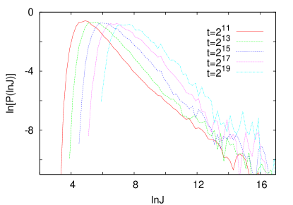
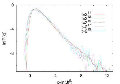
Figure 1: Left: Numerically calculated distribution of the logarithm of local currents at different times for the binary randomness with parameters $r=1/4$, $c=1/3$. The control parameter is $\mu=1/2$ and $\beta=1/2$. Right: Scaling plot of the same data.

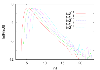
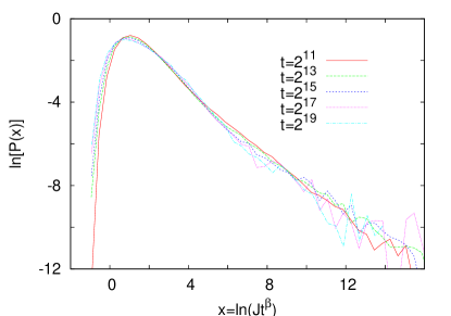
Figure 2: Left: Numerically calculated distribution of the logarithm of local currents at different times for the uniform randomness with $s=1.5$. The control parameter is $\mu\approx 0.37607$ and $\beta\approx 0.570734$. Right: Scaling plot of the same data.

As can be seen in the figures, an adequate data collapsing can be achieved using the scaling variable $Jt^{\beta}$ where $\beta$ is the exponent predicted by the theory in Eq. (45). The time-dependence of the typical current has been calculated in several points of the driven phase and the corresponding effective exponents $\beta_{\rm eff}(t)$ are plotted against time in Fig. 3. The obtained data are again in satisfactory agreement with the predictions of phenomenological theory.

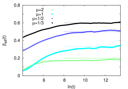
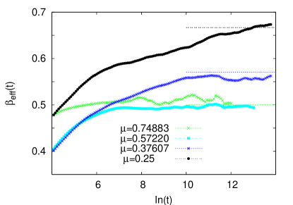
Figure 3: Effective exponent $\beta_{\rm eff}(t)$ plotted against time in different points of the driven phase. Left: Data are obtained with the binary randomness with parameters $c=0.2$, $r=0.5$ and $c=1/3$, $r=0.5,0.25,0.125$ where the control parameter is $\mu=2,1,1/2,1/3$, respectively. Right: Data are obtained with the uniform randomness with $s=3,2,1.5,1.29$ where $\mu\approx 0.7488,0.5722,0.3761,0.25$, respectively. The horizontal lines indicate the value of $\beta$ predicted the phenomenological theory.

The length $l(t)$ has been measured at the same points of the driven phase, as well. The corresponding effective exponents are compared to the predictions of phenomenological theory in Fig. 4. As can be seen, the finite time corrections are more considerable than those of $\beta$, nevertheless the asymptotic behavior is still compatible with the theory.

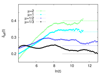
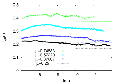
Figure 4: Effective exponent $\delta_{\rm eff}(t)$ plotted against time in different points of the driven phase. Left: Data are obtained with binary randomness with parameters $c=0.2$, $r=0.5$ and $c=1/3$, $r=0.5,0.25,0.125$ where the control parameter is $\mu=2,1,1/2,1/3$, respectively. Right: Data are obtained with the uniform randomness with $s=3,2,1.5,1.29$ where $\mu\approx 0.7488,0.5722,0.3761,0.25$, respectively. The horizontal lines indicate the value of $\delta$ predicted the phenomenological theory.

Next we turn to present numerical results obtained for zero average force ($\mu=0$). The distributions of local currents for different times are shown in Fig. 5 and 6. The striking difference compared to the driven phase is that, although the exponent $\beta$ is still finite ($\beta=1$) for $\mu=0$, the distributions are broadening with increasing time. A rough scaling collapse can be achieved in terms of the scaling variable $\ln(J)/\ln(t)$. Earlier results on the distribution of the stationary current in finite systems of size $L$ showed an approximate scaling collapse for the scaling variable $\ln(J)/L^{1/2}$ [15]. Taking into account the relation between time and length scale in Eq. (53), this is consistent with our present results on the dynamical scaling.

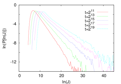
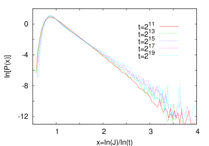
Figure 5: Left: Numerically calculated distribution of the logarithm of local currents at different times for the binary randomness with parameters $r=1/4$, $c=1/2$. At this point the average force is zero and $\mu=0$. Right: Scaling plot of the same data.

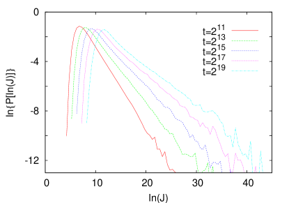
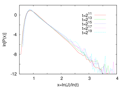
Figure 6: Left: Numerically calculated distribution of the logarithm of local currents at different times for uniform randomness with parameters $s=1$. At this point the average force is zero and $\mu=0$. Right: Scaling plot of the same data.

As can be seen in Fig. 7, the effective exponent $\beta_{\rm eff}(t)$ overshoots the expected asymptotical value $1$ by a few percent. This is in accordance with that the scaling collapse of distributions is not perfect and the shape of distributions is still slightly changing at the numerically available time scales. We have also measured the variance of local currents which enhances the contribution of large local currents compared to the typical value defined in Eq. (3). These lie just in the still deforming and thus poorly scaling part of distributions. The corresponding effective exponents are approaching the theoretical value from below, see Fig. 7.

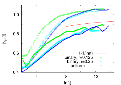
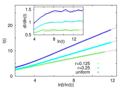
Figure 7: Left: The effective exponent $\beta_{\rm eff}(t)$ (open symbols) plotted against time for zero average force. Filled symbols show the effective exponents calculated from the variance of the current. The solid line corresponds to the form in Eq. (54). Right: Time-dependence of the length scale $l(t)$. The effective exponents are shown in the inset, where the solid lines corresponds to the form in Eq. (55).

In the right panel of Fig. 7, the measured length scale is plotted against time. As can be seen, the data are in good agreement with the law given in Eq. (55).

7 Discussion

The partially asymmetric simple exclusion process with random-force disorder has been investigated in earlier studies exclusively by Monte Carlo simulations and by a phenomenological random barrier description. In this work, a mean field approximation has been applied to this model and the main focus was on the non-stationary phenomena. The mean field approximation leads to a system of deterministic, nonlinear differential equations. This model is less complex than the original stochastic process but still not tractable analytically. Nevertheless, it is appropriate for applying a phenomenological random barrier theory to it. According to our analytical mean field calculations, the key issue of the theory, namely the current through a barrier has the same behavior as that has been assumed intuitively for the original model in earlier works. This leads to the same large-scale stationary and non-stationary behavior as has been conjectured for the original model. We have investigated the mean field model numerically, which is considerably faster than performing Monte Carlo simulations and have found that the dynamics is satisfactorily described by the phenomenological theory. Since a good agreement between the phenomenology and results of Monte Carlo simulations carried out on the original model has been found in earlier works, we conjecture that the mean field model belongs to the same universality class as the original stochastic process does. This means that the static and dynamical exponents in the driven phase, as well as the scaling relations for the case of zero average force are identical. Our results show that in the presence of disorder the local correlations are unimportant concerning the large scale behavior of the system. This conclusion can be instructive for the investigation of other transport processes with random-force disorder, where the simple mean field approximation may give the correct large scale behavior.

Appendix A

Let us denote the stationary local density in the pure model by $\rho$ and the deviation from the stationary density by $\epsilon_{i}(t)$, i.e. $\rho_{i}(t)=\epsilon_{i}(t)+\rho$. The spatially continuous limit of the evolution equations Eq. (1) reads as

$$\frac{\partial\epsilon}{\partial t}=D\frac{\partial^{2}\epsilon}{\partial x^{2}}-v\frac{\partial\epsilon}{\partial x}+\lambda\epsilon\frac{\partial\epsilon}{\partial x},$$ (61)

where the constants $D$, $v$ and $\lambda$ are given in terms of the jump rates as $D=(p+q)/2$, $v=(1-2\rho)(p-q)$ and $\lambda=2(p-q)$. The local current in the continuum limit takes the form

$$J(x,t)=J_{\infty}+v\epsilon-D\frac{\partial\epsilon}{\partial x}-\lambda\epsilon^{2},$$ (62)

where $J_{\infty}=(p-q)\rho(1-\rho)$ is the current in the steady state. First, let us consider the simplest case $p=q$, which describes the symmetric simple exclusion process. In this case, $v=\lambda=0$ and Eq. (61) reduces to the diffusion equation. Consider a random initial density profile of the form

$$\epsilon(x,0)=\sum_{n=-\infty}^{\infty}s_{n}\delta(x-n),$$ (63)

where $\delta(x)$ is the Dirac delta distribution and the $s_{n}$ are independent binary random variables with the probability density $f(s)=\frac{1}{2}\delta(s-1)+\frac{1}{2}\delta(s+1)$. The solution of Eq. (61) is then

$$\epsilon(x,t)=\frac{1}{\sqrt{4\pi Dt}}\sum_{n=-\infty}^{\infty}s_{n}\exp{\frac{-(x-n-vt)^{2}}{4Dt}}.$$ (64)

The mean value of local quantities such as the deviation $\overline{\epsilon(t)}=\lim_{L\to\infty}\frac{1}{2L+1}\sum_{n=-L}^{L}\epsilon(n,t)$ at time $t$ can be calculated alternatively from $\overline{\epsilon(t)}=\int\epsilon(0,t)f(s)ds$ since the $s_{n}$ are identically distributed for all $n$. For the mean deviation we obtain the obvious result $\overline{\epsilon(t)}=0$, since $\overline{\epsilon(0)}=0$ and the total mass $\int\rho(x,t)dx$ is conserved by Eq. (61). The fluctuations of $\epsilon(x,t)$ are characterized by the variance, the square of which can be easily calculated:

$$\overline{\epsilon^{2}(t)}=\frac{1}{4\pi Dt}\sum_{n=-\infty}^{\infty}\exp{\frac{-n^{2}}{2Dt}}\approx\frac{1}{4\pi Dt}\int_{-\infty}^{\infty}\exp{\frac{-x^{2}}{2Dt}}dx=(8\pi Dt)^{-1/2},$$ (65)

where the sum has been approximated by an integral. Thus, the typical deviation from the stationary density measured at a randomly chosen site at time $t$ is in the order of $t^{-1/4}$. The typical local current can be estimated in a similar way. The mean value $\overline{\frac{\partial\epsilon}{\partial x}}$ is zero while the square of the variance is

$$\overline{\left(\frac{\partial\epsilon}{\partial x}\right)^{2}}=\frac{1}{4\pi Dt}\sum_{n=-\infty}^{\infty}\frac{n^{2}}{4D^{2}t^{2}}\exp{\frac{-n^{2}}{2Dt}}\approx$$

$$\frac{1}{16\pi D^{3}t^{3}}\int_{-\infty}^{\infty}x^{2}\exp{\frac{-x^{2}}{2Dt}}dx=\frac{1}{16}\sqrt{\frac{2}{\pi}}(Dt)^{-3/2}.$$ (66)

The typical current measured at a given bond at time $t$ is thus $O(t^{-3/4})$.

In the case $p\neq q$, which corresponds to the asymmetric simple exclusion process, the Galilean transformation $x\to x+vt$ cancels the second term on the r.h.s. of Eq. (61) and one obtains the noiseless Burgers equation [19]:

$$\frac{\partial\epsilon}{\partial t}=D\frac{\partial^{2}\epsilon}{\partial x^{2}}+\lambda\epsilon\frac{\partial\epsilon}{\partial x}.$$ (67)

This can be exactly solved by the Cole-Hopf transformation (see e.g. [24]) $w(x,t)=\exp{\frac{\lambda}{2D}\int^{x}\epsilon(x^{\prime},t)dx^{\prime}}$, which maps the Burgers equation to the diffusion equation. The solution is obtained from

$$\epsilon(x,t)=\frac{2D}{\lambda}\frac{\partial\ln w}{\partial x},$$ (68)

with

$$w(x,t)=\int_{-\infty}^{\infty}\frac{1}{\sqrt{4\pi Dt}}\exp{\left(-\frac{(x-x^{\prime})^{2}}{4Dt}+\frac{\lambda}{2D}\int^{x^{\prime}}\epsilon(x^{\prime\prime},0)dx^{\prime\prime}\right)}dx^{\prime}.$$ (69)

Using the random initial condition given in Eq. (63), the deviation of the density at $x=0$ is given as

$$\epsilon(0,t)=\frac{1}{Dt}\frac{\int_{-\infty}^{\infty}x\exp{\left[-\frac{x^{2}}{4Dt}+\frac{\lambda}{2D}r(x)\right]}dx}{\int_{-\infty}^{\infty}\exp{\left[-\frac{x^{2}}{4Dt}+\frac{\lambda}{2D}r(x)\right]}dx},$$ (70)

where $r(x)=\int_{0}^{x}\epsilon(x^{\prime},0)dx^{\prime}$ is a piecewise constant function with unit jumps at integers whereas for non-integers it is given by $r(x)=-\frac{s_{0}}{2}+\sum_{n=0}^{[x]}s_{n}$, where $[x]$ denotes the integer part of $x$. Thus $r(x)$ can be regarded as a random walk which makes jumps at integer “times” $x$. It is easy to see that the mean value of the deviation $\overline{\epsilon(t)}$ is zero since $\overline{\exp{\frac{\lambda}{2D}r(x)}}$ is an even function of $x$ due to ${\rm Prob}[r(x)]={\rm Prob}[r(-x)]$. The typical value of the deviation at time $t$ can be obtained as follows. First notice that the r.h.s. of Eq. (70) can be regarded as the expected value of $x$ which has the (unnormalized) weight function $\exp{F(x)}$ with

$$F(x)=-\frac{x^{2}}{4Dt}+\frac{\lambda}{2D}r(x).$$ (71)

The dominant contribution to this expected value comes from the interval where $F(x)$ is maximal, since otherwise the weight $\exp{F(x)}$ is negligible. So we have the approximate relation $\epsilon(0,t)\sim\frac{1}{Dt}x_{\rm max}$, where $x_{\rm max}$ is the location of the maximum of $F(x)$. (In case there are many maxima, $x_{\rm max}$ is their mean value.) The distribution of $x_{\rm max}$ is symmetric around zero and the dependence of its magnitude on time can be obtained by taking into account that the variance of $r(x)$ which characterizes its typical magnitude is $\sqrt{\overline{r^{2}(x)}}=\sqrt{[x]+1/4}$, i.e. proportional to $\sqrt{x}$ for large $x$. Replacing $r(x)$ in Eq. (71) by $\sqrt{x}$, we obtain a non-random function the maximum of which is at $(2\lambda t)^{2/3}$. Thus the width of the distribution of $x_{\rm max}$ is in the order of $t^{2/3}$ and we obtain finally that the typical deviation from the stationary density measured at a given site scales with time as $\epsilon_{\rm typ}(t)\sim t^{-1/3}$. By a similar calculation one can show that the expected value of $\frac{\partial\epsilon}{\partial x}$ is of the order of $t^{2/3}$. Now we can turn to the analysis of the fluctuations of the current. If $\rho\neq 1/2$ then $v\neq 0$ and the fluctuations are dominated by the term $v\epsilon$, see Eq. (62). Thus the magnitude of the typical local current (relative to the stationary current) scales as $(J-J_{\infty})_{\rm typ}(t)\sim t^{-1/3}$. If, however, $\rho=1/2$, the above term is zero and the fluctuations are determined by the other two terms leading to $(J-J_{\infty})_{\rm typ}(t)\sim t^{-2/3}$.

References

References

- [1] J. Howard, Mechanics of Motor Proteins and the Cytoskeleton (Sinauer, Sunderland, 2001) Schliwa M and Woehlke G, 2003 Nature 422 759 Gross S P, 2004 Phys. Biol. 1 R1 Chowdhury D, Schadschneider A, Nishinari K 2005 Physics of Life Reviews (Elsevier, New York) vol. 2, p. 318
- [2] MacDonald C T, Gibbs J H and Pipkin A C, 1968 Biopolymers 6 1
- [3] Spitzer F, 1970 Adv. Math. 5 246
- [4] Liggett T M 1999 Stochastic interacting systems: contact, voter, and exclusion processes (Berlin, Springer)
- [5] Schmittmann B and Zia R K P 1995 in Phase Transitions and Critical Phenomena, vol. 17, edited by Domb C and Lebowitz J L (Academic, London)
- [6] Schütz G M 2001 in Phase Transitions and Critical Phenomena, vol. 19, edited by Domb C and Lebowitz J L (Academic, San Diego)
- [7] Blythe R A, Evans M R 2007 J. Phys. A Math. Theor. 40 R333
- [8] Ramaswamy R, Barma M 1987 J. Phys. A: Math. Gen. 20 2973
- [9] Koscielny-Bunde E, Bunde A, Havlin S, and Stanley H E, 1988 Phys. Rev. A 37 1821
- [10] Tripathy G, Barma M 1997 Phys. Rev. Lett. 78 3039; 1998 Phys. Rev. E 58 1911
- [11] Goldstein S, Speer E R 1998 Phys. Rev. E 58 4226
- [12] Kolwankar K M, Punnoose A 2000 Phys. Rev. E 61 2453
- [13] Krug J, 2000 Braz. J. Phys. 30 97
- [14] Harris R J, Stinchcombe R B 2004 Phys. Rev. E 70 016108
- [15] Juhász R, Santen L and Iglói F, 2005 Phys. Rev. Lett. 94 010601; 2006 Phys. Rev. E 74 061101
- [16] Juhász R, Lin Y-C, Iglói F 2006 Phys. Rev. B 73 224206
- [17] Barma M, 2006 Physica A 372 22
- [18] Greulich P, Schadschneider A 2008 J. Stat. Mech. P04009
- [19] Burgers J M 1974 The Nonlinear Diffusion Equation (Riedel, Boston)
- [20] Blythe R A, Evans M R, Colaiori F, Essler F H L 2000 J. Phys. A: Math. Gen. 33 2313
- [21] Iglói F, Rieger H 1998 Phys. Rev. E 58 4238
- [22] For a review see: Bouchaud J P, Georges A 1990 Phys. Rep. 195 127
- [23] Press W H, Teukolsky S A, Wetterling W T, Flannery B P 1992 Numerical Recipes in C (Cambridge University Press, Cambridge)
- [24] Stinchcombe R B 2001 Adv. in Phys. 50 431