Theoretical description of three- and four-nucleon scattering states using bound-state-like wave functions

Abstract

Bound-state-like wave functions are used to determine the scattering matrix corresponding to low energy $N-d$ and $p-^{3}$He collisions. To this end, the coupled channel form of the integral relations derived from the Kohn variational principle is used. The construction of degenerate bound-state-like wave functions belonging to the continuum spectrum of the Hamiltonian is discussed. Examples are shown using realistic nucleon-nucleon forces.

I Introduction

Well established methods to treat both, bound and scattering states in $A=3,4$ systems, are the solution of the Faddeev ($A=3$) or Faddeev-Yakubovsky ($A=4$) equations in configuration or momentum space and the hyperspherical harmonic (HH) expansion in conjunction with the Kohn variational principle (KVP). These methods have proven to be of great accuracy and they have been tested through different benchmarks benchmark1 ; benchmark2 . On the other hand, other methods are presently used to describe bound states: for example, the Green’s Function Monte Carlo (GFMC) and No Core Shell Model (NCSM) methods have been used in nuclei up to $A=10$ and $A=12$ respectively gfmc ; ncsm . Attempts to use these methods in the description of scattering states recently appeared gfmc5 ; ncsm5 .

The possibility of employing bound state techniques to describe scattering states has always attracted particular attention harris . Recently, continuum-discretized states obtained from the stochastic variational method have been used to study single channel $\alpha+n$ scattering scattering suzuki1 . The extension to treat coupled channel scattering is given in Ref. suzuki2 . In those approaches, the tangent of the phase-shift results in a quotient of two numbers. In the former the numerator and denominator are obtained from two integral relations after projecting the Schrödinger equation, whereas in the latter the numerator results from an integral relation derived by means of the Green’s function formalism and the denominator from the normalization of the continuum-discretized state.

Recently two integral relations have been derived from the KVP intrel . It has been shown that starting from the KVP, the tangent of the phase-shift can be expressed as a quotient where both, the numerator and the denominator, are given as two integral relations. This is similar to what was proposed in Ref. harris , however the variational character of the quotient and its strict relation with the KVP were not recognized. In fact, it is this characteristic that makes possible many different and interesting applications of the integral relations. For example, in Ref. kiev10a , the integral relations have been used to compute phase-shifts from bound state like functions in the $A=2,3$ systems using semirealistic interactions. Both $n-d$ and $p-d$ scattering were considered. The latter process is of particular interest since $p-d$ scattering at low energies has been a subject of intense investigations. Initially, the Faddeev method has been applied mainly to the neutral $n-d$ reaction. Applications to $p-d$ zero-energy scattering were studied in configuration space by the Los Alamos-Iowa group using $s$-wave potentials friar83 and realistic forces friar84 . In those calculations the KVP was used to correct the first order estimate of the scattering length after solving the Faddeev equations in which the partial wave expansion of the Coulomb potential was truncated. Low-energy $p-d$ elastic scattering has been studied using the pair correlated hyperspherical harmonic (PHH) expansion phh ; kiev01a as well. A benchmark between these two techniques was given in Ref. kiev01b . A different way to treat the Coulomb potential in few-nucleon scattering was proposed in Ref. deltuva1 , based on the works of Ref. alt , in which the Alt-Grassberger-Sandhas equations were solved using a screened Coulomb potential and then the scattering amplitude was obtained after a renormalization procedure. A benchmark for elastic $p-d$ scattering up to $65$ MeV between this technique and the PHH expansion using the KVP has been performed benchmark3 .

Summarizing, the description of scattering states using very accurate methods are at present circumscribed to $A\leq 4$ systems. On the other hand, accurate methods to describe bound states beyond the $A=4$ mass system exist. Therefore the discussion of new methods to extend these approaches to treat scattering states is of interest. In this discussion the treatment of the Coulomb interaction cannot be neglected. In the present work we would like to show a detailed application of the integral relations derived from the KVP in which $A=3,4$ bound-state-like wave functions are used to compute the scattering matrix using realistic nucleon-nucleon $NN$ potentials. In particular, we face the problem of constructing degenerate bound state wave functions at a given energy $E$ belonging to the continuum spectrum of the Hamiltonian. In fact, in the $A=3$ system, the elastic scattering matrix is a $2\times 2$ matrix for $J^{\pi}=1/2^{\pm}$ and a $3\times 3$ matrix for all the other states. This means that, at energies below the deuteron breakup threshold, there are two (for $J^{\pi}=1/2^{\pm}$) or three (for $J>1/2$) scattering states, at the same energy, differing in their asymptotic structure. For example, in the $J^{\pi}=1/2^{+}$ state, two different asymptotic structures exist corresponding to $(L,S)=(0,1/2)$ or $(2,3/2)$, being $L$ the relative angular momentum between the deuteron and the incoming nucleon and $S$ the total spin $S$. Therefore, at a given energy, the two scattering states have a particular combination of the two different asymptotic structures determined by the scattering matrix. In the present paper we discuss how to construct degenerate bound-state wave functions at a particular energy, belonging to the continuum spectrum of the Hamiltonian. Moreover, these states will be used in the integral relations to compute the scattering matrix. Examples using realistic forces in the $A=3,4$ systems will be shown. We expect that this study will serve as a guide for calculating scattering states in systems with $A>4$.

The paper is organized as follow. In the next section general $A=3,4$ bound-state wave functions are constructed using the HH expansion. In Section III, a brief derivation of the KVP given in terms of the integral relations is discussed. Applications to the $A=3,4$ systems are shown in Section IV whereas the conclusions are given in the last section.

II $A=3,4$ bound like states with arbitrary $J^{\pi}$ values

Following Refs. phh ; kiev93 ; kiev97 ; report we give a brief description of a general three- and four- nucleon bound state in terms of the hyperspherical harmonic basis. In the case of $A=3$, a bound-state wave function can be written as a sum of three amplitudes

$$\Psi=\psi({\bf x}_{i},{\bf y}_{i})+\psi({\bf x}_{j},{\bf y}_{j})+\psi({\bf x}_{k},{\bf y}_{k})\ ,$$ (1)

where ${\bf x}_{i},{\bf y}_{i}$ are the internal Jacobi coordinates which are defined in terms of the particle coordinates as

$${\bf x}_{i}={\bf r}_{j}-{\bf r}_{k}\,,\quad{\bf y}_{i}={1\over{\sqrt{3}}}({\bf r}_{j}+{\bf r}_{k}-2{\bf r}_{i})\ .$$ (2)

Each $i$–amplitude has total angular momentum and parity $J^{\pi}$ and third component of the total isospin $T_{z}$. Using $LS$ coupling, it can be decomposed into channels

$$\psi({\bf x}_{i},{\bf y}_{i}) = \sum_{\alpha}^{N_{c}}\phi_{\alpha}(x_{i},y_{i}){\cal Y}_{\alpha}(jk,i)$$ (3)

$${\cal Y}_{\alpha}(jk,i) = \Bigl{\{}\bigl{[}Y_{\ell_{\alpha}}(\hat{\bf x}_{i})Y_{L_{\alpha}}(\hat{\bf y}_{i})\bigr{]}_{\Lambda_{\alpha}}\bigl{[}s_{\alpha}^{jk}s_{\alpha}^{i}\bigr{]}_{S_{\alpha}}\Bigr{\}}_{JJ_{z}}\;\bigl{[}t_{\alpha}^{jk}t_{\alpha}^{i}\bigr{]}_{T_{\alpha}T_{z}},$$ (4)

where $x_{i},y_{i}$ are the moduli of the Jacobi coordinates. Each $\alpha$–channel is labeled by the angular momenta $\ell_{\alpha},L_{\alpha}$, coupled to $\Lambda_{\alpha}$, and by the spin (isospin) $s_{\alpha}^{jk}$ ($t_{\alpha}^{jk}$) of the pair $j,k$, coupled to the spin (isospin) of the third particle $s_{\alpha}^{i}$ ($t_{\alpha}^{i}$) to give $S_{\alpha}$ ($T_{\alpha}$). $N_{c}$ is the number of channels taken into account in the construction of the wave function and should be increased until convergence is reached. The antisymmetrization of the state requires that $\ell_{\alpha}+s_{\alpha}^{jk}+t_{\alpha}^{jk}$ be odd, while the parity of the state is given by $\ell_{\alpha}+L_{\alpha}$.

Defining the hyperradius and hyperangle in terms of the moduli of the Jacobi coordinates

$$x_{i}=\rho\cos\phi_{i}\,,\,\,\,\,\,\,\,y_{i}=\rho\sin\phi_{i}$$ (5)

the two–dimensional spatial amplitudes can be expanded in terms of the PHH basis as

$$\phi_{\alpha}(x_{i},y_{i})=\rho^{\ell_{\alpha}+L_{\alpha}}f_{\alpha}(x_{i})\left[\sum_{K}u^{\alpha}_{K}(\rho){}^{(2)}P^{\ell_{\alpha},L_{\alpha}}_{K}(\phi_{i})\right]\ ,$$ (6)

where the hyperspherical polynomials are

$${}^{(2)}P^{\ell_{\alpha},L_{\alpha}}_{K}(\phi_{i})=N_{n}^{\ell_{\alpha},L_{\alpha}}(\sin\phi_{i})^{L_{\alpha}}(\cos\phi_{i})^{\ell_{\alpha}}P_{n}^{L_{\alpha}+1/2,\ell_{\alpha}+1/2}(\cos 2\phi_{i})\ .$$ (7)

$N_{n}^{\ell_{\alpha},L_{\alpha}}$ is a normalization factor, $P_{n}^{\alpha,\beta}$ is a Jacobi polynomial and $K=\ell_{\alpha}+L_{\alpha}+2n$ is the grand orbital quantum number which runs from its minimum value $K_{0}=\ell_{\alpha}+L_{\alpha}$ to its maximum selected value $K_{\alpha}$. Therefore, the number of hyperradial functions per channel is $M_{\alpha}=(K_{\alpha}-K_{0})/2+1$. The inclusion of the pair correlation function $f_{\alpha}(x_{i})$ in the expansion of Eq.(6) accelerates the convergence taking into account the correlations introduced by the strong repulsion of the $NN$ potential (see for example Ref.kiev93 ).

In the case of the four-nucleon system we use the HH expansion as described in Ref. viv05 . The wave function having total angular momentum $J$ and parity $\pi$ can be cast in the form

$$\Psi=\sum_{[K]}\sum_{\alpha}u^{\alpha}_{[K]}(\rho)\Psi_{\alpha}^{[K]}\ ,$$ (8)

where $[K]\equiv K,\Lambda,S,T$ and $\Psi_{\alpha}^{[K]}$ are the channel HH-spin-isospin functions having grand angular momentum $K$, orbital angular momentum $\Lambda$, coupled to total spin $S$, to give a total angular momentum $JJ_{z}$, and total isospin $T$. The channel index $\alpha$ labels the possible choices of hyperangular, spin and isospin quantum numbers, namely

$$\alpha\equiv\{\ell_{1},\ell_{2},\ell_{3},L_{2},n_{2},n_{3},S_{a},S_{b},T_{a},T_{b}\}\ ,$$ (9)

compatibles with the given values of $K$, $\Lambda$, $S$, $T$, $J$ and $\pi$. The channel function $\Psi_{\alpha}^{[K]}$ is constructed as a linear combination of the following basis elements

$$\Psi^{[K]}_{\alpha}=\biggl{\{}{\cal Y}^{K,\Lambda,M}_{\ell_{1},\ell_{2},\ell_{3},L_{2},n_{2},n_{3}}(\Omega)\biggl{[}\Bigl{[}\bigl{[}s_{1}s_{2}\bigr{]}_{S_{a}}s_{3}\Bigr{]}_{S_{b}}s_{4}\biggr{]}_{SS_{z}}\biggr{\}}_{JJ_{z}}\biggl{[}\Bigl{[}\bigl{[}t_{1}t_{2}\bigr{]}_{T_{a}}t_{3}\Bigr{]}_{T_{b}}t_{4}\biggr{]}_{TT_{z}}\ .$$ (10)

Here, ${\cal Y}^{K,\Lambda,M}_{\ell_{1},\ell_{2},\ell_{3},L_{2},n_{2},n_{3}}(\Omega)$ is the four-nucleon HH state and $s_{i}$ ($t_{i}$) denotes the spin (isospin) function of particle $i$ and $\Omega$ indicates the set of the four-nucleon hyperangular variables. The total parity of the state is given by $\pi=(-1)^{\ell_{1}+\ell_{2}+\ell_{3}}$.

In the present work the $A=3,4$ hyperradial functions $u^{\alpha}_{[K]}(\rho)$ are taken as linear combinations of Laguerre polynomials multiplied by an exponential function:

$$u^{\alpha}_{[K]}(\rho)=\sum_{m}A_{\alpha,[K],m}L^{(\gamma)}_{m}(z)\exp(-z/2)\ ,$$ (11)

where $A_{\alpha,[K],m}$ are coefficients to be determined and the indeces $\alpha,[K]$ label either a three-nucleon or a four-nucleon channel. The polynomials depend on the variable $z=\beta\rho$, with $\beta$ a nonlinear variational parameter. Let us define $|\alpha,[K],m>$ as a totally antisymmetric element of the expansion basis for the $A=3,4$ systems. In terms of the basis elements, the bound-state wave functions given in Eqs.(1) and (8) can be written as

$$\Psi_{n}=\sum_{\alpha,[K],m}A^{n}_{\alpha,[K],m}|\alpha,[K],m>.$$ (12)

The index $n$ indicates the level of the state with energy $E_{n}$. The linear coefficients $A^{n}_{\alpha,[K],m}$ of the wave function and the energy of the state are obtained by solving the following generalized eigenvalue problem

$$\sum_{\alpha^{\prime},[K^{\prime}],m^{\prime}}A^{n}_{\alpha^{\prime},[K^{\prime}],m^{\prime}}<\alpha,[K],m|H-E_{n}|\alpha^{\prime},[K^{\prime}],m^{\prime}>=0\ .$$ (13)

In the latter equation the dimension of the involved matrices is related to three indices: the number of $\alpha$–channels $N_{c}$, the number of hyperspherical polynomials for each channel $M_{\alpha}$ and, $N_{L}$ the number of Laguerre polynomials included in the expansion of the hyperradial functions of Eq.(11). The convergence properties of the expansion is analyzed by increasing the indices $K,m$ and studying the stability obtained for different values of the nonlinear parameter $\beta$. The ground state of the three-nucleon system has total angular momentum and parity $J^{\pi}=1/2^{+}$ and with $N_{c}=18$ an accuracy of $1$ keV is reached kiev97 ; kame89 . The corresponding dimension of the PHH basis is $D\approx 2200$, considering $M_{\alpha}=8$ for the first $8$ channels, $M_{\alpha}=6$ for the successive six channels, $M_{\alpha}=4$ in the last ones and including $N_{L}\approx 20$ Laguerre polynomials in the description of the hyperradial functions. After the diagonalization of the whole matrix, $D$ eigenvalues are obtained. The lowest one corresponds to the three-nucleon ground state and, with the very extended basis used, it shows a noticeable stability with $\beta$. A certain number of negative eigenvalues verifying $E_{n}>E_{d}$ (with $E_{d}$ the deuteron energy) also appear. Defining the positive energy $E^{0}_{n}=E_{n}-E_{d}$, the corresponding eigenvectors $\Psi_{n}$ approximately describe a scattering process at the center-of-mass energy $E^{0}_{n}$, though asymptotically they go to zero. The eigenvalues $E_{n}$ present a monotonic behavior with $\beta$, as shown in the left panel of Fig. 1, where the AV14 $NN$ potential av14 has been used.

In the right panel of Fig. 1 the lowest eigenvalues obtained from a diagonalization of the $J^{\pi}={1/2^{-}}$ state are shown. As expected this state is not bound, though several negative states appear with energies in the interval $E_{d}<E_{n}<0$, characterized with a monotonic behavior with $\beta$. As before, these states approximately describe a scattering process at the center-of-mass energy $E^{0}_{n}$. In Fig. 1 the deuteron energy is indicated by the dotted-dashed line whereas the three dashed lines indicate the lab energies $E_{lab}=1,2,3$ MeV, respectively. Interestingly, the energies of the $J^{\pi}=1/2^{-}$ state appear in pairs. This can be understood noticing that the $J^{\pi}=1/2^{-}$ scattering states are twofold degenerate at a given energy, as the scattering matrix has dimension of two. This degeneration arises from the two possible asymptotic configurations in which the relative angular momentum of the deuteron and the third nucleon is $L=1$ and the total spin can take the values $S=1/2$ and $3/2$. Also the $J^{\pi}=1/2^{+}$ state is twofold degenerate, having two possible asymptotic configuration with the values $L=0,S=1/2$ and $L=2,S=3/2$. However, in this case, the different $L$ values produce different contributions to the kinetic energy with the consequence that the two degenerate states appears with a larger separation compared to the $J^{\pi}=1/2^{-}$ case. However, this difference reduces as the basis is enlarged.

To analyze further the hypotesis that the states organize in pairs corresponding to the two different asymptotic configurations in both $J^{\pi}=1/2^{\pm}$ states, in Table 1 the different occupation probabilities are given. For the $J^{\pi}=1/2^{+}$ state the occupation probabilities of the $S$- $P$ and $D$-waves, $P_{S},P_{P}$ and $P_{D}$, have been computed. The $E_{0}$ level corresponds to the ground state and the successive levels organize in mostly $S$-wave ($E_{1}$ and $E_{3}$) and mostly $D$-wave ($E_{2}$ and $E_{4}$) states, alternatively. In the case of the $J^{\pi}=1/2^{-}$ state, the occupation probabilities of the $P$-wave with total spin values $S=1/2$ and $3/2$, $P^{1/2}_{P}$ and $P^{3/2}_{P}$, as well as $P_{D}$ have been computed. From the table we can observe that the levels organize in pairs, being one of the states mostly a $P$-wave state with $S=1/2$ and the other mostly a $P$-wave state with $S=3/2$. This organization is indicated in Fig. 1 with colors. For the $J^{\pi}=1/2^{+}$ the $E_{0}$ level, shown as a black solid line, is practically constant with $\beta$. The levels with high $L=0$ ($L=2$) occupation probability are given in red (blue) respectively. In the case of the $J^{\pi}=1/2^{-}$, the levels with high $P_{P}^{3/2}$ ($P_{P}^{1/2}$) probabilities are given in red (blue) respectively. For small values of $\beta$ the spectrum tends to be denser since, in this case, the polynomials can contain more oscillations before the action of the exponential tail becomes significant. As $\beta$ increases the number of negative eigenvalues decreases. In the case in which a bound state exists, as in the case of the $J^{\pi}=1/2^{+}$ state, the basis is sufficiently large to guarantee a correct description of it as the control parameter $\beta$ is varied. As we will see, the wave functions $\Psi_{n}$ corresponding to energy levels $E_{d}<E_{n}<0$, can be used to determine the scattering matrix at specific energies.

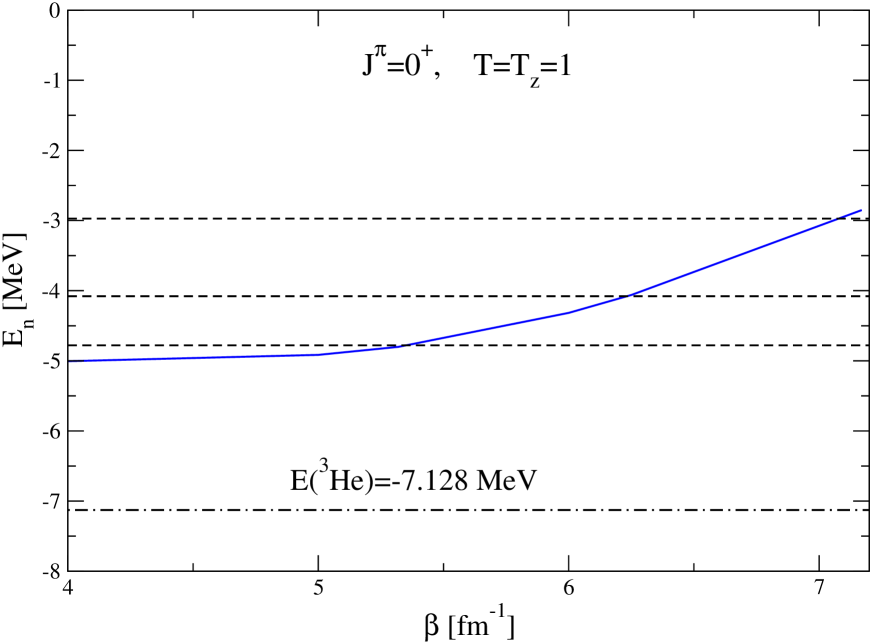
Figure 2: (Color online) The lowest $A=4$ eigenvalue, using the N3LO potential, for the $J^{\pi}=0^{+}$ state with $T=T_{z}=1$ as a function of the nonlinear parameter $\beta$. The colored lines indicate the eigenvalues embedded in the continuum as explained in the text. The dotted-dashed line represents the triton energy, the dashed lines indicate the labs energies $E_{lab}=3.13,4.05,5.54$ MeV.

In the case of the $A=4$ system we analyze the single channel $J^{\pi}=0^{+}$ state with $T=T_{z}=1$, corresponding to the $p-^{3}{\rm He}$ system. Using the N3LO-Idaho potential N3LO , the Hamiltonian matrix has a total dimension $D\approx 84000$, obtained expanding the wave function on the HH basis, as as previously described, with $K_{max}=44$, corresponding to about $3500$ HH states, and $N_{L}=24$. For this values of $D$, the matrix can be diagonalized using standard iterative methods. In Fig. 2 the first eigenvalue is shown as a function of the control parameter $\beta$. Clearly the lowest eigenvalue is above the ³He threshold, fixed for the N3LO-Idaho potential at -7.128 MeV, since four nucleons in the isospin channel $T=1$ does not present a bound state. The three dashed lines correspond to three lab energies (3.13, 4.05 and 5.54 MeV) at which experimental data exist. Similar to the previous cases in $A=3$, we will use these four-body bound state wave functions to determine the $p-^{3}{\rm He}$ scattering matrix at the indicated energies.

III The KVP in terms of integral relations

Following Refs. kiev01a ; report a general scattering state with $A=3,4$ can be written as a sum of two terms

$$\Psi=\Psi_{C}+\Psi_{A}\ .$$ (14)

The first term, $\Psi_{C}$, describes the system when the $A$ nucleons are close to each other. For large interparticle separations and energies below the breakup threshold in more than two pieces it goes to zero, whereas for higher energies it must reproduce a three or four outgoing particle state. It can be written as a sum of amplitudes corresponding to the cyclic permutations of the Jacobi coordinates. Each amplitude $\Psi_{C}(\{{\bf x}_{i}\})$ has total angular momentum and parity $J^{\pi}$ and third component of the total isospin $T_{z}$ (here $\{{\bf x}_{i}\}$ represents the set of Jacobi coordinates with ordering of the particles $i$ for the $A=3$ or $A=4$ systems). For energies below the breakup threshold in three pieces, it can be expanded in terms of the totally antisymmetric states

$$\Psi_{C}=\sum_{\alpha,[K],m}A_{\alpha,[K],m}|\alpha,[K],m>.$$ (15)

The second term, $\Psi_{A}$, in the scattering wave function of Eq.(14) describes the relative motion of the two clusters in the asymptotic region. For $A=3$, $\Psi_{A}$ describes the relative motion between the deuteron and the incident nucleon, whereas for $A=4$ we will limited the description to an incident nucleon on ³He or ³H. It can be written as a sum of amplitudes whose generic form for $A=3$ is given by

$$\Omega^{\lambda}_{LSJ}({\bf x}_{i},{\bf y}_{i})=\sum_{l_{\alpha}=0,2}w_{l_{\alpha}}(x_{i}){\cal R}^{\lambda}_{L}(y_{i})\left\{\left[[Y_{l_{\alpha}}({\hat{x}}_{i})s_{\alpha}^{jk}]_{1}s^{i}\right]_{S}Y_{L}({\hat{y}}_{i})\right\}_{JJ_{z}}[t_{\alpha}^{jk}t^{i}]_{TT_{z}}\ ,$$ (16)

where $w_{l_{\alpha}}(x_{i})$ is the $l_{\alpha}=0,2$ deuteron wave function, $s_{\alpha}^{jk}=1,t_{\alpha}^{jk}=0$, and $L$ is the relative angular momentum of the deuteron and the incident nucleon. The superscript $\lambda$ indicates the regular ($\lambda\equiv R$) or the irregular ($\lambda\equiv I$) solution of the Schrödinger equation in the asymptotic region. In the $p-d$ ($n-d$) case, the functions ${\cal R}^{\lambda}$ are related to the regular or irregular Coulomb (spherical Bessel) functions. The functions $\Omega^{\lambda}$ can be combined to form a general asymptotic state

$$\Omega^{+}_{LSJ}=\sum_{i=1,3}\left[\Omega^{0}_{LSJ}({\bf x}_{i},{\bf y}_{i})+\sum_{L^{\prime}S^{\prime}}{}^{J}{\cal L}^{SS^{\prime}}_{LL^{\prime}}\Omega^{1}_{L^{\prime}S^{\prime}J}({\bf x}_{i},{\bf y}_{i})\right]\ ,$$ (17)

where

$$\Omega^{0}_{LSJ}({\bf x}_{i},{\bf y}_{i})= u_{00}\Omega^{R}_{LSJ}({\bf x}_{i},{\bf y}_{i})+u_{01}\Omega^{I}_{LSJ}({\bf x}_{i},{\bf y}_{i})\ ,$$ (18)

$$\Omega^{1}_{LSJ}({\bf x}_{i},{\bf y}_{i})= u_{10}\Omega^{R}_{LSJ}({\bf x}_{i},{\bf y}_{i})+u_{11}\Omega^{I}_{LSJ}({\bf x}_{i},{\bf y}_{i})\ .$$ (19)

The matrix elements $u_{ij}$ form a matrix $u$ that can be selected according to the four different choices of the matrix ${\cal L}=$ ${\cal K}$-matrix, ${\cal K}^{-1}$-matrix, $S$-matrix or $T$-matrix. It should be noticed that the irregular solution has been opportunely regularized at the origin

$${\cal R}^{I}_{L}(y)=(1-{\rm e}^{-\gamma r_{Nd}})^{L+1}G_{L}(y)$$ (20)

where $r_{Nd}=(\sqrt{3}/2)\;y$ is the nucleon-deuteron separation and the parameter $\gamma$ is fixed requiring that ${\cal R}^{I}_{L}(y)\equiv G_{L}(y)$ asymptotically. Moreover, $G_{L}(y)$ is the irregular Bessel function or the irregular Coulomb function in the case of $n-d$ or $p-d$ scattering, respectively. The description for $A=4$ can be found in Ref. fisher06

A general three- or four-nucleon scattering wave function for an incident state with relative orbital angular momentum $L$, spin $S$, total angular momentum $J$ and energy below the three-particle breakup threshold is

$$|\Psi^{+}_{LSJ}>=\sum_{\alpha,[K],m}A^{LSJ}_{\alpha,[K],m}|\alpha,[K],m>+|\Omega^{+}_{LSJ}>\ ,$$ (21)

and its complex conjugate is $\Psi^{-}_{LSJ}$. A variational estimate of the trial parameters in the wave function $\Psi^{+}_{LSJ}$ can be obtained by requiring, in accordance with the generalized KVP, that the functional

$$[{}^{J}{\cal L}^{SS^{\prime}}_{LL^{\prime}}]={}^{J}{\cal L}^{SS^{\prime}}_{LL^{\prime}}-{2\over{\rm det}(u)}\langle\Psi^{-}_{LSJ}|H-E|\Psi^{+}_{L^{\prime}S^{\prime}J}\rangle\ ,$$ (22)

be stationary. Applications of the complex KVP for $N-d$ scattering can be found for example in Refs. kiev97 ; kiev01a ; marcucci09 . In the case in which the variational principle is formulated in terms of the ${\cal K}$-matrix, we get:

$$[{}^{J}{\cal K}^{SS^{\prime}}_{LL^{\prime}}]={}^{J}{\cal K}^{SS^{\prime}}_{LL^{\prime}}-\langle\Psi^{-}_{LSJ}|H-E|\Psi^{+}_{L^{\prime}S^{\prime}J}\rangle\ .$$ (23)

Calling the set of indeces $\mu\{\equiv\alpha,[K],m\}$ and $i=\{L,S,J\}$, the variation of the functional $[\;{}^{J}{\cal K}^{SS}_{LL}]\equiv[\;{\cal K}_{ii}]$ with respect to the linear parameters $A^{i}_{\mu}$ leads to the following two sets of linear equations

$$\sum_{\mu^{\prime}}<\mu|H-E|\mu^{\prime}>A^{0,i}_{\mu^{\prime}}=-<\mu|H-E|\Omega^{0}_{i}>$$ (24)

$$\sum_{\mu^{\prime}}<\mu|H-E|\mu^{\prime}>A^{1,i}_{\mu^{\prime}}=-<\mu|H-E|\Omega^{1}_{i}>\ ,$$ (25)

in accordance of the two possible asymptotic scattering states $\Omega^{0}_{i}$ and $\Omega^{1}_{i}$. From the above equations the two sets of coefficients $A^{0,i}_{\mu},A^{1,i}_{\mu}$ can be obtained. Furthermore, multiplying the sets by these coefficients and summing on $\mu$, it is possible to reconstruct the scattering state and the above equations can be formally cast as

$$<\Psi_{C}|H-E|\Psi^{+}_{i}>=0\,.$$ (26)

The variation of the functional with respect to the linear parameters ${\cal K}_{ij}$ results

$$\delta_{ij}-<\Omega^{1}_{j}|H-E|\Psi^{+}_{i}>-<\Psi^{-}_{i}|H-E|\Omega^{1}_{j}>=0\,.$$ (27)

Using the normalization condition

$$<\Omega^{0}_{i}|H-E|\Omega^{1}_{j}>-<\Omega^{1}_{j}|H-E|\Omega^{0}_{i}>=\delta_{ij}\;,$$ (28)

the scattering wave function verifies

$$<\Psi^{-}_{i}|H-E|\Omega^{1}_{j}>-<\Omega^{1}_{j}|H-E|\Psi^{+}_{i}>=\delta_{ij}$$ (29)

$$<\Omega^{0}_{i}|H-E|\Psi^{+}_{j}>-<\Psi^{-}_{j}|H-E|\Omega^{0}_{i}>={\cal K}_{ij}\;,$$ (30)

allowing to reduce Eq.(27) to

$$<\Omega^{1}_{j}|H-E|\Psi^{+}_{i}>=0\,.$$ (31)

The second order estimates of the ${\cal K}$-matrix elements $[\;^{J}{\cal K}^{SS^{\prime}}_{LL^{\prime}}]\equiv[\;{\cal K}_{ii^{\prime}}]$ are obtained replacing in the functional of Eq.(23), the first order solutions given by Eqs.(26) and (31). It results

$$[\;{\cal K}_{ii^{\prime}}]=\;{\cal K}_{ii^{\prime}}-<\Omega^{0}_{i}|H-E|\Psi^{+}_{i^{\prime}}>$$ (32)

that can be further reduced using Eq.(30) to

$$[\;{\cal K}_{ii^{\prime}}]=-<\Psi^{-}_{i}|H-E|\Omega^{0}_{i^{\prime}}>\;.$$ (33)

This final form of the KVP is a direct consequence of the particular form selected for the asymptotic scattering state given in Eq.(17) in which the flux of the regular wave $\Omega^{0}_{i}$ has been set to one. As we will see in the following, it is useful to define an asymptotic scattering state with general coefficients in both the regular and irregular waves. Accordingly, the asymptotic scattering state now reads

$$\Omega^{+}_{LSJ}=\sum_{i=1,3}\left[\sum_{L^{\prime}S^{\prime}}{}^{J}\!\!{\cal A}^{SS^{\prime}}_{LL^{\prime}}\,\Omega^{0}_{L^{\prime}S^{\prime}J}({\bf x}_{i},{\bf y}_{i})+\sum_{L^{\prime}S^{\prime}}{}^{J}{\cal B}^{SS^{\prime}}_{LL^{\prime}}\,\Omega^{1}_{L^{\prime}S^{\prime}J}({\bf x}_{i},{\bf y}_{i})\right]\ .$$ (34)

The coefficients ${}^{J}\!\!{\cal A}^{SS^{\prime}}_{LL^{\prime}}$ and ${}^{J}{\cal B}^{SS^{\prime}}_{LL^{\prime}}$ form the matrices ${\cal A}$ and ${\cal B}$ respectively and the scattering matrix results ${\cal K}={\cal A}^{-1}{\cal B}$. Starting with a scattering state that has this asymptotic behavior, the relations of Eqs.(29) and (30) result

$$<\Psi^{-}_{i}|H-E|\Omega^{1}_{j}>-<\Omega^{1}_{j}|H-E|\Psi^{+}_{i}>={\cal A}_{ij}$$ (35)

$$<\Omega^{0}_{i}|H-E|\Psi^{+}_{j}>-<\Psi^{-}_{j}|H-E|\Omega^{0}_{i}>={\cal B}_{ij}\;,$$ (36)

and, using Eqs.(31)-(33), the KVP takes the particular form

$${\cal A}_{ij} = <\Psi^{-}_{i}|H-E|\Omega^{1}_{j}>$$ (37)

$$[{\cal B}_{ij}] = -<\Psi^{-}_{i}|H-E|\Omega^{0}_{j}>$$ (38)

$$[{\cal K}] = {\cal A}^{-1}[{\cal B}]$$ (39)

where $[{\cal B}]$ and $[{\cal K}]$ are second order estimates.

Eqs.(39) formulate the KVP in terms of integral relations depending on the internal structure of the scattering wave function $\Psi^{-}_{i}$. In fact $(H-E)\Omega^{0}_{j}$ and $(H-E)\Omega^{1}_{j}$ go to zero as each of the three Jacobi coordinates $y_{k}$ goes to $\infty$ $(k=1,2,3)$, since $\Omega^{0,1}_{j}$ are the solutions of $(H-E)$ in that limit. Therefore, in Eqs.(39), it would be possible to use trial wave functions $\Psi^{-}_{i}$ that are solutions of $(H-E)$ in the interaction region but do not have the physical asymptotic behavior indicated in Eq.(34). In particular, it would be possible to use the bound-state wave functions $\Psi_{n}$ described in the previous section to calculate the scattering matrix corresponding to a center-of-mass energy $E^{0}_{n}$. This is discussed in the next section.

IV Scattering matrix from bound-state-like wave functions

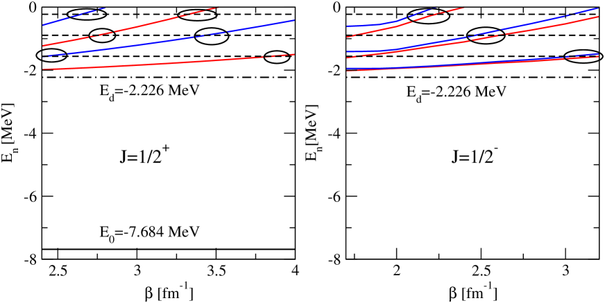
Figure 3: (Color online) The same as Fig.1 in which two sequential solutions having the same eigenvalue are selected (indicated by the circles) in the three cases corresponding to incident energies $E_{lab}=1,2,3$ MeV respectively.

In section II the construction of $A=3,4$ bound states having general quantum numbers $J^{\pi}$ corresponding to different levels with negative eigenvalues $E_{n}$ has been discussed. In the case of the $A=3$ state $J=1/2^{+}$ the $E_{0}$ level and the corresponding wave function $\Psi_{0}$ describe the energy and structure of the triton or ³He for the two possible values of $T_{z}=1/2$ or $-1/2$, respectively. Using the nonlinear parameter $\beta$ as a control parameter it was possible to construct states with eigenvalues $E_{n}$ in the region $E_{d}<E_{n}<0$. In a similar way, it is possible to contruct these kind of states for arbiratry values of $J^{\pi}$. As an example, in section II, the case $J=1/2^{-}$ was explicitly discussed. Furthermore, it was shown that these states organize sequentially having occupation probabilities that can be connected with the different components of a scattering state, corresponding to the different values of the quantum numbers $L,S,J$. The number of these components fixes the dimension of the scattering matrix and, correspondingly, the degeneration of the state. Therefore, in order to construct a scattering state using bound-state-like functions, those components can be taken into account considering sequential solutions having the same energy. To this end the control parameter $\beta$ can be used to select sequential solutions at the same eigenvalue $E_{n}$. This is shown in Fig. 3 for three different cases. The three dashed lines in both panels of the figure indicate the energies corresponding to incident energies in the lab system $E_{lab}=1,2,3$ MeV. As explained in section II, the red and blue lines show the variation of sequential eigenvalues as a function of $\beta$ having the different structures given in Table 1. The circles in Fig. 3 indicate the points in wich the eigenvalues cross the dashed lines and, accordingly, at those specific values of $\beta$ two different solutions, $\Psi^{1}_{n}$ and $\Psi^{2}_{n}$, can be constructed having the same energy $E_{n}$ and presenting a very different internal structure. These two states are solutions of $(H-E_{n})\Psi^{1,2}_{n}=0$ in the internal region and, since they are square integrable states, they go to zero asymptotically. However the integral relations of Eq.(39) depend on the internal part of the wave function and therefore it would be possible to use $\Psi^{1}_{n}$ and $\Psi^{2}_{n}$ as trial wave functions. In this case the second order estimate of the scattering matrix is

$${\cal A}_{ij} = <\Psi^{i}_{n}|H-E_{n}|\Omega^{1}_{j}>$$ (40)

$$[{\cal B}_{ij}] = -<\Psi^{i}_{n}|H-E_{n}|\Omega^{0}_{j}>$$ (41)

$$[{\cal K}] = {\cal A}^{-1}[{\cal B}]$$ (42)

where $i,j$ indicate either the two solutions, $\Psi^{1,2}_{n}$, and the two possible values of the set of quantum numbers $(L,S,J)$ in $J=1/2^{\pm}$.

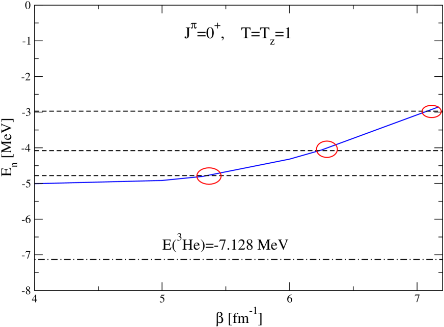
Figure 4: (Color online) The same as Fig.2 in which the lowest eigenvalue is selected (indicated by the circles) in the three cases corresponding to the lab energies $E_{cm}=3.13,4.05,5.54$ MeV respectively.

For the $A=4$ case we have analyzed the single channel $J^{\pi}=0^{+}$ state with $T=T_{z}=1$. In Fig. 4 we show the three cases (indicated with circles) at which, for specific values of the control parameter $\beta$, the eigenvalue matches the selected energies. Accordingly the second order estimate of the scattering matrix can be obtained in each case as

$${\cal A} = <\Psi_{n}|H-E_{n}|\Omega^{1}>$$ (43)

$$[{\cal B}] = -<\Psi_{n}|H-E_{n}|\Omega^{0}>$$ (44)

$$[{\cal K}] = {\cal A}^{-1}[{\cal B}]$$ (45)

In this case we are considering a single channel state and therefore the scattering matrix results a scalar.

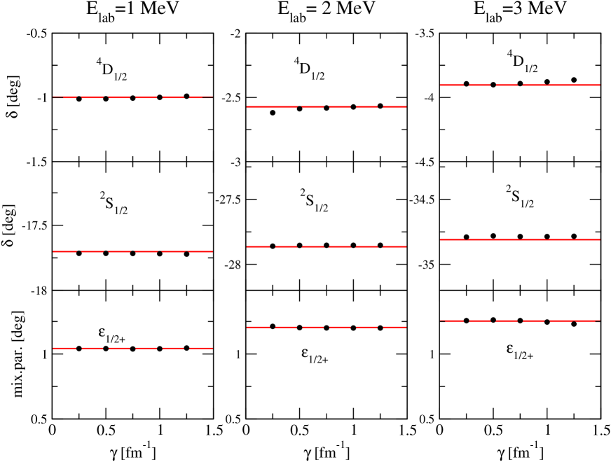
Figure 5: (Color online) The $n-d$ $J^{\pi}=1/2^{+}$ phase-shifts and mixing parameters as a function of the regularization parameter $\gamma$ at the three indicated energies. The red line corresponds to the results of Ref. benchmark1 .

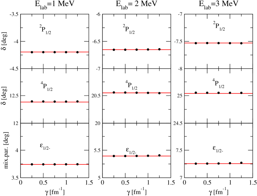
Figure 6: (Color online) The $n-d$ $J=1/2^{-}$ phase-shifts and mixing parameters, for the AV14 potential, as a function of the regularization parameter $\gamma$ at the three indicated energies. The red line corresponds to the results of Ref. benchmark1 .

In the following, results of phase-shifts and mixing parameters for the $n-d$ system, calculated using the AV14 $NN$ potential, are presented for the $J^{\pi}=1/2^{+}$ state in Fig. 5, and for the $J^{\pi}=1/2^{-}$ state in Fig. 6, at the three selected energies $E_{lab}=1,2,3$ MeV. The stability of the results with $\gamma$, the regularization parameter introduced in Eq.(20), is chosen as a convergence criterion. This criterion has been discussed in Refs. intrel ; kiev10a and essentially it establishes the quality of $\Psi_{n}^{i}$ as solution of $(H-E_{n})\Psi_{n}^{i}=0$. In fact, if $\Psi_{n}^{i}$ is a good solution, the integrals of Eq.(42) are largely independent of $\gamma$. The results are compared to the benchmark of Ref. benchmark1 given in the figures as a red line. The results of the application of Eq.(42) are shown as filled circles corresponding to values of $\gamma$ varying from $0.25$ fm^-1 to $1.25$ fm^-1. We can observed a good stability on this interval and, furthermore, the results are in very good agreement with those of Ref benchmark1 .

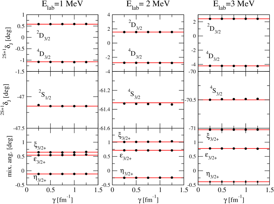
Figure 7: (Color online) The $n-d$ $J=3/2^{+}$ phase-shifts and mixing parameters, for the AV14 potential, as a function of the regularization parameter $\gamma$ at the three indicated energies. The red line corresponds to the results of Ref. benchmark1 .

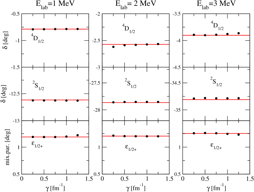
Figure 8: (Color online) The $p-d$ $J=1/2^{+}$ phase-shifts and mixing parameters, for the AV14 potential, as a function of the regularization parameter $\gamma$ at the three indicated energies. The red line corresponds to the results of Ref. kiev01b .

In Fig. 7 results are given for the $n-d$ $J^{\pi}=3/2^{+}$ state. In this case the ${\cal K}$-matrix is a $3\times 3$ matrix, corresponding to asymptotic configurations having $L=0,S=3/2$, $L=2,S=1/2$ and $L=2,S=3/2$. The diagonalization of the Hamiltonian matrix in the $J^{\pi}=3/2^{+}$ case produces sequential eigenvalues with occupation probabilities in accordance with these three configuration. Using the control parameter $\beta$, three sequential eigenvalues can be chosen to have a particular $E_{n}$ value as has been done before for the $J^{\pi}=1/2^{\pm}$ states. In the figure we observe a good stability with the regularization parameter $\gamma$ and a close agreement with the results of the Ref. benchmark1 . In Fig. 8 results for the $p-d$ $J=1/2^{+}$ state are given. The description of the $p-d$ process at low energies presents some problems using the Faddeev equations. In Ref. kiev01b a benchmark for $p-d$ scattering has been produced using the HH method and the Faddeev method in configuration space. The results of the benchmark are shown as a red line in Fig. 8. From the figure we can observe that the results using the integral relations reproduce extremely well the benchmark results. This is an important point since in bound-state-type calculations the treatment of the Coulomb potential does not present any troubles.

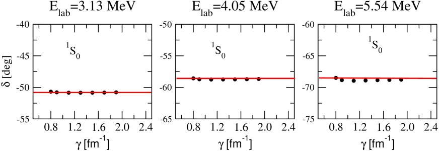
Figure 9: (Color online) The $p-^{3}\!{\rm He}$ $J=0^{+}$ phase-shift, for the N3LO potential, as a function of the regularization parameter $\gamma$ at the three indicated energies. The red line corresponds to the results of Ref. benchmark4b .

The $p-^{3}{\rm He}$ results are given in Fig. 9 for the three selected energies. The phase-shift for the $0^{+}$ state is shown as a function of the regularization parameter $\gamma$ (filled circles). As a comparison, the results of the recent benchmark of Ref. benchmark4b are shown as a red line. We can observe a good stability with $\gamma$ indicating that the four-nucleon bound-state eigenfunction $\Psi$ is a good solution of $(H-E)\Psi=0$ at the specified energies. Moreover the results obtained using the integral relations are in close agreement with those of the benchmark.

V Conclusions

In this work the elastic scattering matrix has been determined using bound-state-like wave functions. To this end two integral relations derived from the KVP have been used. Initially, these integral relations were derived in Ref. intrel in order to extract phase shifts from the solutions calculated using the hyperspherical adiabatic expansion in the three-nucleon system. In this method the boundary conditions at large distances are imposed in terms of the hyperradius $\rho$. However, as explained in Ref. intrel , the boundary conditions depend explicitly on the Jacobi coordinates ${\bf x}_{i},{\bf y}_{i}$ describing the asymptotic configuration of a deuteron formed by particles $(j,k)$ and an incoming nucleon (particle $i$). The equivalence between imposing the boundary conditions in $\rho$ or in the Jacobi coordinates directly, results at very large values of the hyperradius where the relation $\rho\approx y_{i}$ is verified. As a consequence, the phase shifts obtained from the adiabatic expansion require a large number of terms to converge. On the other hand, the phase shifts obtained as a quotient of the two integral relations converge much faster and, in fact, the rate of convergence is similar to that one obtained in the case of bound state solutions. The reason behind this fact is that the integral relations depend only on the internal part of the wave function. Therefore, it is enough that the wave function verifies $(H-E)\Psi=0$ in the internal region to obtain almost exact results for the scattering matrix at the center-of-mass energy $E$. This characteristic allows to apply the integral relations using bound-state-like wave functions obtained from a direct diagonalization of the Hamiltonian $H$. Eigenvectors corresponding to eigenvalues belonging to the continuum spectrum of $H$ can be used as inputs to determine the scattering matrix at fixed values of $E$. Applications for single-channel solutions using semi-realistic $NN$ potentials are given in Ref. kiev10a . The coupled-channel case of an atom colliding a dimer formed by other two atoms is given in Ref. romero10 .

In the present work, applications to elastic scattering of a nucleon on a deuteron ($A=3$) or on ³He ($A=4$) below the breakup threshold, using realistic nucleon-nucleon potentials has been discussed. In particular, for $A=3$, two or three solutions at the same energy have to be determined corresponding to the different possible asymptotic configurations of the system. A detailed construction of such solutions, using the nonlinear parameter $\beta$ as a control parameter, has been analyzed. Moreover it has been shown that the eigenvectors of successive eigenvalues organize in pairs (for $J=1/2^{\pm}$) or in triplets (for $J>1/2$), corresponding to the different asymptotic structures. The control parameter $\beta$ has been tuned to find solutions having the same eigenvalue that have been usend to calculate the scattering matrix at the selected energy. The obtained results are in close agreement with those presented in the $A=3$ benchmarks of Refs. benchmark1 ; kiev01b and in the $A=4$ benchmark of Ref.benchmark4b . In particular, the results for $p-d$ and $p-^{3}{\rm He}$ scattering demonstrate that the scattering matrix can be calculated using bound-state-like wave functions also in scattering of charged particles.

Well established bound-state methods to diagonalize the nuclear Hamiltonian in systems with $A>4$ already exist. The formulation of the scattering matrix presented in this work will allow to extent these studies to the low-energy continuum spectrum. It will be then possible to compare theoretical predictions for scattering observables to the experimental data, in order to evaluate the capability of the present models for the interaction to describe the nuclear structure. Studies along this line are at present intensively pursued.

$J=1/2^{+}$	$P_{S}(\%)$	$P_{P}(\%)$	$P_{D}(\%)$
$E_{0}$	90.96	0.08	8.97
$E_{1}$	90.04	0.00	5.96
$E_{2}$	1.22	2.72	96.06
$E_{3}$	94.20	0.00	5.80
$E_{4}$	1.21	2.70	96.09
$J=1/2^{-}$	$P^{1/2}_{P}(\%)$	$P^{3/2}_{P}(\%)$	$P_{D}(\%)$
$E_{1}$	3.36	94.87	1.77
$E_{2}$	93.80	3.42	2.78
$E_{3}$	3.47	94.71	1.82
$E_{4}$	93.42	3.86	2.72
$E_{5}$	4.32	93.87	2.01
$E_{6}$	92.72	4.77	2.51

Table 1: Occupation probabilities of the different states shown in Fig. 1 at $\beta=2.5$ fm^-1 ($J^{\pi}=1/2^{+}$) and $\beta=2.0$ fm^-1 ($J^{\pi}=1/2^{-}$).

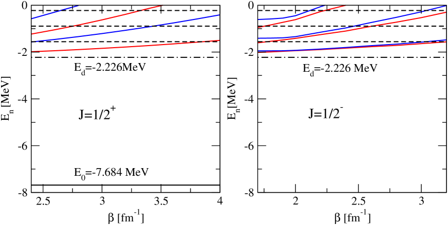
Figure 1: (Color online) The lowest $A=3$ eigenvalues, using the AV14 potential, for the $J^{\pi}=1/2^{+}$ (left panel) and $J^{\pi}=1/2^{-}$ (right panel) states, as a function of the nonlinear parameter $\beta$. The solid black line (left panel) represents the triton energy whereas the colored lines indicate the eigenvalues embedded in the continuum as explained in the text. The dotted-dashed line represents the deuteron energy, the dashed lines indicate the labs energies $E_{lab}=1,2,3$ MeV.

References

- (1) A. Kievsky et al., Phys. Rev. C58, 3085 (1998)
- (2) R. Lazauskas, J. Carbonell, A.C. Fonseca, M. Viviani, A. Kievsky, and S. Rosati, Phys. Rev. C71, 034004 (2005)
- (3) S.C. Pieper, K. Varga, and R.B. Wiringa, Phys. Rev. C66, 044310 (2002)
- (4) P. Navrátil, V.G. Gueorguiev, J.P. Vary, W.E. Ormand, and A. Nogga, Phys. Rev. Lett. 99, 042501 (2007)
- (5) K.M. Nollett, S.C. Pieper, R.B. Wiringa, J. Carlson, and G.M. Hale, Phys. Rev. Lett. 99, 022502 (2007)
- (6) S. Quaglioni and P. Navrátil, Phys. Rev. C79, 044606 (2009)
- (7) F.E. Harris, Phys. Rev. Lett. 19, 173 (1967)
- (8) Y. Suzuki, W. Horiuchi, and K. Arai, Nucl. Phys. A823, 1 (2009)
- (9) Y. Suzuki, M. Baye, and A. Kievsky, Nucl. Phys. A838, 20 (2010)
- (10) P. Barletta, C. Romero-Redondo, A. Kievsky, M. Viviani, and E. Garrido, Phys. Rev. Lett. 103, 090402 (2009)
- (11) A. Kievsky, M. Viviani, P. Barletta, C. Romero-Redondo, and E. Garrido, Phys. Rev. C81, 034002 (2010)
- (12) J.L. Friar, B.F. Gibson, and G.L. Payne, Phys. Rev. C28, 983 (1983)
- (13) J.L. Friar, B.F. Gibson, G.L. Payne, and C.R. Chen, Phys. Rev. C30, 1121 (1984)
- (14) A. Kievsky, M. Viviani, and S. Rosati, Nucl. Phys. A577, 511 (1994)
- (15) A. Kievsky, M. Viviani, and S. Rosati, Phys. Rev. C64, 024002 (2001)
- (16) A. Kievsky, J.L. Friar, G.L. Payne, S. Rosati, and M. Viviani, Phys. Rev. C63, 064004 (2001)
- (17) A. Deltuva, A.C. Fonseca, and P.U. Sauer, Phys. Rev. C71, 054005 (2005)
- (18) E.O. Alt, W. Sandhas, and H. Ziegelmann, Phys. Rev. C17, 1981 (1978); E.O. Alt and W. Sandhas, Phys. Rev. C21, 1733 (1980)
- (19) A. Deltuva, A.C. Fonseca, A. Kievsky, S. Rosati, P.U. Sauer, and M. Viviani, Phys. Rev. C71, 064003 (2005)
- (20) A. Kievsky, M. Viviani, and S. Rosati, Nucl. Phys. A551, 241 (1993)
- (21) M. Viviani, A. Kievsky, and S. Rosati, Phys. Rev.C71, 024006 (2005)
- (22) A. Kievsky, Nucl. Phys. A624, 125 (1997)
- (23) A. Kievsky, S. Rosati, M. Viviani, L.E. Marcucci, and L. Girlanda, J. Phys. G: Nucl. Part. Phys. 35 063101 (2008)
- (24) H. Kameyama, M. Kamimura, and Y. Fukushima, Phys. Rev. C40, 974 (1989)
- (25) R. B. Wiringa, R. A. Smith, and T. L. Ainsworth, Phys. Rev. C29, 1207 (1984)
- (26) D.R. Entem and R. Machleidt, Phys. Rev C68, 041001 (2003)
- (27) B.M. Fisher et al., Phys. Rev C74, 034001 (2006)
- (28) L.E. Marcucci, A. Kievsky, L. Girlanda, S. Rosati and M. Viviani, Phys. Rev C80, 034003 (2009)
- (29) M. Viviani, A. Deltuva, R. Lazauskas, J. Carbonell, A.C. Fonseca, A. Kievsky, L.E. Marcucci, and S. Rosati, arXiv:1109.3625, submitted to Phys. Rev. C
- (30) C. Romero-Redondo, E. Garrido, P. Barletta, A. Kievsky, and M. Viviani, Phy. Rev. A83, 022705 (2011)