Theory of robust subrecoil cooling by STIRAP

Abstract

We demonstrate one-dimensional robust Raman cooling in a three-level $\Lambda$-type atom, where the velocity-selective transfer is carried out by a STIRAP pulse. In contrast to the standard Raman method, the excitation profile is insensitive to variations in the pulse duration, whereas its position and width are nevertheless under control. Two different cooling variants are examined and we show that subrecoil temperatures are attainable in both cases.

I Introduction

The physics of cold atoms is an important ingredient in the emerging field of quantum technology, either providing elements for demanding applications or a transparent testing ground for ideas and methods Mabuchi2002 ; Bloch2008a ; Bloch2008b . This is made possible by sophisticated control of both translational and internal degrees of freedom for neutral atoms with electromagnetic fields, demonstrated especially by laser cooling and trapping methods Metcalf1999 ; Weidemuller2009 ; Cohen-Tannoudji2011 . One of the most notable successes has been the reaching of quantum degeneracy, i.e., Bose-Einstein condensation with bosonic atoms, and Cooper pairing with fermionic atoms Weidemuller2009 ; Cohen-Tannoudji2011 ; Pethick2008 . Here the key tools have been evaporative cooling and magnetic trapping, as reaching the ultralow temperatures and high densities with laser light is usually hampered by heating and loss of atoms due to light-assisted atomic collisions Holland1994 ; Suominen1996 or reabsorption of scattered photons Steane1992 ; Cooper1994 .

Evaporative cooling, however, is rather wasteful of atoms and requires fast thermalizing collisions, which limits its practicality in some cases, such as single-species fermionic gases Duarte2011 ; MacKay2011 , atomic clocks Ye2008 ; Derevianko2011 , or small samples of cold atoms Phoonthong2010 , and especially transversal cooling of atomic beams Theuer1999 ; Vewinger2003 . Very recently, for instance, fermionic atoms have been efficiently laser cooled using narrow optical transitions, which lead to low Doppler temperatures Duarte2011 ; MacKay2011 . The same approach has been used earlier with alkaline-earth atoms, for the purpose of building atomic clocks for optical wavelengths Ye2008 ; Derevianko2011 . In general, state-insensitive traps are needed for quantum state engineering and precision metrology Ye2008 ; Phoonthong2010 ; Derevianko2011 . Similarly, one needs to develop alternatives also for evaporative cooling. A simple possibility is to develop further the concept of Raman cooling; one of the aspects that can be improved is the robustness in respect to the laser pulse parameters. One of the success stories in robust quantum control of internal state dynamics is the use of adiabatic following of eigenstates, i.e., stimulated rapid adiabatic passage (STIRAP) Vitanov2001 . As known e.g. with molecular dynamics Garraway1998 ; Rodriguez2000 , it can also be used to control motional degrees of freedom.

Raman cooling Kasevich1992 is one the most efficient non-evaporative techniques for optical cooling of atoms below the one-photon recoil limit. The cooling efficiency is associated with population transfer which is typically generated by a $\pi$-pulse that has a Blackman Kasevich1992 ; Davidson1994 ; Reichel1994 or a square Reichel1995 ; Boyer2004 envelope. Although such a $\pi$-pulse operates efficiently on atoms corresponding to the resonant velocity group, the process requires extreme control of the pulse amplitude and duration. Even though some optimization can be obtained for the method Ivanov2011 , an approach based on adiabatic passage is of definite interest due to its robustness regarding pulse amplitudes and durations. However, the use of adiabatic passage in Raman cooling is not possible without having an exact understanding of its velocity-selective properties. In this paper we present a careful analysis of the Raman cooling via STIRAP pulses, and show that subrecoil temperatures are attainable.

The possibility to use adiabatic passage for optical cooling was demonstrated by Korsunsky Korsunsky1996 , being applied to VSCPT Aspect1988 cooling. Raman cooling is a much greater challenge which requires a careful analysis of the velocity selection process. Another difficulty consists in a reasonable choice of adiabatic passage which would demonstrate a benefit from its usage in Raman cooling. For instance, Raman cooling employing rapid adiabatic passage (RAP) was presented in papers Kuhn1996 ; Perrin1998 ; Perrin1999 , where the amplitude and the frequency of Raman pulses are changed in a controlled way, producing a velocity-selective transfer of the atomic population. The extent of the frequency-chirp determines the range of excitation by RAP and makes it possible to transfer even the wing of the velocity distribution. However, RAP does not give an appreciable advantage over ordinary Raman cooling, because the excitation profile depends on the amount of chirping, the pulse area and its envelope. The theory presented in this paper shows that the utilization of stimulated Raman adiabatic passage (STIRAP) Gaubatz1990 ; Bergmann1998 in contrast leads to a crucial growth of cooling robustness. In fact, once the adiabaticity criterion is fulfilled, the velocity selection in a case of large upper-level detuning depends only on the pulse amplitudes, allowing wide variations in the pulse duration.

This paper is organized as follows. After describing the basic atom-pulse setup in Sec. II, we discuss the adiabaticity criterion in Sec. III. Assuming that this criterion is satisfied, we present in Sec. IV the conditions of the adiabatic conversion for internal atomic states required for cooling. In Sec. V we discuss the velocity selection process and in Sec. VI the elementary cooling cycle. As the full cooling process requires a series of these cycles, and the adiabaticity criterion should be fulfilled for each cycle, we formulate in Sec. VII two possible approaches: a) using STIRAP pulses of equal amplitude, but with durations and amplitudes that vary during the pulse cycle series (in analogy with the standard Raman method, see e.g. Ref. Ivanov2011 ), and b) using STIRAP pulses of substantially different amplitudes, but not changing their duration and amplitude during the pulse cycle series. In the latter case, the amplitudes are adjusted to transfer the wing of the velocity distribution together with the possibility to cool the atomic ensemble below the recoil limit. The cooling results for a series of cycles for these two different transfer types are presented and discussed. The paper is concluded by the summary given in Sec. VIII.

II The atomic Hamiltonian

Figure 1(a) illustrates a three-level $\Lambda$-type atom that travels along direction $Oz$ with velocity $v$, being originally prepared in ground state $|1\rangle$. A pump laser propagating along the $Oz$ axis couples the atomic transition $|1\rangle\leftrightarrow|2\rangle$, whereas the contra-propagating Stokes laser couples the transition $|2\rangle\leftrightarrow|3\rangle$. The electric field of laser pulses is written as

$$\mathbf{E}(\mathbf{r},t)=\frac{1}{2}\mathbf{E}_{P}e^{ikz-i\omega_{P}t}+\frac{1}{2}\mathbf{E}_{S}e^{-ikz-i\omega_{S}t}+\text{c.c.},$$

where $\omega_{P}$, $\omega_{S}$ are the corresponding laser frequencies, and $k$ is the wave number for both light beams (the relevant frequency quantities are in fact the atom-field detunings, which are small compared to the actual frequencies, and thus we can assume equal values of $k$). The pump and Stokes pulses produce a velocity-selective STIRAP from the $|1\rangle$ to $|3\rangle$ ground state.

(a) (b)

Figure 1: (a) A three-level $\Lambda$-type atom interacting with a pair of contra-propagating laser beams. The pump laser links the initial state $|1\rangle$ with an intermediate state $|2\rangle$, whereas the Stokes laser links the intermediate state with the final state $|3\rangle$. (b) Both the pump and Stokes pulse have a Gaussian profile in time, overlapping during period $\Delta\tau$.

The total Hamiltonian for the atom-light system consists of the kinetic-energy term $\hat{\mathbf{P}}^{2}/2M$, the Hamiltonian of the $\Lambda$-type atom and the interaction Hamiltonian $\hat{V}$:

$$\hat{H}=\frac{\hat{\mathbf{P}}^{2}}{2M}+\sum_{j}E_{j}|j\rangle\langle j|+\hat{V}.$$

The laser-atom coupling $\hat{V}$ is the sum of couplings with both the pump and Stokes pulse, and in the rotating-wave approximation (RWA) is given by

$$\hat{V}_{P}=-\frac{d_{21}E_{P}}{2}|2\rangle\langle 1|e^{ikz-i\omega_{P}t}\\ -\frac{d_{23}E_{S}}{2}|2\rangle\langle 3|e^{-ikz-i\omega_{S}t}+\mbox{H.c.},$$

where $d_{21}$, $d_{23}$ are the corresponding electric dipole moments; H.c. is the Hermitian conjugate. The Rabi frequencies

$$\Omega_{P}=-\frac{d_{21}E_{P}}{\hbar},\quad\Omega_{S}=-\frac{d_{23}E_{S}}{\hbar}$$

are considered to be real-valued and positive, and thus the coupling $\hat{V}$ is written as

$$\hat{V}=\frac{\hbar\Omega_{P}}{2}|2\rangle\langle 1|e^{ikz-i\omega_{P}t}+\frac{\hbar\Omega_{S}}{2}|2\rangle\langle 3|e^{-ikz-i\omega_{S}t}+\mbox{H.c.}$$ (1)

Considering $z$ in Eq. (1) as an operator acting on the external degrees of freedom of the atom, we apply in Eq. (1) the relationship

$$e^{\pm ikz}=\sum_{p}|p\rangle\langle p\mp\hbar k|.$$

The obtained laser-atom coupling

$$\hat{V}=\sum_{p}\left(\frac{\hbar\Omega_{P}}{2}|2,p\rangle\langle 1,p-\hbar k|e^{-i\omega_{P}t}\right.\\ \left.\vphantom{\frac{1}{2}}+\frac{\hbar\Omega_{S}}{2}|2,p\rangle\langle 3,p+\hbar k|e^{-i\omega_{S}t}\right)+\text{H.c.}$$ (2)

shows that three states coupled by the pump and Stokes pulses form a momentum family

$$\mathcal{F}(p)=\{|1,p-\hbar k\rangle,|2,p\rangle,|3,p+\hbar k\rangle\}.$$

As long as spontaneous emission is not taken into account, a single family $\mathcal{F}(p)$ of a specific momentum $p$ can be only taken into account, so the sum in Eq. (2) is avoided.

In the basis of the three states

$$|a_{1}\rangle =\exp\left[-i\left(\frac{E_{1}}{\hbar}+\frac{(p-\hbar k)^{2}}{2M\hbar}\right)t\right]|1,p-\hbar k\rangle,$$

$$|a_{2}\rangle =\exp\left[-i\left(\frac{E_{2}}{\hbar}+\frac{(p-\hbar k)^{2}}{2M\hbar}+\Delta_{P}\right)t\right]|2,p\rangle,$$

$$|a_{3}\rangle =\exp\left[-i\left(\frac{E_{3}}{\hbar}+\frac{(p-\hbar k)^{2}}{2M\hbar}+\Delta_{P}-\Delta_{S}\right)t\right]|3,p+\hbar k\rangle,$$

the dynamics of an atom starting from state $|a_{1}\rangle$ with the corresponding velocity $v=(p-\hbar k)/M$ is described by the atomic Hamiltonian

$$\tilde{H}=\hbar\begin{bmatrix}0&\dfrac{1}{2}\Omega_{P}(t)&0\\ \dfrac{1}{2}\Omega_{P}(t)&\dfrac{kp}{M}-\omega_{R}-\Delta_{P}&\dfrac{1}{2}\Omega_{S}(t)\\ 0&\dfrac{1}{2}\Omega_{S}(t)&\dfrac{2kp}{M}+\Delta_{S}-\Delta_{P}\end{bmatrix},$$ (3)

where $\Delta_{P}=\omega_{P}-\omega_{21}$, $\Delta_{S}=\omega_{S}-\omega_{23}$ are the pulse detunings; $\omega_{R}=\hbar k^{2}/2M$ is the recoil frequency.

The pump and Stokes pulses evolve in time as Gaussian profiles shown in Fig. 1(b), being arranged in the counterintuitive sequence with $t_{S}<t_{P}$:

$$\Omega_{P}(t)=\Omega_{P0}e^{-(t-t_{P})^{2}/2T_{P}^{2}},\quad\Omega_{S}(t)=\Omega_{S0}e^{-(t-t_{S})^{2}/2T_{S}^{2}},$$

where $2T_{P}$, $2T_{S}$ are pulse widths. These lasers stimulate a velocity-selective STIRAP from the $|a_{1}\rangle$ state to the $|a_{3}\rangle$ state. The corresponding resonant velocity group is considered in Sec. III, whereas Sec. IV and Sec. V are devoted to an arbitrary velocity group in the case of large enough detunings $\Delta_{P}$ and $\Delta_{S}$.

III Two-photon resonance

Two-photon resonance is characterized by momentum $p=M(\Delta_{P}-\Delta_{S})/2k$, for which the detuning from state $|3\rangle$ in representation (3) equals zero. Thus an atom prepared in state $|1\rangle$ falls into the resonance, if it starts with resonant velocity

$$v_{0}=\frac{\Delta_{P}-\Delta_{S}}{2k}-v_{\mathrm{rec}},$$ (4)

where $v_{\mathrm{rec}}$ is the recoil velocity. Under this condition, the basis of time-dependent eigenstates of the Hamiltonian (3) is given by (see Ref. Bergmann1998 )

$$\begin{aligned} &|a^{+}\rangle=\sin\Theta\sin\Phi|a_{1}\rangle+\cos\Phi|a_{2}\rangle+\cos\Theta\sin\Phi|a_{3}\rangle,\\ &|a^{0}\rangle=\cos\Theta|a_{1}\rangle-\sin\Theta|a_{3}\rangle,\\ &|a^{-}\rangle=\sin\Theta\cos\Phi|a_{1}\rangle-\sin\Phi|a_{2}\rangle+\cos\Theta\cos\Phi|a_{3}\rangle.\end{aligned}$$ (5)

The corresponding (time-dependent) dressed-state eigenvalues are

$$\begin{aligned} \omega^{+}&=\frac{1}{2}\left(\sqrt{\tilde{\Delta}_{P}^{2}+\Omega_{P}^{2}(t)+\Omega_{S}^{2}(t)}-\tilde{\Delta}_{P}\right),\quad\omega^{0}=0,\\ \omega^{-}&=\frac{1}{2}\left(\sqrt{\tilde{\Delta}_{P}^{2}+\Omega_{P}^{2}(t)+\Omega_{S}^{2}(t)}+\tilde{\Delta}_{P}\right),\end{aligned}$$

where $\tilde{\Delta}_{P}=\Delta_{P}+\omega_{R}-kp/M$. The angle $\Phi$ is a function of the Rabi frequencies and detunings Fewell1997 :

$$\tan\Phi=\frac{\sqrt{\Omega_{P}^{2}(t)+\Omega_{S}^{2}(t)}}{\sqrt{\tilde{\Delta}_{P}^{2}+\Omega_{P}^{2}(t)+\Omega_{S}^{2}(t)}-\tilde{\Delta}_{P}},$$ (6)

whereas the mixing angle $\Theta$ depends only on Rabi frequencies:

$$\tan\Theta=\frac{\Omega_{P}(t)}{\Omega_{S}(t)}.$$ (7)

In the case of large detuning $\Delta_{P}$ ($\Omega_{P}(t),\Omega_{S}(t)\ll|\Delta_{P}|$), the basis of eigenstates $\{|a^{+}\rangle,|a^{0}\rangle,|a^{-}\rangle\}$ is reduced to the basis of states $\{|\mathrm{C}\rangle,|\mathrm{NC}\rangle,|a_{2}\rangle\}$. Both the coupled $|\mathrm{C}\rangle$ and non-coupled $|\mathrm{NC}\rangle$ state is a combination of ground states:

$$\begin{aligned} &|\mathrm{C}\rangle=\sin\Theta|a_{1}\rangle+\cos\Theta|a_{3}\rangle,\\ &|\mathrm{NC}\rangle=\cos\Theta|a_{1}\rangle-\sin\Theta|a_{3}\rangle,\end{aligned}$$ (8)

with the corresponding eigenvalues

$$\omega_{\mathrm{C}}=\frac{\Omega_{P}^{2}(t)+\Omega_{S}^{2}(t)}{4\Delta_{P}},\quad\omega_{\mathrm{NC}}=0.$$

Here, we take into account that $|\Delta_{P}|\gg\omega_{R},kp/M$.

The atomic population is contained in states $|\mathrm{C}\rangle$ and $|\mathrm{NC}\rangle$, the Hamiltonian matrix element for nonadiabatic coupling between these states is given by $\langle\mathrm{C}|\frac{d}{dt}|\mathrm{NC}\rangle$ Messiah1962 . The “local” adiabaticity constraint reads that this matrix element should be small compared to the field-induced energy splitting $|\omega_{\mathrm{C}}-\omega_{\mathrm{NC}}|$, i.e.,

$$|\langle\mathrm{C}|\frac{d}{dt}|\mathrm{NC}\rangle|\ll|\omega_{\mathrm{C}}-\omega_{\mathrm{NC}}|,\quad|\dot{\Theta}|\ll\frac{\Omega_{P}^{2}(t)+\Omega_{S}^{2}(t)}{4|\Delta_{P}|}.$$

Taking a time average of the left-hand side, $\langle\dot{\Theta}_{av}\rangle=\pi/2\Delta\tau$, where $\Delta\tau$ is the period during which the pulses overlap, one gets a convenient “global” adiabaticity criterion

$$\frac{\Omega_{P}^{2}(t)+\Omega_{S}^{2}(t)}{|\Delta_{P}|}\Delta\tau\gg 1.$$ (9)

IV The eigenstates of the effective Hamiltonian

In the case of large detuning $\Delta_{P}$ ($\Omega_{P}(t),\Omega_{S}(t)\ll|\Delta_{P}|$), adiabatic transfer can be considered at arbitrary velocity. Then the upper state $|a_{2}\rangle$ is almost unpopulated during STIRAP and can be adiabatically eliminated. Hence, substituting the probability function $|\Psi\rangle$ into the Schrödinger equation, one may assume that $\langle a_{2}|\frac{d}{dt}|\Psi\rangle\approx 0$. Contributions into state $|a_{2}\rangle$ are derived from the Hamiltonian (3) and, in the case of $|\Delta_{P}|\gg\omega_{R},kp/M$, are given by

$$\langle a_{2}|\Psi\rangle\approx\frac{\Omega_{P}(t)}{2\Delta_{P}}\langle a_{1}|\Psi\rangle+\frac{\Omega_{S}(t)}{2\Delta_{P}}\langle a_{3}|\Psi\rangle.$$ (10)

Approximation (10) requires that the condition

$$|\langle a_{2}|\frac{d}{dt}|\Psi\rangle|\ll|\Delta_{P}||\langle a_{2}|\Psi\rangle|,$$ (11)

is fulfilled. By substituting Eq. (10) into the left-hand side of inequality (11), one gets the necessary constraints

$$|\Delta_{S}-\Delta_{P}|,T^{-1}\ll|\Delta_{P}|.$$

Using Eq. (10), STIRAP can be described in the basis of states $\{|a_{1}\rangle,|a_{3}\rangle\}$, and the effective Hamiltonian of this two-level system is written as

$$\hat{H}_{\mathrm{eff}}=\frac{\hbar}{2}\begin{pmatrix}-2\delta_{0}(t)&\Omega_{\mathrm{eff}}(t)\\ \Omega_{\mathrm{eff}}(t)&2(\delta_{\mathrm{eff}}(t)-\delta_{0}(t))\end{pmatrix}.$$ (12)

The effective detunings and the Rabi frequency are

$$\begin{aligned} &\delta_{0}(t)=-\frac{\Omega_{P}^{2}(t)}{4\Delta_{P}},\quad\Omega_{\mathrm{eff}}(t)=\frac{\Omega_{P}(t)\Omega_{S}(t)}{2\Delta_{P}},\\ &\delta_{\mathrm{eff}}(t)=\Delta\delta+\frac{\Omega_{S}^{2}(t)-\Omega_{P}^{2}(t)}{4\Delta_{P}},\end{aligned}$$ (13)

where $\Delta\delta=\Delta_{S}-\Delta_{P}+2kp/M=2k(v-v_{0})$; $v$ is the original velocity of an atom along axis $Oz$. The effective Hamiltonian (12) has the following eigenstates:

$$\begin{aligned} |a_{+}\rangle&=\sin\Theta|a_{1}\rangle+\cos\Theta|a_{3}\rangle,\\ |a_{-}\rangle&=\cos\Theta|a_{1}\rangle-\sin\Theta|a_{3}\rangle,\end{aligned}\quad\tan\Theta=\sqrt{1+\frac{\delta_{\mathrm{eff}}^{2}}{\Omega_{\mathrm{eff}}^{2}}}-\frac{\delta_{\mathrm{eff}}}{\Omega_{\mathrm{eff}}},$$ (14)

with the corresponding eigenfrequencies

$$\omega_{\pm}=-\delta_{0}+\frac{\delta_{\mathrm{eff}}}{2}\pm\frac{\Omega_{\mathrm{eff}}}{2}\sqrt{1+\delta_{\mathrm{eff}}^{2}/\Omega_{\mathrm{eff}}^{2}}.$$

Figure 2: The eigenfrequencies of pure atomic states $|a_{1}\rangle$ and $|a_{3}\rangle$ (dashed lines) cross at point $\delta_{\mathrm{eff}}=0$. The avoided level crossing for the eigenstates (solid lines) leads to a corresponding change between the eigenstates and pure states.

The approach of eigenstates $|a_{+}\rangle$ and $|a_{-}\rangle$ covers the case of two-photon resonance (4) as a specific case with $\Delta\delta=0$. In this case, the mixing angle $\Theta$ in Eq. (14) coincides with that in Eq. (7), and eigenstates $|a_{+}\rangle$, $|a_{-}\rangle$ turn into states $|\mathrm{C}\rangle$ and $|\mathrm{NC}\rangle$, respectively. During STIRAP, the angle $\Theta$ varies from $0$ to $\pi/2$, and the non-coupled state $|\mathrm{NC}\rangle$ evolves from the $|a_{1}\rangle$ to $|a_{3}\rangle$ state, involving an adiabatic transfer of population. Consequently, the eigenvalue $\omega_{\mathrm{NC}}$ changes from the frequency of state $|a_{1}\rangle$ to that of state $|a_{3}\rangle$.

General case of arbitrary $\Delta\delta$ can be considered in the same way where the role of state $|\mathrm{NC}\rangle$ is played by the eigenstate $|a_{-}\rangle$. STIRAP occurs together with a change in the eigenfrequencies $\omega_{\pm}$, whose dependence on detuning $\delta_{\mathrm{eff}}$ is shown in Fig. 2. While the laser pulses overlap, $\delta_{\mathrm{eff}}$ can vary from negative to positive value or vice versa, in dependence on the sign of $\Delta_{P}$. The switching point between states $|a_{1}\rangle$ and $|a_{3}\rangle$ corresponds to a crossing between the frequencies of these pure states, which appears at $\delta_{\mathrm{eff}}=0$.

(a)
(b)
(c)

Figure 3: The time evolution of the dressed-state frequencies (solid line) on the pulse-overlapping region $\Delta\tau$. The dashed lines represent the frequencies of the pure states. In dependence on $\Delta\delta$, one gets the following cases: (a) $\delta_{\mathrm{eff}}>0$, (b) $\delta_{\mathrm{eff}}<0$ during this period; (c) $\delta_{\mathrm{eff}}=0$ at a specific time. (c) represents adiabatic transfer from the $|a_{1}\rangle$ state to $|a_{3}\rangle$ state.

The time evolution of the eigenfrequencies $\omega_{\pm}$ is shown in Fig. 3 where three possible cases against the detuning $\delta_{\mathrm{eff}}$ are presented: (a) $\delta_{\mathrm{eff}}>0$ or (b) $\delta_{\mathrm{eff}}<0$ all the time while laser pulses overlap; (c) $\delta_{\mathrm{eff}}=0$ at a specific time during this period. Both eigenstates $|a_{+}\rangle$ and $|a_{-}\rangle$ in Figs. 3(a) and 3(b) return to the initial pure state in the end of STIRAP, suppressing adiabatic transfer of atoms. A crossing between the frequencies of states $|a_{1}\rangle$ and $|a_{3}\rangle$ appears in Fig. 3(c), where atoms that adiabatically follow the eigenstate $|a_{-}\rangle$ are transferred from the $|a_{1}\rangle$ to $|a_{3}\rangle$ state. The corresponding velocity group derived from the explicit form (13) of $\delta_{\mathrm{eff}}$ is given by

$$\begin{aligned} -\frac{\Omega_{S0}^{2}}{8k|\Delta_{P}|}<v-v_{0}<\frac{\Omega_{P0}^{2}}{8k|\Delta_{P}|}\quad\mbox{if $\Delta_{P}>0$},\\ -\frac{\Omega_{P0}^{2}}{8k|\Delta_{P}|}<v-v_{0}<\frac{\Omega_{S0}^{2}}{8k|\Delta_{P}|}\quad\mbox{if $\Delta_{P}<0$}.\end{aligned}$$ (15)

If Rabi frequency $\Omega_{\mathrm{eff}}(t)$, detunings $\delta_{\mathrm{eff}}(t)$ and $\delta_{0}(t)$ vary sufficiently slowly so that the nonadiabatic mixing between states $|a_{+}\rangle$ and $|a_{-}\rangle$ is negligible, population remains in state $|a_{-}\rangle$ during the whole STIRAP pulse. If this condition holds for all velocity groups, the velocity range (15) corresponds to population transfer from state $|a_{1}\rangle$ to $|a_{3}\rangle$. The transfer is accompanied by the probability near unity for all atoms within the range (15), is not affecting outside atoms. However, because the transfer should be adiabatic for huge velocities, required pulse duration is so long that an acceptably efficient cooling can not be achieved. In contrast, we suggest the adiabaticity criterion to be satisfied only for atoms at the two-photon resonance (4), which in turn allows shorter durations of the STIRAP pulse. The corresponding resonant velocity range for STIRAP is considered next in the next section.

V Velocity selection of STIRAP pulse

In the case of large detuning $\Delta_{P}$, the state vector $|\Psi\rangle$ follows the dressed state $|a_{-}\rangle$ adiabatically throughout the interaction if a condition

$$|\langle a_{+}|\frac{d}{dt}|a_{-}\rangle|\ll|\omega_{-}-\omega_{+}|,$$

is fulfilled during the STIRAP pulse. After the substitution of states $|a_{+}\rangle$, $|a_{-}\rangle$ and the corresponding eigenfrequencies from Eq. (14), this constraint is written as

$$|\dot{\Theta}|\ll\sqrt{\Omega_{\mathrm{eff}}^{2}+\delta_{\mathrm{eff}}^{2}}.$$ (16)

Next we consider the “global” adiabaticity criterion, replacing $\dot{\Theta}$ in Eq. (16) by an appropriate time average $\langle\dot{\Theta}_{av}\rangle$.

The rate of population transfer from state $|a_{1}\rangle$ to $|a_{3}\rangle$ is the largest for atoms in the two-photon resonance, which is valid regardless of whether the transfer is adiabatic or not. If atoms follow the eigenstate $|a_{-}\rangle$ adiabatically, both population in state $|a_{3}\rangle$ and the mixing angle $\Theta$ has the similar behaviour, because the population varies as $\sin^{2}\Theta$. We assume that $\Theta$ has the largest rate for resonant atoms as well, at least for quite large $\Delta\tau$. This fact relative to an average value $\langle\dot{\Theta}_{av}\rangle$ gives an inequality

$$\langle\dot{\Theta}_{av}\rangle\leq\pi/2\Delta\tau.$$

In cases shown in Figs. 3(a) and 3(b), in spite of the fact that each atomic population at the beginning and the end of laser pulse takes the same value, $\Theta$ can change significantly in range from $0$ to $\pi/4$. Hence $\langle\dot{\Theta}_{av}\rangle$ can be of the same order of magnitude as $\Delta\tau^{-1}$.

After the substitution of $\delta_{\mathrm{eff}}(t)$, $\Omega_{\mathrm{eff}}(t)$, to the inequality (16), the adiabaticity criterion reads

$$\frac{1}{\Delta\tau}\ll\sqrt{\left(\frac{\Omega_{P}^{2}(t)+\Omega_{S}^{2}(t)}{4\Delta_{P}}\right)^{2}+\Delta\delta\left(\Delta\delta+\frac{\Omega_{S}^{2}(t)-\Omega_{P}^{2}(t)}{2\Delta_{P}}\right)}.$$ (17)

The two-photon resonance corresponds to $\Delta\delta=0$, when the inequality (17) coincides with the adiabaticity criterion (9). As seen from Eq. (17), once the adiabaticity criterion (9) is fulfilled, atoms following state $|a_{-}\rangle$ adiabatically are given by

$$\Delta\delta\left(\Delta\delta+\frac{\Omega_{S}^{2}(t)-\Omega_{P}^{2}(t)}{2\Delta_{P}}\right)\geq 0.$$

Hence, in addition to the resonance-velocity group, adiabatic transfer includes the following velocity groups:

$$\begin{aligned} v-v_{0}\leq-\frac{\Omega_{S0}^{2}}{4k|\Delta_{P}|}\quad\mbox{or}\quad v-v_{0}\geq\frac{\Omega_{P0}^{2}}{4k|\Delta_{P}|}\quad\mbox{if $\Delta_{P}>0$},\\ v-v_{0}\leq-\frac{\Omega_{P0}^{2}}{4k|\Delta_{P}|}\quad\mbox{or}\quad v-v_{0}\geq\frac{\Omega_{S0}^{2}}{4k|\Delta_{P}|}\quad\mbox{if $\Delta_{P}<0$}.\end{aligned}$$

However, in this case, $\Theta$ equals $0$ at the end of STIRAP pulse, and atoms return to state $|a_{1}\rangle$. That is why only those atoms can be transferred to state $|a_{3}\rangle$, for which

$$\begin{aligned} -\frac{\Omega_{S0}^{2}}{4k|\Delta_{P}|}<v-v_{0}<\frac{\Omega_{P0}^{2}}{4k|\Delta_{P}|}\quad\mbox{if $\Delta_{P}>0$},\\ -\frac{\Omega_{P0}^{2}}{4k|\Delta_{P}|}<v-v_{0}<\frac{\Omega_{S0}^{2}}{4k|\Delta_{P}|}\quad\mbox{if $\Delta_{P}<0$}.\end{aligned}$$ (18)

The velocity range (18) is only defined by the two-photon Rabi frequencies, being twice broader than that by Eq. (15). The transfer probability reaches unity at the two-photon resonance and then declines to zero as the boundary of range (18) approaches. Possible velocity envelopes will be discussed in Sec. VII as applied for Raman cooling.

The STIRAP pulse transports population from the $|1\rangle$ to $|3\rangle$ state without an occupation of the immediate state $|2\rangle$ for the resonant-group atoms only. For the rest of atoms, the transfer is accompanied by populating the $|2\rangle$ state, which in turn gives rise to a spontaneous decay from this state to ground states of the $\Lambda$-type atom.

A contribution from spontaneous decay can be estimated with help of the density operator $\sigma$, whose matrix elements are given by

$$\sigma_{ij}(p)=\langle a_{i}|\sigma|a_{j}\rangle,\quad i,j=1,2,3.$$ (19)

Portions of atoms in state $|a_{2}\rangle$ and those of them leaving state $|a_{2}\rangle$ due to spontaneous decay, $\sigma_{22}(p)$ and $\sigma_{\mathrm{sp}}(p)$, are related by relationship

$$\frac{d}{dt}\sigma_{\mathrm{sp}}(p)=\Gamma\sigma_{22}(p),$$

where $\Gamma$ is the rate of spontaneous emission. Because state $|a_{2}\rangle$ is only populated during period $\Delta\tau$, while the pump and Stokes pulses overlap, $\sigma_{\mathrm{sp}}(p)$ is given by

$$\sigma_{\mathrm{sp}}(p)=\Gamma\int_{0}^{\Delta\tau}\sigma_{22}(p)\,dt.$$ (20)

The inequality (10) imposes a constraint on a fraction of atoms in state $|a_{2}\rangle$:

$$\sigma_{22}(p)\lesssim\frac{\Omega_{P}^{2}(t)}{2\Delta_{P}^{2}}\sigma_{11}(p)+\frac{\Omega_{S}^{2}(t)}{2\Delta_{P}^{2}}\sigma_{33}(p)\leq\frac{\Omega_{P}^{2}(t)+\Omega_{S}^{2}(t)}{2\Delta_{P}^{2}}.$$

Substituting $\sigma_{22}(p)$ into Eq. (22), one gets a contribution of the spontaneous decay

$$\sigma_{\mathrm{sp}}(p)\lesssim\Gamma\frac{\Omega_{P}^{2}(t)+\Omega_{S}^{2}(t)}{2\Delta_{P}^{2}}\Delta\tau.$$

Atoms spontaneously decaying from state $|2\rangle$ are neglected from the consideration if $\sigma_{\mathrm{sp}}(p)\ll 1$. This condition in combination with the adiabaticity criterion (9) gives the constraint

$$\frac{|\Delta_{P}|}{\Gamma}\gg\frac{\Omega_{P}^{2}(t)+\Omega_{S}^{2}(t)}{|\Delta_{P}|}\Delta\tau\gg 1,$$

which can be reached by increasing detuning $\Delta_{P}$.

VI Elementary cooling cycle

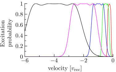
(a)
(b)

Figure 4: (Color online) (a) The excitation probability of atoms in state $|1\rangle$ against velocity $v$ by STIRAP pulses of different coupling parameters according to set (23). (b) The velocity spread $\Delta v$ decreases from the initial $3v_{\mathrm{rec}}$ to $0.1v_{\mathrm{rec}}$ of cooled ensemble.

The first step of a cooling cycle consists in transferring atoms from state $|1\rangle$ to $|3\rangle$ due to STIRAP pulse. Once the adiabaticity criterion (9) is fulfilled, atoms at the resonant velocity $v_{0}$ (4) are transferred with efficiency near unity. For laser configuration depicted in Fig. 1, atoms after the transfer get a momentum gain of $2\hbar k$ along $Oz$, so one should follow with a condition $v_{0}<0$. Because the spread of the resonant-velocity group is defined by Eq. (18), atoms at zero velocity are suppressed from the transfer when

$$v_{0}\leq-\dfrac{\Omega_{P0}^{2}}{4k|\Delta_{P}|}\quad\mbox{if $\Delta_{P}>0$},\quad v_{0}\leq-\dfrac{\Omega_{S0}^{2}}{4k|\Delta_{P}|}\quad\mbox{if $\Delta_{P}<0$}.$$ (21)

The inequality (21) only imposes a constraint on maximal magnitude of Rabi frequencies and thereby of the velocity spread of the resonant atoms. By decreasing Rabi frequency $\Omega_{S0}$ or $\Omega_{P0}$, the magnitude of the resonant velocity can be chosen substantially smaller than the recoil velocity. As a result, STIRAP can be efficiently used as the first step of an elementary cooling cycle. But such a transfer does not need the exact holding of the pulse duration, as that does in the standard Raman cooling Kasevich1992 .

In the second step, optical pumping excites atoms from $|3\rangle$ to $|2\rangle$ state, changing the momentum of an atom from $p^{\prime}$ to $p^{\prime}-\hbar k$. Then the atom spontaneously decays in the initial state $|1\rangle$, and its momentum becomes $p=p^{\prime}-\hbar k-\Delta p$ where $\Delta p$ is the projection of a spontaneously emitted photon; $|\Delta p|\leq\hbar k$. The resulting population in state $|1\rangle$ is written as

$$\langle 1,p|\sigma^{\prime}|1,p\rangle=\langle 1,p|\sigma|1,p\rangle+\langle 3,p{+}\hbar k{+}\Delta p|\sigma|3,p{+}\hbar k{+}\Delta p\rangle.$$

In turn, the density-matrix element $\sigma_{ij}(p)$ (19) corresponds to the momentum family $\mathcal{F}(p)$ that includes states $|a_{i}\rangle$ and $|a_{j}\rangle$, which leads to expression

$$\sigma^{\prime}_{11}(p)=\sigma_{11}(p)+\sigma_{33}(p-\hbar k+\Delta p),$$ (22)

where the momentum shift is given against $\mathcal{F}(p)$. Equation (22) demonstrates the mixing of different families $\mathcal{F}(p)$ due to spontaneous decay. After the cooling cycle the number of atoms at zero velocity increases together with the cooling of the atomic ensemble.

VII Comparison of two cooling types

(a)
(b)

Figure 5: (a) The excitation probability of atoms in state $|1\rangle$ against velocity $v$ by STIRAP pulse (24a) with the maximum at the resonant velocity $v_{0}=-0.25v_{\mathrm{rec}}$. (b) The velocity spread $\Delta v$ decreases from the initial $3v_{\mathrm{rec}}$ to $0.1v_{\mathrm{rec}}$ of cooled ensemble.

In this section, we compare two different variants of cooling by STIRAP. The first one uses the similar laser beams with $\Omega_{P0}=\Omega_{S0}$, so the velocity profile of the pulse has a symmetric shape. A condition when atoms at zero velocity are not transferred is derived from Eq. (21), and is written as

$$\Omega_{P0}^{2}=\Omega_{S0}^{2}=4k|v_{0}||\Delta_{P}|.$$

Both the pump and the Stokes pulse has the same pulse shape, so

$$T_{P}=T_{S}=0.5(t_{P}-t_{S}).$$

As the resonant velocity $v_{0}$ gets closer to zero, the width of the excitation profile decreases. To entirely excite the wing of the initial profile of spread $3v_{\text{rec}}$, we use a set of $v_{0}$

$$|v_{0}|=4v_{\text{rec}}/2^{k},\quad k=0,\dots,4,$$ (23)

for which the probability of transfer from state $|1\rangle$ is shown in Fig. 4(a). Note that as $|v_{0}|$ decreases, the magnitudes $\Omega_{P0}^{2}/|\Delta_{P}|$ and $\Omega_{S0}^{2}/|\Delta_{P}|$ decrease as well, which in turn leads to an increase of $\Delta\tau$ in order to fulfil the adiabaticity criterion (9). After the set has been applied, laser beams are alternated in order to excite the right-side profile. Such a cooling method is similar to ordinary Raman cooling.

In the second variant, the complete wing of initial distribution except a narrow peak at zero velocity is transferred by one STIRAP pulse as shown in Fig. 5(a). The peak width is defined by the resonant velocity $v_{0}$ which is equal to $-0.25v_{\mathrm{rec}}$. Notice that such an excitation is not attainable for ordinary Raman cooling, and represents a new type of a velocity-selective transfer with an essentially asymmetric profile. The advantage is in utilizing a single profile instead of the set (23). Rabi frequencies are given by

$$\Omega_{P0}^{2}=4k|v_{0}||\Delta_{P}|,\Omega_{S0}=8\Omega_{P0}\quad\mbox{if $\Delta_{P}>0$},$$ (24a)

$$\Omega_{S0}^{2}=4k|v_{0}||\Delta_{P}|,\Omega_{P0}=8\Omega_{S0}\quad\mbox{if $\Delta_{P}<0$}.$$ (24b)

Because a pulse of the largest amplitude should decrease faster, pulse widths are given by

$$T_{P}=0.5(t_{P}-t_{S}),T_{S}=0.35(t_{P}-t_{S})\quad\mbox{if $\Delta_{P}>0$},$$

$$T_{P}=0.35(t_{P}-t_{S}),T_{S}=0.5(t_{P}-t_{S})\quad\mbox{if $\Delta_{P}<0$}.$$

After each STIRAP pulse, laser beams are alternated giving the same excitation of the right side of the velocity distribution.

In both cooling variants, the duration $T_{\mathrm{pulse}}$ of STIRAP pulse is defined by the start and end time

$$t_{\mathrm{start}}=t_{S}-(t_{P}-t_{S}),\quad t_{\mathrm{end}}=t_{P}+(t_{P}-t_{S}),$$

being equal to $3(t_{P}-t_{S})$. Pulse durations in the first variant in accordance with the set (23) are given by

$$T_{\mathrm{pulse}}=6\cdot 2^{k}\tau_{R}\quad k=0,\dots,4,$$

where $\tau_{R}=\omega_{R}^{-1}$ is the recoil time. In the second variant, each pulse has the same duration equal to $96\tau_{R}$.

Figures 4(b) and 5(b) show results of both cooling methods starting from the initial distribution with the spread of $3v_{\mathrm{rec}}$. The velocity spread $\Delta v=(\mathrm{FWHM})/\sqrt{8\ln 2}$ has been reduced to nearly a) $0.06v_{\mathrm{rec}}$ in Fig. 4(b), and b) $0.04v_{\mathrm{rec}}$ in Fig. 5(b). The corresponding temperatures of the atomic ensemble have gone down to a) $0.004T_{\mathrm{rec}}$, and a) $0.002T_{\mathrm{rec}}$, where $T_{\mathrm{rec}}$ is the recoil-limit temperature. The duration of optical pumping is considered as a negligible value against that of STIRAP pulse, which in turn gives total durations of cooling methods as $7440\tau_{R}$ and $7680\tau_{R}$, respectively. In spite of the fact that both durations are approximately equal, the number of cooling cycles are rather different: the first method contains $N=200$ elementary cycles, whereas the second one contains $N=80$ cycles. For instance, being applied for cesium atoms ($\omega_{R}\sim 2\pi\times 2\mbox{kHz}$), both cooling variants take a time of $0.6\mathrm{s}$.

VIII Conclusion

We have described Raman cooling by velocity-selective STIRAP in the case of large upper-level detuning. We assume that the adiabaticity criterion is fulfilled for atoms in the two-photon resonance, so these atoms are transferred with efficiency that approaches unity. The position and width of the excitation profile is insensitive to the pulse duration, being in a linear dependence on the two-photon Rabi frequencies. This profile can take an asymmetric form, exciting the wing of the velocity distribution with the exception of a narrow peak near zero-velocity group. We have compared such a type of STIRAP with that of symmetric profile where a set of different coupling parameter utilized for excitation of the wing of the velocity distribution. Both methods has well-controlled the excitation probability, making the attainable temperatures essentially go below the one-photon recoil limit.

Our simplified treatment does not necessarily take into account many aspects of an actual experiment, but it shows that a priori the idea of Raman cooling combined with STIRAP offers a tool for reaching ultracold temperatures without the use of evaporative cooling. This is an example of robust quantum control of translational atomic degrees of freedom. If subjected to trapped atoms, 1D cooling eventually leads to cooling at higher dimensions, although at tight confinement the quantization of motion opens the door for sideband cooling (which also relies on a Raman process) Ye2008 ; Kerman1999 . It can also be applied to low-dimensional systems prepared with optical lattices Bloch2005 , such as the elongated quasi-1D cigar-shaped clouds in which the lattice provides tight confinement in perpendicular direction but atoms are almost free to move in axial direction, in which one can then apply Raman cooling. If using such a system as a wave guide, the trapping potential in axial direction is quite weak, which limits the use of side-band cooling in axial direction. Also, for atomic clocks one needs high numbers of atoms and yet low densities to avoid interaction-induced frequency shifts, and one solution is again an optical lattice that slices the sample into non-interacting 2D pancakes Derevianko2011 . Although then narrow-band cooling is the basic tool for e.g. alkaline earth atoms, one can also consider cooling at higher-lying atomic energy levels, which gives a rich level structure and opens the possibility for Raman cooling with tripod configuration. Finally, we note that the very recent interest in sub-Doppler cooling of fermionic isotopes Gokhroo2011 ; Landini2011 provides yet another application for non-evaporative cooling methods.

IX Acknowledgments

This research was supported by the Finnish Academy of Science and Letters, CIMO, the Academy of Finland, grant 133682, by the Ministry of Education and Science of the Russian Federation, grant RNP 2.1.1/2166, and by the Russian Foundation for Basic Research, grant RFBR 09-02-00223-a.

References

- (1) H. Mabuchi and A. C. Doherty, Science 298, 1372 (2002).
- (2) I. Bloch, Nature 453, 1016 (2008).
- (3) I. Bloch, J. Dalibard, and W. Zwerger, Rev. Mod. Phys. 80, 885 (2008).
- (4) H. Metcalf and P. van der Straten, Laser Cooling and Trapping, Springer-Verlag, Berlin, 1999.
- (5) M. Weidemüller and C. Zimmermann (eds.), Cold Atoms and Molecules, Wiley-VCH, Weinheim, 2009.
- (6) C. Cohen-Tannoudji and D. Guéry-Odelin, Advances in Atomic Physics: An Overview, World Scientific, Singapore, 2011.
- (7) C. J. Pethick and H. Smith, Bose-Einstein Condensation in Dilute Gases, 2nd Ed. (Cambridge University Press, Cambridge, 2008).
- (8) M.J. Holland, K.-A. Suominen, and K. Burnett, Phys. Rev. A 50, 1513 (1994).
- (9) K.-A. Suominen, J. Phys. B 29, 5981 (1996).
- (10) A. M. Steane, M. Chowdhury, and C. J. Foot, J. Opt. Soc. Am. B 9, 2142 (1992).
- (11) C. J. Cooper, G. Hillebrand, J. Rink, C. G. Townsend, K. Zetie, and C. J. Foot, Europhys. Lett 28, 397 (1994).
- (12) P. M. Duarte, R. A. Hart, J. M. Hitchcock, T. A. Corcovilos, T.-L. Yang, A. Reed, and R. G. Hulet, Phys. Rev. A 84, 061406(R) (2011).
- (13) D. C. McKay, D. Jervis, D. J. Fine, J. W. Simpson-Porco, G. J. A. Edge, and J. H. Thywissen, Phys. Rev. A 84, 063420 (2011).
- (14) J. Ye, H. J. Kimble, and H. Katori, Science 320, 1734 (2008).
- (15) A. Derevianko and H. Katori, Rev. Mod. Phys. 83, 331 (2011).
- (16) P. Phoonthong, P. Douglas, A. Wickenbrock, and F. Renzoni, Phys. Rev. A 82, 013406 (2010).
- (17) H. Theuer, R. G. Unanyan, C. Habscheid, K. Klein, and K. Bergmann, Opt. Express 4, 77 (1999).
- (18) F. Vewinger, M. Heinz, R. G. Fernandez, N. V. Vitanov, and K. Bergmann, Phys. Rev. Lett. 91, 213001 (2003).
- (19) N. V. Vitanov, T. Halfmann, B. W. Shore, and K. Bergmann, Annu. Rev. Phys. Chem. 52, 763 (2001).
- (20) B. M. Garraway and K.-A. Suominen, Phys. Rev. Lett. 80, 932 (1998).
- (21) M. Rodriguez, K.-A. Suominen, and B. M. Garraway, Phys. Rev. A 62, 053413 (2000).
- (22) M. Kasevich and S. Chu, Phys. Rev. Lett. 69, 1741 (1992).
- (23) N. Davidson, H. J. Lee, M. Kasevich, and S. Chu, Phys. Rev. Lett. 72, 3158 (1994).
- (24) J. Reichel, O. Morice, G. M. Tino, and C. Salomon, Europhys. Lett. 28, 477 (1994).
- (25) J. Reichel, F. Bardou, M. Ben Dahan, E. Peik, S. Rand, C. Salomon, and C. Cohen-Tannoudji, Phys. Rev. Lett. 75, 4575 (1995).
- (26) V. Boyer, L. J. Lising, S. L. Rolston, and W. D. Phillips, Phys. Rev. A 70, 043405 (2004).
- (27) V. S. Ivanov, Yu. V. Rozhdestvensky, and K.-A. Suominen, Phys. Rev. A 83, 023407 (2011).
- (28) E. Korsunsky, Phys. Rev. A 54, R1773 (1996).
- (29) A. Aspect, E. Arimondo, R. Kaiser, N. Vansteenkiste, and C. Cohen-Tannoudji, Phys. Rev. Lett. 61, 826 (1988).
- (30) A. Kuhn, H. Perrin, W. Hänsel, and Ch. Salomon, OSA TOPS on Ultracold Atoms and BEC 7, 58 (1996); arXiv:1109.5237v2 [cond-mat.quant-gas].
- (31) Hélène Perrin, Refroidissement d’atomes de césium confinés dans un piège dipolaire très désaccordé, Thèse de Doctorat, Université Paris VI, juin 1998.
- (32) H. Perrin, A. Kuhn, I. Bouchoule, T. Pfau and C. Salomon, Europhys. Lett. 46, 141 (1999).
- (33) U. Gaubatz, P. Rudecki, S. Schiemann, and K. Bergmann, J. Chem. Phys. 92, 5363 (1990).
- (34) K. Bergmann, H. Theuer, and B. W. Shore, Rev. Mod. Phys. 70, 1003 (1998).
- (35) M. Fewell, B. W. Shore, and K. Bergmann, Aust. J. Phys. 50, 281 (1997).
- (36) A. Messiah, Quantum Mechanics, North-Holland Publication, Amsterdam, 1962.
- (37) A. J. Kerman, V. Vuletić, C. Chin, and S. Chu, Phys. Rev. Lett. 84, 439 (2000).
- (38) I. Bloch, Nature Physics 1, 23 (2005).
- (39) V. Gokhroo, G. Rajalakshmi, R. K. Easwaran, and C. S. Unnikrishnan, J. Phys. B 44, 115307 (2011).
- (40) M. Landini, S. Roy, L. Carcagní, D. Trypogeorgos, M. Fattori, M. Inguscio, and G. Modugno, Phys. Rev. A 84, 043432 (2011).