Consensus of Multi-Agent Systems with General Linear and Lipschitz Nonlinear Dynamics Using Distributed Adaptive Protocols

Abstract

This paper considers the distributed consensus problems for multi-agent systems with general linear and Lipschitz nonlinear dynamics. Distributed relative-state consensus protocols with an adaptive law for adjusting the coupling weights between neighboring agents are designed for both the linear and nonlinear cases, under which consensus is reached for all undirected connected communication graphs. Extensions to the case with a leader-follower communication graph are further studied. In contrast to the existing results in the literature, the adaptive consensus protocols here can be implemented by each agent in a fully distributed fashion without using any global information.

I Introduction

In recent years, the consensus problem for multi-agent systems has received compelling attention from various scientific communities, for its potential applications in such broad areas as spacecraft formation flying, sensor networks, and cooperative surveillance [1, 2]. A general framework of the consensus problem for networks of integrator agents with fixed and switching topologies is addressed in [3]. The conditions given by [3] are further relaxed in [4]. A distributed algorithm is proposed in [5] to achieve consensus in finite time. Distributed $H_{\infty}$ consensus and control problems are investigated in [6, 7] for networks of agents subject to external disturbances and model uncertainties. Consensus algorithms are designed in [8, 9] for a group of agents with quantized communication links and limited data rate. The authors in [10] studies the controllability of leader-follower multi-agent systems from a graph-theoretic perspective. To ensure that the states of a group of agents follow a reference trajectory of a leader, consensus tracking algorithms are given in [11, 12] for agents with fixed and switching topologies. A passivity-based design framework is proposed in [13] to achieve group coordination. The consensus problems for networks of double- and high-order integrators are studied in [14, 15, 16]. Readers are referred to the recent surveys [1, 2] for a relatively complete coverage of the literature on consensus.

This paper considers the distributed consensus problems for multi-agent systems with general linear and Lipschitz nonlinear dynamics. Consensus of multi-agent systems with general linear dynamics was previously studied in [17, 18, 19, 20]. In particular, different static and dynamic consensus protocols are designed in [17, 18], requiring the smallest nonzero eigenvalue of the Laplacian matrix associated with the communication graph to be known by each agent to determine the bound for the coupling weight. However, the Laplacian matrix depends on the entire communication graph and is hence global information. In other words, these consensus protocols in [17, 18] can not be computed and implemented by each agent in a fully distributed fashion, i.e., using only local information of its own and neighbors. To tackle this problem, we propose here a distributed consensus protocol based on the relative states combined with an adaptive law for adjusting the coupling weights between neighboring agents, which is partly inspired by the edge-based adaptive strategy for the synchronization of complex networks in [21, 22].

The proposed distributed adaptive protocols are designed, respectively, for linear and Lipschitz nonlinear multi-agent systems, under which consensus is reached in both the linear and the nonlinear cases for any undirected connected communication graph. It is shown that a sufficient condition for the existence of such a protocol in the linear case is that each agent is stabilizable. Existence conditions for the adaptive protocol in the nonlinear case are also discussed. It is pointed out that the results in the nonlinear case can be reduced to those in the linear case, when the Lipschitz nonlinearity does not exist. Extensions of the obtained results to the case with a leader-follower communication graph are further discussed. It is worth noting that the consensus protocols in [19, 20] can also achieve consensus for all connected communication graphs. Contrary to the general linear and Lipschitz nonlinear agent dynamics in this paper, the linear agent dynamics in [19] are restricted to be neutrally stable and all the eigenvalues of the state matrix of each agent in [20] are assumed to lie in the closed left-half plane. In addition, adaptive synchronization of a class of complex network satisfying a Lipschitz-type condition is considered in [21, 22]. However, the results given in [21, 22] require the inner coupling matrix to be positive semi-definite, which is not directly applicable to the consensus problem under investigation here.

The rest of this paper is organized as follows. The adaptive consensus problems for multi-agent systems with general linear and Lipschitz nonlinear dynamics are considered, respectively, in Sections II and III. Extensions to the case with a leader-follower communication graph are studied in Section IV. Simulation examples are presented to illustrate the analytical results in Section V. Conclusions are drawn in Section VI.

Throughout this paper, the following notations will be used: Let $\mathbf{R}^{n\times n}$ be the set of $n\times n$ real matrices. The superscript $T$ means transpose for real matrices. $I_{N}$ represents the identity matrix of dimension $N$. Matrices, if not explicitly stated, are assumed to have compatible dimensions. Denote by $\mathbf{1}$ the column vector with all entries equal to one. $\mathrm{diag}(A_{1},\cdots,A_{n})$ represents a block-diagonal matrix with matrices $A_{i},i=1,\cdots,n,$ on its diagonal. For real symmetric matrices $X$ and $Y$, $X>(\geq)Y$ means that $X-Y$ is positive (semi-)definite. $A\otimes B$ denotes the Kronecker product of matrices $A$ and $B$.

II Adaptive Consensus for Multi-Agent Systems with General Linear Dynamics

Consider a group of $N$ identical agents with general linear dynamics. The dynamics of the $i$-th agent are described by

$$\dot{x}_{i} =Ax_{i}+Bu_{i},\quad i=1,\cdots,N,$$ (1)

where $x_{i}\in\mathbf{R}^{n}$ is the state, $u_{i}\in\mathbf{R}^{p}$ is the control input, and $A$, $B$, are constant matrices with compatible dimensions.

The communication topology among the agents is represented by an undirected graph $\mathcal{G}=(\mathcal{V},\mathcal{E})$, where $\mathcal{V}=\{1,\cdots,N\}$ is the set of nodes (i.e., agents), and $\mathcal{E}\subset\mathcal{V}\times\mathcal{V}$ is the set of edges. An edge $(i,j)$ $(i\neq j)$ means that agents $i$ and $j$ can obtain information from each other. A path in $\mathcal{G}$ from node $i_{1}$ to node $i_{l}$ is a sequence of edges of the form $(i_{k},i_{k+1})$, $k=1,\cdots,l-1$. An undirected graph is connected if there exists a path between every pair of distinct nodes, otherwise is disconnected.

A variety of static and dynamic consensus protocols have been proposed to reach consensus for agents with dynamics given by (1), e.g., in [17, 18, 19, 20]. For instance, a static consensus protocol based on the relative states between neighboring agents is given in [17] as

$$u_{i}=cK\sum_{j=1}^{N}a_{ij}(x_{i}-x_{j}),\quad i=1,\cdots,N,$$ (2)

where $c>0$ is the coupling weight among neighboring agents, $K\in\mathbf{R}^{p\times n}$ is the feedback gain matrix, and $a_{ij}$ is $(i,j)$-th entry of the adjacency matrix $\mathcal{A}$ associated with $\mathcal{G}$, defined as $a_{ii}=0$, $a_{ij}=a_{ji}=1$ if $(j,i)\in\mathcal{E}$ and $a_{ij}=a_{ji}=0$ otherwise. The Laplacian matrix $\mathcal{L}=(\mathcal{L}_{ij})_{N\times N}$ of $\mathcal{G}$ is defined by $\mathcal{L}_{ii}=\sum_{j=1,j\neq i}^{N}a_{ij}$ and $\mathcal{L}_{ij}=-a_{ij}$ for $i\neq j$.

Lemma 1 ([17])

Suppose that $\mathcal{G}$ is connected. The $N$ agents described by (1) reach consensus (i.e., $\lim_{t\rightarrow\infty}\|x_{i}(t)-x_{j}(t)\|=0$, $\forall\,i,j=1,\cdots,N$) under the protocol (2) with $K=-B^{T}P^{-1}$ and the coupling weight $c\geq\frac{1}{\lambda_{2}}$, where $\lambda_{2}$ is the smallest nonzero eigenvalue of $\mathcal{L}$ and $P>0$ is a solution to the following linear matrix inequality (LMI):

$$AP+PA^{T}-2BB^{T}<0.$$ (3)

As shown in the above lemma, the coupling weight $c$ should be not less than the inverse of the smallest nonzero eigenvalue $\lambda_{2}$ of $\mathcal{L}$ to reach consensus. The design method for the dynamic protocol in [18] depends on $\lambda_{2}$ also. However, $\lambda_{2}$ is global information in the sense that each agent has to know the Laplacian matrix and hence the entire communication graph $\mathcal{G}$ to compute it. Therefore, the consensus protocols given in Lemma 1 and [18] cannot be implemented by each agent in a fully distributed fashion, i.e., using only the local information of its own and neighbors.

In order to avoid the limitation stated as above, we propose the following distributed consensus protocol with an adaptive law for adjusting the coupling weights:

$$u_{i} =F\sum_{j=1}^{N}c_{ij}a_{ij}(x_{i}-x_{j}),$$ (4)

$$\dot{c}_{ij} =\kappa_{ij}a_{ij}(x_{i}-x_{j})^{T}\Gamma(x_{i}-x_{j}),\quad i=1,\cdots,N,$$

where $a_{ij}$ is defined as in (2), $\kappa_{ij}=\kappa_{ji}$ are positive constants, $c_{ij}$ denotes the time-varying coupling weight between agents $i$ and $j$ with $c_{ij}(0)=c_{ji}(0)$, and $F\in\mathbf{R}^{p\times n}$ and $\Gamma\in\mathbf{R}^{n\times n}$ are feedback gain matrices.

We next design $F$ and $\Gamma$ in (4) such that the $N$ agents reach consensus.

Theorem 1

For any given connected graph $\mathcal{G}$, the $N$ agents described by (1) reach consensus under the protocol (4) with $F=-B^{T}P^{-1}$ and $\Gamma=P^{-1}BB^{T}P^{-1}$, where $P>0$ is a solution to the LMI (3). Moreover, each coupling weight $c_{ij}$ converges to some finite steady-state value.

Proof:

Let $\bar{x}=\frac{1}{N}\sum_{j=1}^{N}x_{j}$, $e_{i}=x_{i}-\bar{x}$, and $e=[e_{1}^{T},\cdots,e_{N}^{T}]^{T}$. Then, we get $e=\left((I_{N}-\frac{1}{N}\mathbf{1}\mathbf{1}^{T})\otimes I_{n}\right)x.$ It is easy to see that $0$ is a simple eigenvalue of $I_{N}-\frac{1}{N}\mathbf{1}\mathbf{1}^{T}$ with $\mathbf{1}$ as the corresponding right eigenvector, and 1 is the other eigenvalue with multiplicity $N-1$. Then, it follows that $e=0$ if and only if $x_{1}=\cdots=x_{N}$. Therefore, the consensus problem under the protocol (4) can be reduced to the asymptotical stability of $e$. Using (4) for (1), it follows that $e$ satisfies the following dynamics:

$$\dot{e}_{i} =Ae_{i}+\sum_{j=1}^{N}c_{ij}a_{ij}BF(e_{i}-e_{j}),$$ (5)

$$\dot{c}_{ij} =\kappa_{ij}a_{ij}(e_{i}-e_{j})^{T}\Gamma(e_{i}-e_{j}),\quad i=1,\cdots,N.$$

Consider the Lyapunov function candidate

$$V_{1}=\sum_{i=1}^{N}e_{i}^{T}P^{-1}e_{i}+\sum_{i=1}^{N}\sum_{j=1,j\neq i}^{N}\frac{(c_{ij}-\alpha)^{2}}{2\kappa_{ij}},$$ (6)

where $\alpha$ is a positive constant. The time derivative of $V_{1}$ along the trajectory of (5) is given by

$$\dot{V}_{1} =2\sum_{i=1}^{N}e_{i}^{T}P^{-1}\dot{e}_{i}+\sum_{i=1}^{N}\sum_{j=1,j\neq i}^{N}\frac{c_{ij}-\alpha}{\kappa_{ij}}\dot{c}_{ij}$$ (7)

$$=2\sum_{i=1}^{N}e_{i}^{T}P^{-1}\left(Ae_{i}+\sum_{j=1}^{N}c_{ij}a_{ij}BF(e_{i}-e_{j})\right)$$

$$\quad+\sum_{i=1}^{N}\sum_{j=1,j\neq i}^{N}(c_{ij}-\alpha)a_{ij}(e_{i}-e_{j})^{T}\Gamma(e_{i}-e_{j}).$$

Because $\kappa_{ij}=\kappa_{ji}$, $c_{ij}(0)=c_{ji}(0)$, and $\Gamma$ is symmetric, it follows from (4) that $c_{ij}(t)=c_{ji}(t)$, $\forall\,t\geq 0$. Therefore, we have

$$\sum_{i=1}^{N}\sum_{j=1,j\neq i}^{N}(c_{ij}-\alpha)a_{ij}(e_{i}-e_{j})^{T}\Gamma(e_{i}-e_{j})$$ (8)

$$\quad\qquad=2\sum_{i=1}^{N}\sum_{j=1}^{N}(c_{ij}-\alpha)a_{ij}e_{i}^{T}\Gamma(e_{i}-e_{j}).$$

Let $\tilde{e}_{i}=P^{-1}e_{i}$ and $\tilde{e}=[\tilde{e}_{1}^{T},\cdots,\tilde{e}_{N}^{T}]^{T}$. Substituting $F=-B^{T}P^{-1}$ and $\Gamma=P^{-1}BB^{T}P^{-1}$ into (7), we can obtain

$$\dot{V}_{1} =2\sum_{i=1}^{N}e_{i}^{T}P^{-1}Ae_{i}-2\alpha\sum_{i=1}^{N}\sum_{j=1}^{N}a_{ij}e_{i}^{T}P^{-1}BB^{T}P^{-1}(e_{i}-e_{j})$$ (9)

$$=\sum_{i=1}^{N}\tilde{e}_{i}^{T}(AP+PA^{T})\tilde{e}_{i}-2\alpha\sum_{i=1}^{N}\sum_{j=1}^{N}\mathcal{L}_{ij}\tilde{e}_{i}^{T}BB^{T}\tilde{e}_{j}$$

$$=\tilde{e}^{T}\left(I_{N}\otimes(AP+PA^{T})-2\alpha\mathcal{L}\otimes BB^{T}\right)\tilde{e},$$

where $\mathcal{L}$ is the Laplacian matrix associated with $\mathcal{G}$.

Because $\mathcal{G}$ is connected, zero is a simple eigenvalue of $\mathcal{L}$ and all the other eigenvalues are positive [23]. Let $U\in\mathbf{R}^{N\times N}$ be such a unitary matrix that $U^{T}\mathcal{L}U=\Lambda\triangleq{\mathrm{diag}}(0,\lambda_{2},\cdots,\lambda_{N})$. Because the right and left eigenvectors of $\mathcal{L}$ corresponding to the zero eigenvalue are ${\bf 1}$ and ${\bf 1}^{T}$, respectively, we can choose $U=\left[\begin{smallmatrix}\frac{\mathbf{1}}{\sqrt{N}}&Y_{1}\end{smallmatrix}\right]$ and $U^{T}=\left[\begin{smallmatrix}\frac{\mathbf{1}^{T}}{\sqrt{N}}\\ Y_{2}\end{smallmatrix}\right]$, with $Y_{1}\in\mathbf{R}^{N\times(N-1)}$ and $Y_{2}\in\mathbf{R}^{(N-1)\times N}$. Let $\xi\triangleq[\xi_{1}^{T},\cdots,\xi_{N}^{T}]^{T}=(U^{T}\otimes I_{n})\tilde{e}$. By the definitions of $e$ and $\tilde{e}$, it is easy to see that

$$\xi_{1}=(\frac{\mathbf{1}^{T}}{\sqrt{N}}\otimes I_{n})\tilde{e}=(\frac{\mathbf{1}^{T}}{\sqrt{N}}\otimes P^{-1})e=0.$$ (10)

Then, we have

$$\dot{V}_{1} =\xi^{T}\left(I_{N}\otimes(AP+PA^{T})-2\alpha\Lambda\otimes BB^{T}\right)\xi$$ (11)

$$=\sum_{i=2}^{N}\xi_{i}^{T}\left(AP+PA^{T}-2\alpha\lambda_{i}BB^{T}\right)\xi_{i}.$$

By choosing $\alpha$ sufficiently large such that $\alpha\lambda_{i}\geq 1$, $i=2,\cdots,N$, it follows from (3) that

$$AP+PA^{T}-2\alpha\lambda_{i}BB^{T}\leq AP+PA^{T}-2BB^{T}<0.$$

Therefore, $\dot{V}_{1}\leq 0$.

Since $\dot{V}_{1}\leq 0$, $V_{1}(t)$ is bounded and so is each $c_{ij}$. By noting $\Gamma\geq 0$, it can be seen from (5) that $c_{ij}$ is monotonically increasing. Then, it follows that each coupling weight $c_{ij}$ converges to some finite value. Let $S=\{\xi_{i},c_{ij}|\dot{V}_{1}=0\}$. Note that $\dot{V}_{1}\equiv 0$ implies that $\xi_{i}=0$, $i=2,\cdots,N$, which, by noticing that $\xi_{1}\equiv 0$ in (10), further implies that $\tilde{e}=0$ and $e=0$. Hence, by LaSalle’s Invariance principle [24], it follows that $e(t)\rightarrow 0$, as $t\rightarrow\infty$. That is, the consensus problem is solved. ∎

Remark 1

Equation (4) presents an adaptive protocol, under which the agents with dynamics given by (1) can reach consensus for all connected communication topologies. In contrast to the consensus protocols in [17, 18], the adaptive protocol (4) can be computed and implemented by each agent in a fully distributed way. As shown in [17], a necessary and sufficient condition for the existence of a $P>0$ to the LMI (3) is that $(A,B)$ is stabilizable. Therefore, a sufficient condition for the existence of a protocol (4) satisfying Theorem 1 is that $(A,B)$ is stabilizable.

Remark 2

It is worth noting that the consensus protocols in [19, 20] can also achieve consensus for all connected communication graphs. Contrary to the general linear agent dynamics in this section, the agent dynamics in [19] are restricted to be neutrally stable and all the eigenvalues of the state matrix of each agent in [20] are assumed to lie in the closed left-half plane.

III Adaptive Consensus for Multi-Agent Systems with Lipschitz Nonlinearity

In this section, we study the consensus problem for a group of $N$ identical nonlinear agents, described by

$$\dot{x}_{i}=Ax_{i}+D_{1}f(x_{i})+Bu_{i},\qquad i=1,\cdots,N,$$ (12)

where $x_{i}\in\mathbf{R}^{n}$, $u_{i}\in\mathbf{R}^{p}$ are the state and the control input of the $i$-th agent, respectively, $A$, $B$, $D_{1}$, are constant matrices with compatible dimensions, and the nonlinear function $f(x_{i})$ is assumed to satisfy the Lipschitz condition with a Lipschitz constant $\gamma>0$, i.e.,

$$\|f(x)-f(y)\|\leq\gamma\|x-y\|,\quad\forall\,x,y\in\mathbf{R}^{n}.$$ (13)

Theorem 2

Solve the following LMI:

$$\begin{bmatrix}AQ+QA^{T}-\tau BB^{T}+\gamma^{2}D_{1}TD_{1}^{T}&Q\\ Q&-T\end{bmatrix}<0,$$ (14)

to get a matrix $Q>0$, a scalar $\tau>0$ and a diagonal matrix $T>0$. Then, the $N$ agents described by (12) reach global consensus under the protocol (4) with $F=-B^{T}Q^{-1}$ and $\Gamma=Q^{-1}BB^{T}Q^{-1}$ for any connected communication graph $\mathcal{G}$. Furthermore, each coupling weight $c_{ij}$ converges to some finite steady-state value.

Proof:

Using (4) for (12), we obtain the closed-loop network dynamics as

$$\dot{x}_{i} =Ax_{i}+D_{1}f(x_{i})+\sum_{j=1}^{N}c_{ij}a_{ij}BF(x_{i}-x_{j}),$$ (15)

$$\dot{c}_{ij} =\kappa_{ij}a_{ij}(x_{i}-x_{j})^{T}\Gamma(x_{i}-x_{j}),\quad i=1,\cdots,N.$$

As argued in the Proof of Theorem 1, it follows that $c_{ij}(t)=c_{ji}(t)$, $\forall\,t\geq 0$.

Letting $\bar{x}=\frac{1}{N}\sum_{j=1}^{N}x_{j}$, $e_{i}=x_{i}-\bar{x}$, and $e=[e_{1}^{T},\cdots,e_{N}^{T}]^{T}$, we get $e=\left((I_{N}-\frac{1}{N}\mathbf{1}\mathbf{1}^{T})\otimes I_{n}\right)x.$ By following similar steps to those in Theorem 1, we can reduce the consensus problem of (15) to the convergence of $e$ to the origin. It is easy to obtain that $e$ satisfies the following dynamics:

$$\dot{e}_{i} =Ae_{i}+D_{1}f(x_{i})-\frac{1}{N}\sum_{j=1}^{N}D_{1}f(x_{j})+\sum_{j=1}^{N}(\tilde{c}_{ij}+\beta)a_{ij}BF(e_{i}-e_{j}),$$ (16)

$$\dot{\tilde{c}}_{ij} =\kappa_{ij}a_{ij}(e_{i}-e_{j})^{T}\Gamma(e_{i}-e_{j}),\quad i=1,\cdots,N,$$

where $c_{ij}=\tilde{c}_{ij}+\beta$ and $\beta$ is a positive constant.

Consider the Lyapunov function candidate

$$V_{2}=\sum_{i=1}^{N}e_{i}^{T}Q^{-1}e_{i}+\sum_{i=1}^{N}\sum_{j=1,j\neq i}^{N}\frac{\tilde{c}_{ij}^{2}}{2\kappa_{ij}}.$$ (17)

The time derivative of $V_{2}$ along the trajectory of (16) is

$$\dot{V}_{2} =2\sum_{i=1}^{N}e_{i}^{T}Q^{-1}\dot{e}_{i}+\sum_{i=1}^{N}\sum_{j=1,j\neq i}^{N}\frac{\tilde{c}_{ij}}{\kappa_{ij}}\dot{\tilde{c}}_{ij}$$ (18)

$$=2\sum_{i=1}^{N}e_{i}^{T}Q^{-1}\left(Ae_{i}+D_{1}f(x_{i})-\frac{1}{N}\sum_{j=1}^{N}D_{1}f(x_{j})+\sum_{j=1}^{N}(\tilde{c}_{ij}+\beta)a_{ij}BF(e_{i}-e_{j})\right)$$

$$\quad+\sum_{i=1}^{N}\sum_{j=1,j\neq i}^{N}\tilde{c}_{ij}a_{ij}(e_{i}-e_{j})^{T}\Gamma(e_{i}-e_{j})$$

$$=2\sum_{i=1}^{N}e_{i}^{T}Q^{-1}Ae_{i}-2\beta\sum_{i=1}^{N}\sum_{j=1}^{N}\mathcal{L}_{ij}e_{i}^{T}Q^{-1}BB^{T}Q^{-1}e_{j}$$

$$\quad+2\sum_{i=1}^{N}e_{i}^{T}Q^{-1}D_{1}\left(f(x_{i})-f(\bar{x})+f(\bar{x})-\frac{1}{N}\sum_{j=1}^{N}f(x_{j})\right),$$

where we have used the fact (8) to get the last equation.

Using the Lipschitz condition (13) gives

$$2e_{i}^{T}Q^{-1}D_{1}(f(x_{i})-f(\bar{x})) \leq 2\gamma\|e_{i}^{T}Q^{-1}D_{1}T^{\frac{1}{2}}\|\|T^{-\frac{1}{2}}e_{i}\|$$ (19)

$$\leq e_{i}^{T}(\gamma^{2}Q^{-1}D_{1}TD_{1}^{T}Q^{-1}+T^{-1})e_{i},$$

where $T$ is given in (14). Because $\sum_{i=1}^{N}e_{i}^{T}=0$, we have

$$\sum_{i=1}^{N}e_{i}^{T}Q^{-1}D_{1}\left(f(\bar{x})-\frac{1}{N}\sum_{j=1}^{N}f(x_{j})\right)=0.$$ (20)

Let $\hat{e}_{i}=Q^{-1}e_{i}$ and $\hat{e}=[\hat{e}_{1}^{T},\cdots,\hat{e}_{N}^{T}]^{T}$. In virtue of (19) and (20), we can obtain from (18) that

$$\dot{V}_{2} \leq\sum_{i=1}^{N}\hat{e}_{i}^{T}\left((AQ+QA^{T}+\gamma^{2}D_{1}TD_{1}^{T}+QT^{-1}Q)\hat{e}_{i}-2\beta\sum_{j=1}^{N}\mathcal{L}_{ij}BB^{T}\hat{e}_{j}\right)$$ (21)

$$=\hat{e}^{T}\left(I_{N}\otimes(AQ+QA^{T}+\gamma^{2}D_{1}TD_{1}^{T}+QT^{-1}Q)-2\beta\mathcal{L}\otimes BB^{T}\right)\hat{e}.$$

Let $U\in\mathbf{R}^{N\times N}$ be the unitary matrix defined in the proof of Theorem 1, satisfying $U^{T}\mathcal{L}U=\Lambda={\mathrm{diag}}(0,\lambda_{2},\cdots,\lambda_{N})$. Let $\zeta\triangleq[\zeta_{1}^{T},\cdots,\zeta_{N}^{T}]^{T}=(U^{T}\otimes I_{n})\hat{e}$. Clearly, $\zeta_{1}=(\frac{\mathbf{1}^{T}}{\sqrt{N}}\otimes Q^{-1})e=0$. From (21), we have

$$\dot{V}_{2} \leq\zeta^{T}\left(I_{N}\otimes(AQ+QA^{T}+\gamma^{2}D_{1}TD_{1}^{T}+QT^{-1}Q)-2\beta\Lambda\otimes BB^{T}\right)\zeta$$ (22)

$$=\sum_{i=2}^{N}\zeta_{i}^{T}\left(AQ+QA^{T}+\gamma^{2}D_{1}TD_{1}^{T}+QT^{-1}Q-2\beta\lambda_{i}BB\right)\zeta_{i}$$

$$\triangleq W(\zeta).$$

By choosing $\beta$ sufficiently large such that $2\beta\lambda_{i}\geq\tau$, $i=2,\cdots,N$, it follows that

$$AQ+QA^{T}-2\beta\lambda_{i}BB^{T}+\gamma^{2}D_{1}TD_{1}^{T}+QT^{-1}Q$$

$$\qquad\qquad\leq AQ+QA^{T}-\tau BB^{T}+\gamma^{2}D_{1}TD_{1}^{T}+QT^{-1}Q$$

$$\qquad\qquad<0,\quad i=2,\cdots,N,$$

where the last inequality follows from (14) by using the Schur complement lemma [25]. Therefore, $W(\zeta)\leq 0$.

Since $\dot{V}_{2}\leq 0$, $V_{2}(t)$ is bounded and so is each $\tilde{c}_{ij}$. By (16), $\tilde{c}_{ij}$ is monotonically increasing. Then, it follows that each $\tilde{c}_{ij}$ converges to some finite value. Thus the coupling weights $c_{ij}$ converge to finite steady-state values. Note that $V_{2}$ is positive definite and radically unbounded. By LaSalle-Yoshizawa theorem [24], it follows that $\lim_{t\rightarrow\infty}W(\zeta)=0$, implying that $\zeta_{i}\rightarrow 0$, $i=2,\cdots,N$, as $t\rightarrow\infty$, which, together with $\zeta_{1}\equiv 0$, further implies that $e(t)\rightarrow 0$, as $t\rightarrow\infty$. This completes the proof. ∎

Remark 3

By using Finsler’s Lemma [26], it is not difficult to see that there exist a $Q>0$, a $T>0$ and a $\tau>0$ such that (14) holds if and only if there exists a $K$ such that $(A+BK)Q+Q(A+BK)^{T}+\gamma^{2}D_{1}TD_{1}^{T}+QT^{-1}Q<0$, which with $T=I$ is dual to the observer design problem for a single Lipschitz system in [27, 28]. According to Theorem 2 in [28], the LMI (14) is feasible, and thus there exists an adaptive protocol (4) reaching consensus, if the distance to unobservability of $(A,B)$ is larger than $\gamma$. Besides, a diagonal scaling matrix $T>0$ is introduced here in (14) to reduce conservatism. If the nonlinear function $f(x_{i})=0$ in (12), then (12) becomes (1). By choosing $T$ sufficiently large and letting $D_{1}=0$ and $\tau=2$, then (14) becomes $AQ+QA^{T}-2BB^{T}<0$. Therefore, for the case without the Lipschitz nonlinearity, Theorem 2 is reduced to Theorem 1.

Remark 4

It should be mentioned that the adaptive law in (4) for adjusting the coupling weights is inspired by the edge-based adaptive strategy in [21, 22], where adaptive synchronization of a class of complex network satisfying a Lipschitz-type condition is considered. However, the results given in [21, 22] require the inner coupling matrix to be positive semi-definite, and are thereby not directly applicable to the consensus problem under investigation here.

IV Extensions

The communication topology is assumed to be undirected in the previous sections, where the final consensus value reached by the agents is generally not explicitly known, due to the nonlinearity in the closed-loop network dynamics. In many practical cases, it is desirable for the agents’ states to asymptotically approach a reference state. In this section, we consider the case where a network of $N+1$ agents maintains a leader-follower communication structure.

The agents’ dynamics remain the same as in (1). The agents indexed by $1,\cdots,N$, are referred to as followers, while the agent indexed by 0 is called the virtual leader whose control input $u_{0}=0$. The communication topology among the $N$ followers is represented by an undirected graph $\mathcal{G}$. It is assumed that the leader receives no information from any follower and the state of the leader is available to only a subset of the followers (without loss of generality, the first $q$ followers). In this case, the following distributed consensus protocol is proposed

$$u_{i} =\hat{F}\left(\sum_{j=1}^{N}c_{ij}a_{ij}(x_{i}-x_{j})+c_{i}d_{i}(x_{i}-x_{0})\right),$$ (23)

$$\dot{c}_{ij} =\kappa_{ij}a_{ij}(x_{i}-x_{j})^{T}\hat{\Gamma}(x_{i}-x_{j}),$$

$$\dot{c}_{i} =\kappa_{i}d_{i}(x_{i}-x_{0})^{T}\hat{\Gamma}(x_{i}-x_{0}),\quad i=1,\cdots,N,$$

where $a_{ij}$, $c_{ij}$, $\kappa_{ij}$ are defined as in (4), $c_{i}$ denotes the coupling weight between agent $i$ and the virtual leader, $\kappa_{i}$ are positive constants, $\hat{F}\in\mathbf{R}^{p\times n}$ and $\hat{\Gamma}\in\mathbf{R}^{n\times n}$ are feedback gain matrices, and $d_{i}$ are constant gains, satisfying $d_{i}>0$, $i=1,\cdots,q,$ and $d_{i}=0$, $i=q+1,\cdots,N$.

The objective here is to design $\hat{F}\in\mathbf{R}^{p\times n}$ and $\hat{\Gamma}\in\mathbf{R}^{n\times n}$ such that the states of the followers can asymptotically approach the state of the leader in the sense that $\lim_{t\rightarrow\infty}\|x_{i}(t)-x_{0}(t)\|=0$, $\forall\,i=1,\cdots,N.$

Theorem 3

Assume that $\mathcal{G}$ is connected and at least one follower can have access to the leader’s state. Then, the states of the $N$ followers asymptotically approach the state of the leader, under the protocol (23) with $\hat{F}=-B^{T}P^{-1}$ and $\hat{\Gamma}=P^{-1}BB^{T}P^{-1}$, where $P>0$ is a solution to (3), and the coupling weights $c_{ij}$ and $c_{i}$ converge to finite values.

Proof:

Let $\varepsilon_{i}=x_{i}-x_{0}$, $i=1,\cdots,N$. Then, the collective network dynamics resulting from (1) and (23) can be written as

$$\dot{\varepsilon}_{i} =A\varepsilon_{i}+B\hat{F}\left(\sum_{j=1}^{N}c_{ij}a_{ij}(\varepsilon_{i}-\varepsilon_{j})+c_{i}d_{i}\varepsilon_{i}\right),$$ (24)

$$\dot{c}_{ij} =\kappa_{ij}a_{ij}(\varepsilon_{i}-\varepsilon_{j})^{T}\hat{\Gamma}(\varepsilon_{i}-\varepsilon_{j}),$$

$$\dot{c}_{i} =\kappa_{i}d_{i}\varepsilon_{i}^{T}\hat{\Gamma}\varepsilon_{i},\quad i=1,\cdots,N.$$

Clearly, the states of the followers under (23) can asymptotically approach the state of the leader, if (24) is asymptotically stable.

Consider the Lyapunov function candidate

$$V_{3}=\sum_{i=1}^{N}\varepsilon_{i}^{T}P^{-1}\varepsilon_{i}+\sum_{i=1}^{N}\sum_{j=1,j\neq i}^{N}\frac{(c_{ij}-\beta)^{2}}{2\kappa_{ij}}+\sum_{i=1}^{N}\frac{(c_{i}-\beta)^{2}}{\kappa_{i}},$$ (25)

where $\beta$ is a positive constant. The rest of the proof follows similar steps to those in Theorem 1, and by further noting the fact: Suppose that $R=\mathrm{diag}(d_{1},d_{2},\cdots,d_{N})\geq 0$ with at least one diagonal item being positive. Then, $\mathcal{L}+R$ is positive definite if $\mathcal{G}$ is connected [11]. ∎

Remark 5

It is worth mentioning that an adaptive pinning scheme similar to (23) has been proposed in [29]. Compared to [29] where the inner coupling matrix is an identity matrix, the adaptive protocol (23) here is more general.

The case with the agents described by (12) can be discussed similarly, and is thus omitted here for brevity.

V Simulation Examples

In this section, a simulation example is provided to validate the effectiveness of the theoretical results.

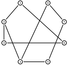
Figure 1: The communication topology.

Consider a network of single-link manipulators with revolute joints actuated by a DC motor. The dynamics of the $i$-th manipulator is described by (12), with (see [28])

$$x_{i} =\begin{bmatrix}x_{i1}\\ x_{i2}\\ x_{i3}\\ x_{i4}\end{bmatrix},\quad A=\begin{bmatrix}0&1&0&0\\ -48.6&-1.25&48.6&0\\ 0&0&0&10\\ 1.95&0&-1.95&0\end{bmatrix},\quad B=\begin{bmatrix}0\\ 21.6\\ 0\\ 0\end{bmatrix},$$

$$D_{1} =I_{4},\quad f(x_{i})=\begin{bmatrix}0&0&0&-0.333\mathrm{sin}(x_{i3})\end{bmatrix}^{T}.$$

Clearly, $f(x_{i})$ here satisfies (13) with a Lipschitz constant $\gamma=0.333$.

Solving the LMI (14) by using the LMI toolbox of Matlab gives the feedback gain matrices in (4) as

$$F =\begin{bmatrix}-1.8351&-0.2144&1.0309&-2.247\end{bmatrix},$$

$$\Gamma =\left[\begin{matrix}3.3676&0.3935&-1.8917&4.1236\\ 0.3935&0.046&-0.221&0.4818\\ -1.8917&-0.221&1.0627&-2.3164\\ 4.1236&0.4818&-2.3164&5.0492\end{matrix}\right].$$

To illustrate Theorem 2, let the communication graph $\mathcal{G}$ be given in Fig. 1. Here $\mathcal{G}$ is undirected and connected. Let $\kappa_{ij}=1$, $i,j=1,\cdots,8$, in (4), and $c_{ij}(0)=c_{ji}(0)$ be randomly chosen. The states trajectories of the eight manipulators under the protocol (4) are depicted in Fig. 2, from which it can be observed that consensus is reached. The coupling weights $c_{ij}$ are shown in Fig. 3, which converge to finite steady-state values.

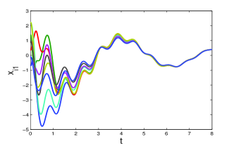
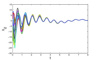
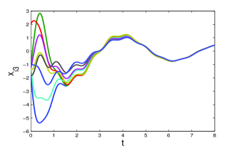
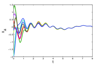
Figure 2: The states of the eight manipulators under (4).

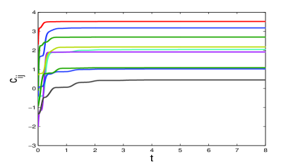
Figure 3: The coupling weights $c_{ij}$.

VI Conclusion

In this paper, the distributed consensus problems have been considered for multi-agent systems with general linear and Lipschitz nonlinear dynamics. Distributed relative-state consensus protocols with an adaptive law for adjusting the coupling weights between neighboring agents are designed for both the linear and nonlinear cases, under which consensus is reached for all undirected connected communication graphs. Extensions to the case with a leader-follower communication graph have also been studied.

References

• [1] R. Olfati-Saber, J. Fax, and R. Murray, “Consensus and cooperation in networked multi-agent systems,” Proceedings of the IEEE, vol. 95, no. 1, pp. 215–233, 2007.
• [2] W. Ren, R. Beard, and E. Atkins, “Information consensus in multivehicle cooperative control,” IEEE Control Systems Magazine, vol. 27, no. 2, pp. 71–82, 2007.
• [3] R. Olfati-Saber and R. Murray, “Consensus problems in networks of agents with switching topology and time-delays,” IEEE Transactions on Automatic Control, vol. 49, no. 9, pp. 1520–1533, 2004.
• [4] W. Ren and R. Beard, “Consensus seeking in multiagent systems under dynamically changing interaction topologies,” IEEE Transactions on Automatic Control, vol. 50, no. 5, pp. 655–661, 2005.
• [5] J. Cortés, “Distributed algorithms for reaching consensus on general functions,” Automatica, vol. 44, no. 3, pp. 726–737, 2008.
• [6] P. Lin and Y. Jia, “Distributed robust ${H}_{\infty}$ consensus control in directed networks of agents with time-delay,” Systems and Control Letters, vol. 57, no. 8, pp. 643–653, 2008.
• [7] Z. Li, Z. Duan, and L. Huang, “$H_{\infty}$ control of networked multi-agent systems,” Journal of Systems Science and Complexity, vol. 22, no. 1, pp. 35–48, 2009.
• [8] R. Carli, F. Bullo, and S. Zampieri, “Quantized average consensus via dynamic coding/decoding schemes,” International Journal of Robust and Nonlinear Control, vol. 20, no. 2, pp. 156–175, 2009.
• [9] T. Li, M. Fu, L. Xie, and J. Zhang, “Distributed consensus with limited communication data rate,” IEEE Transactions on Automatic Control, vol. 56, no. 2, pp. 279–292, 2011.
• [10] A. Rahmani, M. Ji, M. Mesbahi, and M. Egerstedt, “Controllability of multi-agent systems from a graph-theoretic perspective,” SIAM Journal on Control and Optimization, vol. 48, no. 1, pp. 162–186, 2009.
• [11] Y. Hong, G. Chen, and L. Bushnell, “Distributed observers design for leader-following control of multi-agent networks,” Automatica, vol. 44, no. 3, pp. 846–850, 2008.
• [12] W. Ren, “Multi-vehicle consensus with a time-varying reference state,” Systems and Control Letters, vol. 56, no. 7-8, pp. 474–483, 2007.
• [13] M. Arcak, “Passivity as a design tool for group coordination,” IEEE Transactions on Automatic Control, vol. 52, no. 8, pp. 1380–1390, 2007.
• [14] W. Ren, “On consensus algorithms for double-integrator dynamics,” IEEE Transactions on Automatic Control, vol. 53, no. 6, pp. 1503–1509, 2008.
• [15] W. Ren, K. Moore, and Y. Chen, “High-order and model reference consensus algorithms in cooperative control of multivehicle systems,” ASME Journal of Dynamic Systems, Measurement, and Control, vol. 129, no. 5, pp. 678–688, 2007.
• [16] F. Jiang and L. Wang, “Consensus seeking of high-order dynamic multi-agent systems with fixed and switching topologies,” International Journal of Control, vol. 85, no. 2, pp. 404–420, 2010.
• [17] Z. Li, Z. Duan, G. Chen, and L. Huang, “Consensus of multiagent systems and synchronization of complex networks: A unified viewpoint,” IEEE Transactions on Circuits and Systems I: Regular Papers, vol. 57, no. 1, pp. 213–224, 2010.
• [18] J. Seo, H. Shim, and J. Back, “Consensus of high-order linear systems using dynamic output feedback compensator: Low gain approach,” Automatica, vol. 45, no. 11, pp. 2659–2664, 2009.
• [19] S. Tuna, “Conditions for synchronizability in arrays of coupled linear systems,” IEEE Transactions on Automatic Control, vol. 54, no. 10, pp. 2416–2420, 2009.
• [20] L. Scardovi and R. Sepulchre, “Synchronization in networks of identical linear systems,” Automatica, vol. 45, no. 11, pp. 2557–2562, 2009.
• [21] P. DeLellis, M. diBernardo, and F. Garofalo, “Novel decentralized adaptive strategies for the synchronization of complex networks,” Automatica, vol. 45, no. 5, pp. 1312–1318, 2009.
• [22] P. DeLellis, M. diBernardo, T. Gorochowski, and G. Russo, “Synchronization and control of complex networks via contraction, adaptation and evolution,” IEEE Circuits and Systems Magazine, vol. 10, no. 3, pp. 64–82, 2010.
• [23] C. Godsil and G. Royle, Algebraic Graph Theory. New York, NY: Springer-Verlag, 2001.
• [24] M. Krstić, I. Kanellakopoulos, and P. Kokotovic, Nonlinear and Adaptive Control Design. New York: John Wiley & Sons, 1995.
• [25] S. Boyd, L. El Ghaoui, E. Feron, and V. Balakrishnan, Linear Matrix Inequalities in System and Control Theory. Philadelphia, PA: SIAM, 1994.
• [26] T. Iwasaki and R. Skelton, “All controllers for the general $H_{\infty}$ control problem: LMI existence conditions and state space formulas,” Automatica, vol. 30, no. 8, pp. 1307–1317, 1994.
• [27] R. Rajamani, “Observers for Lipschitz nonlinear systems,” IEEE Transactions on Automatic Control, vol. 43, no. 3, pp. 397–401, 1998.
• [28] R. Rajamani and Y. Cho, “Existence and design of observers for nonlinear systems: relation to distance to unobservability,” International Journal of Control, vol. 69, no. 5, pp. 717–731, 1998.
• [29] P. DeLellis, M. di Bernardo, and L. Turci, “Fully adaptive pinning control of complex networks,” in Proceedings of 2010 IEEE International Symposium on Circuits and Systems, pp. 685–688, 2010.