Monte Carlo simulations in a disordered binary Ising model

Abstract

In this work we study a disordered binary Ising model on the square lattice. The model system consists of two different particles with spin-1/2 and spin-1, which are randomly distributed on the lattice. It has been considered only spin nearest-neighbor exchange interactions with $J>0$. This system can represent a disordered magnetic binary alloy $A_{x}B_{1-x}$, obtained from the high temperature quenching of a liquid mixture. The results were obtained by the use of Monte Carlo simulations for several lattice sizes $L$, temperature $T$ and concentration $x$ of ions $A$ with spin-1/2. We found its critical temperature, through the reduced fourth-order Binder cumulant for the several values of the concentration $x$ of particles (spin-1/2, spin-1), and also the magnetization, the susceptibility and the specific heat as a function of temperature $T$.

I Introduction

Magnetic properties of binary site-substitutionally disordered Ising models have been receiving considerable attention from both theoretical and experimental point of view stinchcombe . In these systems, two different types of magnetic ions (denoted by $A$ and $B$) are randomly distributed on a lattice representing a magnetic binary alloy $A_{x}B_{1-x}$, which is suddenly frozen from high (liquid state) to low temperatures (solid state). Moreover, this systems may exhibit a rich diagram phase.

Much of the theoretical work has assumed the two magnetic ions having the same spin-1/2 value. These models have been investigated by mean-field approches thorpe ; katsura ; kaneyoshi1 and Monte Carlo simulation scholten . On the other hand, less attention has been given to binary random-site systems where the constituints have different spin values. Thefore, it is interesting to investigate a system as the binary random-site Ising model with one of the constituints having spin-1 and the other having spin-1/2. These systems were investigated by mean-field theories kaneyoshi2 ; kaneyoshi3 ; plascak and Monte Carlo simulation godoy . In the reference godoy the authors studied the system with half of the lattice with spin-1/2 and another half with spin-1 randomly distributed.

In this work, we used the mixed-spin Ising model approach for a binary alloy. The results were obtained by the use of Monte Carlo simulations for several lattice sizes $L$, temperature $T$ and for several values of the concentration $x$ of ions $A$ with spin-1/2. We found its critical temperature, through the reduced fourth-order Binder cumulant for the several values of the concentration $x$ of the particles (spin-1/2, spin-1), and also the magnetization, the susceptibility and the specific heat as a function of temperature $T$.

The paper is organized as follows: in Section II, we describe the disordered binary Ising model and we define some observables of interest. In Section III, we present some details concerning the simulation procedures and the results obtained. Finally, in the last Section, we present our conclusions.

II model and some observables of interest

The configurational energy of disordered binary Ising model may be described by the following Hamiltonian

$$\mathcal{H}=-J\sum_{\left\langle i,j\right\rangle}\{c_{i}c_{j}\sigma_{i}\sigma_{j}+(1-c_{i})(1-c_{j})S_{i}S_{j}\textrm{ }+c_{i}(1-c_{j})\sigma_{i}S_{j}+c_{j}(1-c_{i})S_{i}\sigma_{j}\}\textrm{,}$$ (1)

where the spin variables assume the values $S_{i}=\pm 1,0$ and $\sigma_{j}=\pm 1/2$, and the nearest-neighbor interaction is ferromagnetic, $J>0$. We associated to each site $i$ of the lattice a occupation variable $c_{i}$, so that $c_{i}=1$, if the site is occupied by a particle with spin $\sigma=1/2$ and $c_{i}=0$, if it is occupied by a particle with spin $S=1$. The sites are occupied independently by the two particles, with a probability distribution defined as

$$P(c_{i})=\left[(1-x)\delta_{c_{j},0}+x\delta_{c_{j},1}\right],\;\;\;\;i=1,2,\ldots,N\textrm{ .}$$ (2)

where $x$ is the concentration of spin-1/2 and $(1-x)$ is the concentration of spin-1.

We calculate the following thermodynamic quantities per site: the magnetization $m_{L}$

$$m_{L}=\left[\frac{1}{N}\left\langle\left|\sum_{i=1}^{N}\left\{(1-c_{i})S_{i}+c_{i}\sigma_{i}\right\}\right|\right\rangle\right]\textrm{ ,}$$ (3)

the energy $E_{L}$

$$E_{L}=\frac{1}{N}\left[\left\langle\mathcal{H}\right\rangle\right]\textrm{ ,}$$ (4)

the susceptibility $\chi_{L}$

$$\chi_{L}=N\left(\left[\left\langle m_{L}^{2}\right\rangle\right]-\left[\left\langle m_{L}\right\rangle^{2}\right]\right)\textrm{ ,}$$ (5)

and the specific heat $c_{L}$

$$c_{L}=N\left(\left[\left\langle E_{L}^{2}\right\rangle\right]-\left[\left\langle E_{L}\right\rangle^{2}\right]\right)\textrm{ }.$$ (6)

To find the critical point, we used the fourth-order Binder cumulant heermann ; binder ,

$$U_{L}=1-\frac{\left[\left\langle m_{L}^{4}\right\rangle\right]}{3\left[\left\langle m_{L}^{2}\right\rangle^{2}\right]}\textrm{ }.$$ (7)

In the expressions above $\left[\cdots\right]$ denotes average over the samples of the system, and $\left\langle\cdots\right\rangle$ denotes the thermal average. $N=L^{2}$ is the total number of particles.

III Procedures and results

In order to determine the critical behavior of this disordered binary Ising model we employed Monte Carlo simulation techniques. We consider a square lattice of linear size $L$, with values of $L$ ranging from $L=12$ to $L=48$, and we applied periodic boundary conditions.

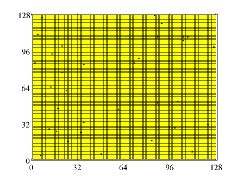
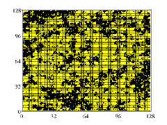
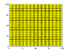
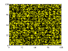
Figure 1: Snapshots of the spin configurations are given for two different concentrations $x$ of spin-1/2 and two different values of temperatures $T$. For $x=0.25$, $T=0.5$ (a) and $T=1.5$ (b); $x=0.75$, $T=0.5$ (c) and $T=1.5$ (d). spin-1/2 (spin-1) are represented by yellow (black). The temperature is measured in units of $J/k_{B}$.

We prepared the system with the spins randomly distributed on the lattice. The concentration $x$ of spin-1/2 and $(1-x)$ spin-1, is fixed. However, each spin-1/2 can have as its nearest-neighbor spins of the type spin-1/2 or spin-1 and vice versa. Each trial change of a spin state on the lattice is accepted according to the Metropolis prescription metropolis , $\omega(\alpha\rightarrow\alpha^{\prime})=\min[1,\exp(-\beta\Delta E)]$, where $\Delta E$ is the local energy change $(E_{\alpha^{\prime}}-E_{\alpha})$ resulting from changing the state of a random selected spin from $\alpha$ to $\alpha^{\prime}$ state, and $\beta=1/k_{B}T$. To reach the equilibrium state we take for guarantee at least $1\times 10^{6}$ MCs (Monte Carlo steps) for all the lattice sizes we studied. Then, we take more $5\times 10^{5}$ MCs to estimate the average values of the quantities of interest. Here, 1 MCs means $L^{2}$ trials to change the state of a spin of the lattice. The average over the disorder was done by using 100 independent samples for lattices in the range $12\leq L\leq 48$.

In Fig. 1, we have a snapshot of the concentrations of spin-1/2 and spin-1, and they were made for two different concentrations $x=0.25$ and $x=0.75$ of spin-1/2. In both cases, it has been analyzed the different concentrations at low temperatures ($T<T_{c}$, $T=0.5$) as shown in Fig. 1(a) and Fig. 1(c), and at high temperatures ($T>T_{c}$, $T=1.5$) as shown in Fig. 1(b) and Fig. 1(d). The temperature is measured in units of $J/k_{B}$ throughout the paper.

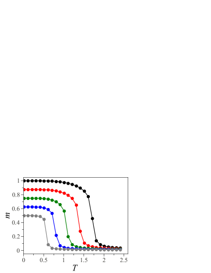
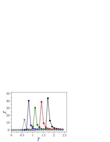
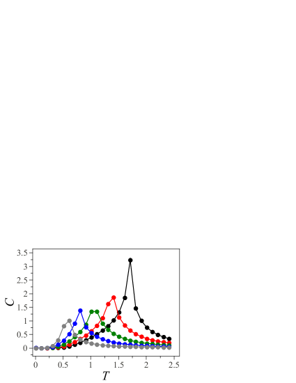
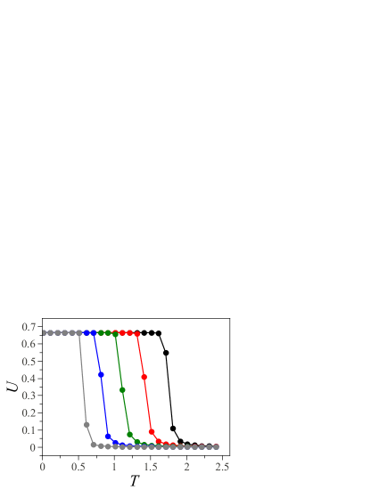
Figure 2: Thermodynamic quantities per site as a function of temperature $T$, and for several values of the concentration $x$ of spin-1/2. (a) Magnetization $m$, (b) susceptibility $\chi$, (c) specific heat $C$ and (d) fourth-order Binder cumulant $U$. The concentration $x$ of spin-1/2 is $x=1.0$ (gray line), $x=0.75$ (blue line), $x=0.50$ (green line) , $x=0.25$ (red line) and $x=0$ (black line). The temperature is measured in units of $J/k_{B}$.

All the results of the simulations presented here were realized for a concentration $x$ of spin-1/2 fixed at $x=$ 0, 0.25, 0.50, 0.75, 1.0. In Fig. 2, we displayed the behavior of the magnetization (Fig. 2(a)), susceptibility (Fig. 2(b)), specific heat (Fig. 2(c)) and fourth-order Binder cumulant (Fig. 2(d)) as a function of temperature $T$, and several values of the concentration $x$ of spin-1/2. For $x=0$, we have the critical behavior of the Blume-Capel model with the term of anisotropy equal zero $(D=0)$ blume ; capel . Nevertheless, for $x=1.0$, we have the case of the pure Ising model. The critical behavior for $x=0.5$0, i. e., half of the lattice with spin-1/2 and another half of the lattice with spin-1 randomly distributed were studied in the reference godoy . We can observe that the magnetization vanishes with the increase of temperature $T$. When the concentration $x$ of spin-1/2 increases $(x\rightarrow 1)$ the magnetization vanishes at different values of critical temperatures $T_{c}$. The critical temperature decreases with the increase of the concentration $x$ of spin-1/2. These can be clearly observed by the shifting in the susceptibility and specific heat peak (see Fig. 2(b) and 2(c)).

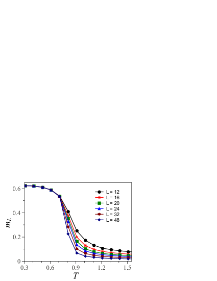
Figure 3: Magnetization $m_{L}$ as a function of temperature $T$ for various lattice sizes $L$ as indicated in the figure. The temperature is measured in units of $J/k_{B}$.

The finite-size effects of the magnetization were studied for the concentration $x$ of spin-1/2 fixed at $x=0.75$ and for various system sizes $L$. In Fig. 3, it is shown the behavior of the magnetization as a function of temperature $T$ for several system sizes $L$. We can observe in this figure, that the magnetization $m_{L}$ vanishes with the increase of temperature $T$, indicating the existence of a phase transition.

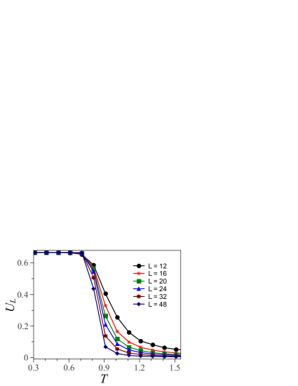
Figure 4: Fourth-order cumulants $U_{L}$ as a function of temperature $T$ for various lattice sizes $L$ as indicated in the figure. The temperature is measured in units of $J/k_{B}$.

So as to study the phase transition in more details, we used the fourth-order Binder cumulants $U_{L}$ intersection method to determine the value of temperature at which the transition occurs. According to the theory of finite-size scaling for continuous phase transitions, the finite-size behavior is governed by the ratio $L/\xi$, where $\xi$ is the correlation length. The scaling relation for the fourth-order cumulant shows that, at critical temperature, where the correlation length is infinite, all the curves must intercept themselves at a single point, since $L/\xi$ is zero for all the sizes $L$. To find the critical temperature, we displayed in Fig. 4 the cumulants $U_{L}(T)$ versus temperature $T$, for several system sizes $L$ and for $x=0.75$. Our estimate for the dimensionless critical temperature is $T_{c}=(0.71\pm 0.01)J/k_{B}$.

The susceptibility $\chi_{L}$ as a function of temperature $T$ is shown in Fig. 5. For finite systems $\chi_{L}$ presents a peak around the critical temperature $T_{c}$, which grows in height with the increase of the system size.

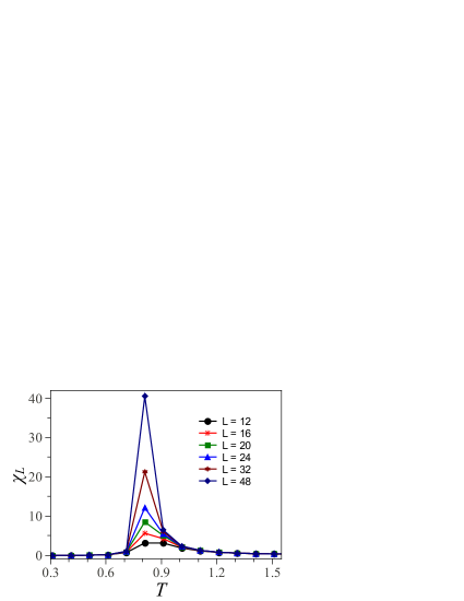
Figure 5: Susceptibility $\chi_{L}$ as a function of temperature $T$ for various lattice sizes $L$ as indicated in the figure. The temperature is measured in units of $J/k_{B}$.

In Fig. 6, we also present the measurements of the specific heat. The peak observed in the curves of the specific heat exhibit a weak system size dependence compared to the susceptibility peak. The position of the specific heat and of the susceptibility peaks can be defined at a pseudocritical temperature $T^{max}(L)$. The $T^{max}(L)$ approaches $T_{c}$ when $L\rightarrow\infty$ fisher .

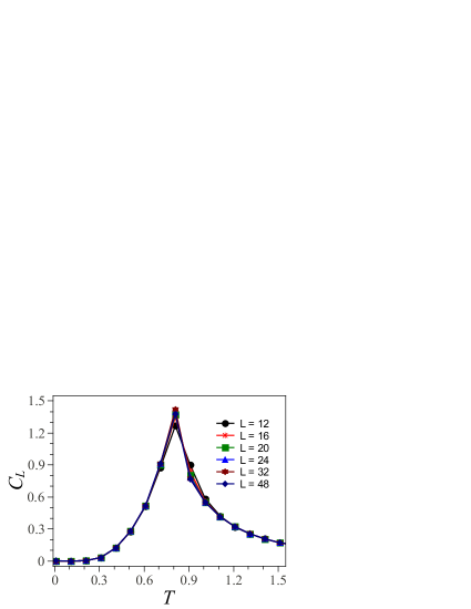
Figure 6: Specific heat $c_{L}$ as a function of temperature $T$ for various lattice sizes $L$ as indicated in the figure. The temperature is measured in units of $J/k_{B}$.

We have also calculated the critical temperature $T_{c}$ for several different values of the concentration $x$ of spin-1/2, as it can be seen in Fig. 7. For $x=0$ (only spin-1), we found $T_{c}=(1.69\pm 0.01)J/k_{B}$, that is the critical temperature of the Blume-Capel model with $D=0.0$. Yet, for $x=1.0$ (only spin-1/2), $T_{c}=(0.565\pm 0.003)4J/k_{B}$ which is the critical temperature of the Ising model. When $x=0.50$ (half of spin-1/2 and half of spin-1) the critical temperature is $T_{c}=(1.00\pm 0.003)J/k_{B}$ , therefore, the result is not according to the one of the referencegodoy . The general features of the phase diagram show that the critical temperature change when concentration varies $0<x<1.0$.

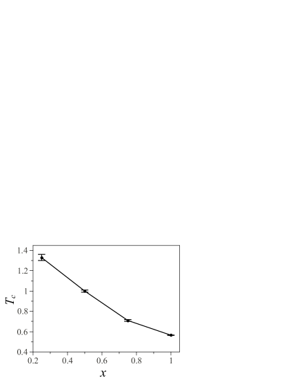
Figure 7: Critical temperatures $T_{c}$ as a function of the concentration $x$ of spin-1/2. The critical temperatures are measured in units of $J/k_{B}$.

IV Conclusions

We have studied a disordered ferromagnetic binary Ising model on a square lattice. The model consists of two different types of particles with spin-1/2 and spin-1. These particles are randomly distributed on the square lattice, and we considered only nearest-neighbor interactions. We also calculated the critical temperature $T_{c}$ for several different values of the concentration $x$ of spin-1/2. For $x=0$ (only spin-1), we found the critical temperature of the Blume-Capel model with $D=0.0$. On the other hand, for $x=1.0$ (only spin-1/2) we found the critical temperature of the Ising model. We have showed that the phase diagram present different critical temperatures for several values of the concentration $x$ of spin-1/2.

- (1) R. B. Stinchcombe in Phase Transitions and Critical Phenomena, edited by C. Dombo and J. L. Lebowitz (Academic, London, 1983), Vol. 7.
- (2) M. F. Thorpe and A. R. McGurn, Phys. Rev. B 20, 2142 (1979).
- (3) S. Katsura, Can. J. Phys. 52, 120 (1974).
- (4) T. Kaneyoshi, Phys. Rev. B 34, 7866 (1986).
- (5) P. D. Scholten, Phys. Rev. B 32, 345 (1985).
- (6) T. Kaneyoshi, Phys. Rev. B 33, 7688 (1986).
- (7) T. Kaneyoshi, Phys. Rev. B 39, 12134 (1989).
- (8) J. A. Plascak, Physica A 198, 655 (1993).
- (9) M. Godoy and W. Figueiredo, Int. J. Mod. Phys. C 20, 47 (2009).
- (10) K. Binder and D. W. Heermann, Monte Carlo Simulation in Statistical Physics. An Introduction, 3rd edn. (Springer, Berlin, 1997).
- (11) K. Binder in Finite-Size Scaling and Numerical Simulation of Statistical Systems, edited by V. Privman (World Scientific, Singapore, 1990) p. 173.
- (12) N. Metropolis, A. Rosenbluth, M. Rosenbluth, A. Teller and E. Teller, J. Chem. Phys. 21, 1087 (1953).
- (13) M. E. Fisher. Proceedings of the 51st Enrico Fermi Summer School, Varena, Italy, ed. M. S. Green, (Academic Press, New York, 1971).
- (14) 2 D.P. Belanger and A.P. Young, J. Magn. Magn. Mater. 100, 272 (1991).
- (15) M. Blume, Phys. Rev. 141, 517 (1966).
- (16) H. W. Capel, Physica 32, 966 (1966).