Magnetic clouds in the solar wind: A numerical assessment study of analytical models

Abstract

Context. Magnetic clouds (MCs) are “magnetized plasma clouds” moving in the solar wind. MCs transport magnetic flux and helicity away from the Sun. These structures are not stationary but feature temporal evolution as they propagate in the solar wind. Simplified analytical models are frequently used for the description of MCs, and fit certain observational data well.

Aims. The goal of the present study is to investigate numerically the validity of an analytical model which is widely used for the description of MCs, and to determine under which conditions this model’s implied assumptions cease to be valid.

Methods. A numerical approach is applied. Analytical solutions that have been derived in previous studies are implemented in a 3-D magnetohydrodynamic simulation code as initial conditions.

Results. Initially, the analytical model represents the main observational features of the MCs. However, these characteristics prevail only if the structure moves with a velocity close to the velocity of the background flow. In this case an MC’s evolution can quite accurately be described using an analytic, self-similar approach. The dynamics of the magnetic structures which move with a velocity significantly above or below that of the velocity of the solar wind is investigated in detail. Besides the standard case in which MCs only expand and propagate in the solar wind, the case of an MC rotating around its axis of symmetry is also considered, and the resulting influence on the MC’s dynamics is studied.

Conclusions. A comparison of the numerical results with observational data indicates reasonable agreement especially for the intermediate case, in which the MC’s bulk velocity and the velocity of the background flow are equal. In this particular case, analytical solutions obtained on the basis of a self-similar approach indeed describe the MC’s evolution quite accurately. In general, however, numerical simulations are necessary to investigate the evolution as a function of a wide range of the parameters which define the initial conditions.

1 Introduction

It is well-known that coronal mass ejections (CMEs) are one of the most significant forms of solar activity. They carry enormous masses of plasma, threaded by a magnetic field, away into the interplanetary medium. Further away from the Sun, these large-scale, dynamical plasma structures are commonly called interplanetary coronal mass ejections (ICMEs). A magnetic cloud (MC) is a specific type of ICME (see e.g. Burlaga 1995; Wimmer-Schweingruber et al. 2006; Démoulin et al. 2008) and can be considered as a magnetically isolated structure moving in the solar wind. Three features of such magnetic structures – an enhanced magnetic field, the rotation of this magnetic field and the low proton temperatures – are selected as bona fide signatures of MCs (Burlaga 1995). In situ observations of these physical properties of MCs are considered as important prerequisites towards a prediction of the geophysical effectiveness of their interaction with the Earth’s magnetosphere, i.e. for space weather forecasts and related issues.

Different models for the structures of MCs have been proposed. While there is no general agreement about their large-scale structure, the local structure of MCs is commonly considered in the form of cylindrically symmetric force-free configurations (Burlaga 1988, 1991; Démoulin & Dasso 2009). It is often suggested that the ends of MCs connect to the solar surface while, according to some other models, MCs are described as tori (Lacoste & Ouwehand 2006; Romashets et al. 2007). These models can be useful for capturing particular features of MCs, such as the curvature of an MC’s axis. In a number of studies, MCs are considered as force-free, static, axially symmetric rigid flux ropes and their magnetic field is constructed on the basis of Lundquist’s model (Burlaga 1988; Lepping et al. 1990; Farrugia et al. 1993). None of these analytical studies do consider interactions of MCs with the ambient environment. Observations show, however, that MCs do not stay static but expand while propagating in the solar wind, they keep expanding well beyond 1 AU, and they dynamically interact with the background solar wind flow (Burlaga 1991; Bothmer & Schwenn 1998; Démoulin et al. 2008; Démoulin & Dasso 2009).

Analytical models describing the features of MCs are used with remarkable success by a number of experts in order to describe certain observational data. Derivations of the analytical expressions for physical variables characterizing MCs are based on the assumption that a MC represents a self-similarly evolving cylindrical structure (Dalakishvili et al. 2011; Démoulin & Dasso 2009; Nakwacki et al. 2008; Farrugia et al. 1995a, 1993; Lepping et al. 1990; Burlaga 1988). We find it appropriate and necessary to numerically investigate the validity of such analytical models. For this purpose, it is seems reasonable to start out with a comparably simple model based on analytical considerations, and then to successively relax these simplifications towards more realistic configurations. This procedure is then able to reveal the extent to which simplifications such as the assumption of self-similarity maintain their validity in more complex settings.

Several numerical studies (de Sterck & Poedts 1999, 2000; Manchester et al. 2004; Chané et al. 2006; Dalakishvili et al. 2009) have been performed to explore character of magnetized plasma flows near MCs by treating them as superconductors, i.e. the magnetic field does not penetrate the cylindrical structure. Owens et al. (2005) have revealed that the region in front of an interplanetary MC has a rather complicated structure. In order to gain more insight into the characteristics of this region and the physical phenomena within it, and in order to better understand the geo-effectiveness of MCs, a refined investigation of MC dynamics is required.

For instance, it is to be expected (and has in fact been demonstrated numerically by, e.g. Odstrčil & Pizzo (1999) that variations in the structure of the background wind can severely distort the initially simple geometry of a MC. Furthermore, Riley & Crooker (2004) have used MHD simulations as well as kinematic arguments to show that MCs tend to flatten out as they propagate outwards, but still stress the paramount significance of force-free field models for the interpretation of MC observations. It is thus of vital importance to establish under which conditions (if any) these simple force-free models continue to be applicable. The need to eliminate all secondary effects to access the true net effect of a perturbing magnetic cloud on the ambient solar wind justifies our deliberate choice of both a cylindrical MC geometry and an unstructured background flow (see Section 3) as a first step towards this goal.

The existence of analytical models properly describing the evolution of MCs is very valuable for the field. Dalakishvili et al. (2011) numerically investigated the evolution of self-similar analytical solutions and showed that the solutions maintain a self-similar structure for a comparatively long time. However, in this 1-D study the entire structure was considered to be cylindrically symmetric, and it was assumed that the background solar wind could be described on the basis of a self-similar approach. In the present study we employ a 3-D code and implement a more general background flow.

In recent years, various numerical studies have been performed to investigate the initiation and the dynamics of CMEs (van der Holst et al. 2005, 2007; Jacobs et al. 2006; Kleimann et al. 2005, 2009; Aschwanden et al. 2008; Riley et al. 2008; Amari et al. 2010). These authors studied the initiation and propagation of solar eruptions in the heliosphere, and followed the evolution of magnetic structures in a 3-D setting. The numerical solutions show that far from the Sun, the steady-state solar wind can be characterized by a radial velocity and, to some approximation, by a radial magnetic field. Therefore, in our simulations we employed a radial flow with a radial magnetic field as an initial background in order to study the evolution of MCs at larger heliocentric distances. The diameter of the MC is only 0.2 AU at 1 AU, so we could assume the physical characteristics of the ambient solar wind not to change significantly in the region where it interacts with the MC.

Additionally, since a rotation of MCs about its axis of symmetry is deduced from observations (Burlaga 1995; Farrugia et al. 1995b; Klein & Burlaga 1982), we found it necessary to start an investigation of the dynamics of MCs taking into account this rotation. This is possible by analytically formulating an appropriate initial set-up. As stated above, many groups have simulated MCs, and various tests and comparisons of numerical models with each other and with measurements have been performed, see, e.g. Vandas et al. (2010, 2009) and reference therein. It appears, however, that comprehensive, systematic comparisons of analytical models of MCs with their full three-dimensional numerical simulations have not been made – there are only a few studies into this direction. For example, Vandas & Odstrčil (2000) have compared the analytical model by Osherovich et al. (1995) with two-dimensional numerical simulations and found very good agreement. Although the analytical model served mainly as a test case for the numerical simulations, Vandas & Odstrčil (2000) came to the conclusion that the analytically determined asymptotic behavior of the magnetic field on the axis of an expanding flux tube has a rather general validity.

Other authors have compared numerical and analytical results of certain aspects of MC physics, see e.g. Xiong et al. (2006), who studied the geo-effectiveness of so-called shock-overtaking MCs with a 2.5-dimensional model. More recently, Taubenschuss et al. (2010) have also performed 2.5-dimensional simulations and compared them regarding the expansion speed to some extent with analytical findings by Owens et al. (2005), resulting in average agreement. Interestingly, these authors also claim that their simulations reveal that the force-free configuration for MCs seems to be conserved very well, at least when averaging over the entire cross section.

With the present analysis, we compare a recently developed analytical model with three-dimensional numerical simulations. The remainder of this paper is organized as follows: in Section 2 we describe the analytical and in Section 3 the numerical model, including the implemented initial and boundary conditions. In Section 4 we describe details of the simulation setup. In Section 5, the results of our simulations are presented and discussed, and in Section 6 we summarize the results of our work and discuss the conclusions as well as indicate future plans.

2 Analytical background

In this section we briefly summarize the analytical model developed in Dalakishvili et al. (2011). To perform an analytic study of the dynamics of magnetic clouds, we have to start from the full set of ideal MHD equations

$$\nabla\cdot\@vec{B} =0,$$ (1)

$$\partial_{t}\@vec{B} =\nabla\times\left[\@vec{V}\times\@vec{B}\right]$$ (2)

$$\partial_{t}\varrho+\nabla\cdot\left(\varrho\@vec{V}\right) =0$$ (3)

$$\varrho\left[\partial_{t}+\left(\@vec{V}\cdot\nabla\right)\right]\@vec{V} =\mu^{-1}(\nabla\times\@vec{B})\times\@vec{B}-\nabla p$$ (4)

In these equations, $p$ denotes the thermal plasma pressure, $\varrho$ is the mass density, $\@vec{V}$ is the velocity field, $\@vec{B}$ denotes the magnetic field, and $\mu$ is the permeability of free space.
The problem is considered in the frame of the MC and in cylindrical coordinates centered on the MC, i.e. with a longitudinal axis $z$ that coincides with the MC’s axis. In a number of previous studies, the MCs were considered as cylindrical magnetic structures, characterized by axial symmetry. In the present consideration, both symmetry along the $z$ axis ($\partial_{z}=0$) and the azimuthal direction ($\partial_{\varphi}=0$) are assumed. The axially symmetric magnetic field can then be expressed as

$$\@vec{B}\equiv[\ 0,\ B_{\varphi},\ B_{z}]$$ (5)

where $B_{\varphi}=B_{\varphi}(r,t)$ and $B_{z}=B_{z}(r,t)$. We note that this representation satisfies the solenoidal condition (1).
The self-similar approach, adopted here, implies that the temporal evolution of the physical functions is controlled by the self-similarity variable

$$\xi\equiv\frac{r}{\Phi(t)}$$ (6)

where $\Phi(t)$ is a function of time. In analogy to Low (1982), let us search solutions of the MHD equations in the following form:

$$B_{\varphi} =\Phi^{\delta}Q_{\varphi}(\xi)$$ (7a)

$$B_{z} =\Phi^{\sigma}Q_{z}(\xi)$$ (7b)

$$\varrho =\Phi^{\alpha}\tilde{\rho}(\xi)$$ (7c)

$$p =\Phi^{\beta}\tilde{p}(\xi)$$ (7d)

One can see that the type of solutions introduced by Eqs. (7a-7d) evolve self-similarly and are characterized by a particular time-scaling. Here $Q_{\varphi}$, $Q_{z}$, $\tilde{\rho}$, and $\tilde{p}$ are functions of the self-similar variable $\xi$, and $\Phi^{\delta}$, $\Phi^{\sigma}$, $\Phi^{\alpha}$, and $\Phi^{\beta}$ show the time scaling of the azimuthal and longitudinal components of the magnetic field, the plasma density, and the plasma pressure, respectively.
We consider both a radial and a longitudinal expansion of the MC, but no motion in the azimuthal direction. In this case, the Eulerian velocity field of the plasma, $\@vec{V}$, can be expressed as

$$\@vec{V}=\left[V_{r},\ 0,\ V_{z}\right],$$ (8)

where we assume that the radial component of the velocity $V_{r}=V_{r}(r,t)$, and the $z$ component $V_{z}=V_{z}(z,t)$, i.e. we assume that the MC maintains its cylindrical shape during its evolution.
The solutions readily follow from the derived equations (see Dalakishvili et al. 2011), yielding

$$\@vec{V}_{r,\varphi,z} =\frac{k}{1+kt}\left[r,0,z\right]$$ (9a)

$$\varrho =\frac{\tilde{\varrho}}{(1+kt)^{3}}$$ (9b)

$$p =\frac{\tilde{p}}{(1+kt)^{4}}$$ (9c)

where $\tilde{\varrho}$ and $\tilde{p}$ are arbitrary functions of $\xi=r/\Phi$. The components of the magnetic field read

$$\@vec{B}_{r\varphi z}=\frac{B_{0}}{(1+kt)^{2}}\left[\ 0,\ J_{1}\left(\frac{r}{\tilde{r}_{0}(1+kt)}\right),\ J_{0}\left(\frac{r}{\tilde{r}_{0}(1+kt)}\right)\right],$$ (10)

where $J_{0}(x)$ and $J_{1}(x)$ are the Bessel functions of the first kind while $B_{0}$ and $\tilde{r}_{0}$ are constants. Here $k$ is a constant parameter and $1/k$ has unit of time and characterizes the MC’s rate of radial expansion.

3 Description of the model

3.1 Coordinate systems

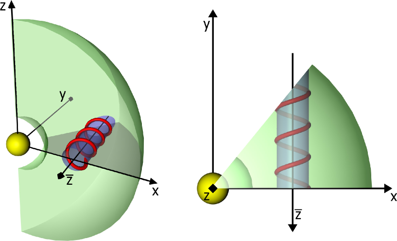
Figure 11: Sketch of the computational volume with the global, Sun-centered $(x,y,z)$ system, and the MC (cylinder with $\bar{z}$ axis and exemplary field lines) in the ecliptic plane.

It is assumed that an MC is initially a cylindrical structure placed in the radial solar wind flow. The MC’s initial bulk velocity is perpendicular to its axis of symmetry. Hereafter, in order to formulate the initial conditions with particular expressions in a compact way, we introduce local and global coordinate systems. The global coordinate system which we use is a spherical one $(R,\vartheta,\varphi)$ centered on the Sun. The polar axis of this system coincides with the solar magnetic axis (the $z$ axis), and the azimuthal angle $\varphi$ is counted from the $x$ axis, which is directed from the Sun to the Earth. The local, cylindrical coordinate system ($r,\tilde{\varphi},\tilde{z}$) is related to a cylindrical magnetic cloud: the $\tilde{z}$ axis coincides with the axis of the MC and is perpendicular to the $(x,z)$ plane, such that $(x,z,\tilde{z})$ defines a right-handed Cartesian coordinate system. The azimuthal angle of the local system $\tilde{\varphi}$ is counted from the $z$ axis of the global system. Fig. 11 shows a sketch of the computational volume and the respective coordinate axes. After fixing the location of the cylinder in the global system, we can define functional relations between the coordinates of these two systems and transform vector components from one system to another. Later, the notation $C_{r,\tilde{\varphi},\tilde{z}}$ will indicate components of a vector $\@vec{C}$ in the local coordinate system, while $C_{R,\vartheta,\varphi}$ will denote the components of the same vector in the global coordinate system.

3.2 Initial and boundary conditions

The physical quantities are normalized as follows. The unit length $L_{0}=7\cdot 10^{5}$ km is equal to the Solar radius. The unit magnetic field $B_{0}=3$ nT, unit number density $n_{0}=10$ cm^-3, and mass density $\rho_{0}=m_{\rm p}n_{0}=1.7\cdot 10^{-20}$ kg/m³ (where $m_{\rm p}$ is the proton mass) approximate their respective values at 1 AU. The speed is then normalized to $V_{\rm 0A}=B_{0}/\sqrt{\mu\rho_{0}}=20.5$ km/s (i.e. of the order of the MC’s expansion velocity in the local frame, according to Vandas et al. (2009)) and, finally, the unit of time is then given by $t_{0}=L_{0}/V_{0A}=9.5$ h. As a background plasma flow at large heliocentric distances we consider a radial flow with a radial magnetic field. In order to ensure the stationarity of this background flow, we choose the following expressions for the initial background density and radial magnetic field:

$$\varrho_{\rm out} =\varrho_{0,{\rm out}}\left(\frac{1}{R}\right)^{2}$$ (11a)

$$B_{{\rm out},R,\vartheta,\varphi} =B_{0,{\rm out}}\left(\frac{1}{R}\right)^{2}\left[\Theta(\vartheta),0,\ 0\right].$$ (11b)

Here $\Theta(\vartheta)$ is an arbitrary

function of the polar angle. In our simulations, we considered both the case $\Theta(\vartheta)=1$ and $\Theta(\vartheta)=\cos\vartheta$. The latter case describes the change of sign of the magnetic field and the existence of a current sheet in the equatorial plane. We found that such asymmetry in the magnetic field does not have a significant influence on the dynamics of the MC. Inside the MC, the force-free magnetic fields of Eq. (10), evaluated at $t=0$, is superimposed on background radial field:

$$\@vec{B}_{\rm in}=\@vec{B}_{\rm in}^{\prime}+\@vec{B}_{\rm out}\ .$$ (12)

In the local coordinate system, the former becomes

$$\@vec{B}_{{\rm in}\ r,\tilde{\varphi},\tilde{z}}^{\prime}=B_{0,{\rm in}}\left[0,\ J_{1}\left(\frac{r}{\tilde{r_{0}}}\right),\ J_{0}\left(\frac{r}{\tilde{r_{0}}}\right)\right]\ .$$ (13)

We note that Eq. (13) coincides with Lundquist’s solution (Lundquist 1950).
Here, $\tilde{r_{0}}$ is a same arbitrary constant parameter introduced in Eq. (10). In the numerical simulations, $\tilde{r_{0}}$ is equal to the MC’s initial radius. For a determination of the constants $B_{0,{\rm in}}$ and $B_{0{\rm out}}$, the observational data, which show that the plasma beta inside a MC is lower than outside ($\beta_{\rm in}\ll 1$, $\beta_{\rm out}\sim 1$) (Burlaga et al. 1981; Burlaga 1991; Bothmer & Schwenn 1998) were taken into consideration.

The evolution of an MC is characterized by an increase of its radial and longitudinal extent, and by the translational and rotational motion of the whole structure in the ambient environment. The velocity of matter inside the MC consists of the MC’s bulk velocity (which is initially perpendicular to the MC’s axis of symmetry), the velocity caused by an increase of its radius, and the velocity of lengthening. Substituting $t=0$ in Eq. (9a), we derive the expressions for the components of the velocity inside the MC

$$\@vec{V}_{{\rm in}\ r,\tilde{\varphi},\tilde{z}}^{\prime}=k\left[r,\ 0,\ \tilde{z}\right].$$ (14a)

given in the coordinate system attached to the MC. The total velocity of matter inside the MC is then

$$\@vec{V}_{\rm in}=\@vec{V}_{\rm MC}+\@vec{V}_{\rm in}^{\prime}\ .$$ (14b)

The initial background velocity is prescribed to be radial and constant far away from the MC, and tangential to the MC’s surface, i.e. the background plasma does not penetrate the MC. An expression for the velocity which satisfies the above-mentioned conditions is:

$$\@vec{V}_{\rm out}=\@vec{V}+\@vec{V}^{\prime}\ .$$ (15a)

where

$$\@vec{V}=(V_{R},0,0)$$ (15b)

in the global coordinate system. It is convenient to express $\@vec{V}^{\prime}$ in local cylindrical coordinates:

$$V^{\prime}_{r} =\left(V_{S}+V_{{\rm MC},r}-V_{r}\right)\left(\frac{r_{0}}{r}\right)^{3}$$ (16a)

$$V^{\prime}_{\tilde{\varphi}} =\left(V_{{\rm MC},\tilde{\varphi}}-V_{\tilde{\varphi}}\right)\left(\frac{r_{0}}{r}\right)^{3}$$ (16b)

$$V^{\prime}_{\tilde{z}} =V_{{\rm MC},\tilde{z}}\left(\frac{r_{0}}{r}\right)^{3}\ .$$ (16c)

Here $V_{S}=kr_{0}$ is the initial Lagrangian velocity of the MC’s edge. The parameter $k$ is the constant introduced in Eq. (9a), see also Dalakishvili et al. (2011). Initially, the density inside the MC is uniform and half the unit density. The initial radius of the MC is 20 in normalized units, which corresponds to a value of 0.1 AU, which is confirmed to be reasonable by in-situ measurements (Burlaga 1995).
In addition to the kinematic case described by Eqs. (14a-16c), we also consider the interesting case in which the MC rotates around its axis. In this case we change Eq. (14a) and Eq. (16b) as follows:

$$V^{\prime}_{{\rm in},\tilde{\varphi}} =\omega r$$ (17a)

$$V^{\prime}_{\tilde{\varphi}} =\left(\tilde{V}_{{\rm MC},\tilde{\varphi}}-\tilde{V}_{\tilde{\varphi}}+\omega r\right)\left(\frac{r_{0}}{r}\right)^{3}\ .$$ (17b)

Here $\omega$ is the angular velocity of the MC’s rigid rotation around its symmetry axis.

We applied the following boundary conditions formulated in the global coordinate system: on the inner radial boundary we prescribe for the magnetic field and density the functions given by Eqs. (11a-11b) and a radially uniform velocity. On the other (opposite and other) boundaries, the density, the tangential components of the magnetic field, and the velocity are extrapolated, while for the normal components of the velocity and magnetic field we use mass and magnetic flux conservation conditions. One should bear in mind that the outer radial boundary conditions (whose choice was motivated by simplicity) are incompatible with the cylindrical geometry prescribed to the MC. While in principle one could expect an influence of these boundary conditions on the solutions, they turn out to be negligible far from the boundary: the propagation speed of the magnetic structures is the local Alfvén speed. Therefore, we could conclude that the boundary-induced disturbances will not be able to propagate inwards against the supersonic outflow.

3.3 Model equations and their implementation in the code

In order to study the dynamics of MCs numerically, we use a second-order finite volume scheme based on the work by Kurganov et al. (2001) for the hyperbolic part of the system of equations (1-4), see also Flaig et al. (2009) and references therein. This is a central conservative scheme for the solution of equations of type $\partial_{t}\@vec{u}+\nabla\cdot[\@vec{F(u)}]=\@vec{0}$. In our study we solve the following (normalized) equations:

$$\partial_{t}\rho+\nabla\cdot(\rho\@vec{V}) =0$$ (18a)

$$\partial_{t}(\rho\@vec{V})+\nabla\cdot\left[\rho\@vec{VV}+\left(p+B^{2}\right)\@tens{I}-\@vec{BB}\right] =0$$ (18b)

$$\partial_{t}\@vec{B}+\nabla\cdot(\@vec{VB}-\@vec{BV}) =0\ .$$ (18c)

The system is closed using the ideal gas

equation of state $p=\rho T$. The employed numerical scheme require neither a Riemann solver nor a characteristic decomposition, and was extended by means of a constrained transport description for the magnetic field (see, e.g., Balsara & Spicer 1999; Londrillo & Del Zanna 2000), which ensures the solenoidality of the magnetic field. This method uses the hyperbolic fluxes to compute the electric field components on a staggered grid. These are then used to evolve the magnetic induction, the components of which are also given on a (different) staggered grid. The stability of the code and its capability to resolve steep gradients without introducing spurious oscillations have been demonstrated, e.g. by Kissmann (2006) and Flaig et al. (2009).

In the employed code, the initial magnetic field is formulated by means of a vector potential. The vector potential whose curl results in the magnetic field of expression (13) can be expressed as

$$\@vec{A}_{{\rm in}\ r,\tilde{\varphi},\tilde{z}}^{\prime}=B_{0,{\rm in}}\left[0,\ J_{1}\left(\frac{r}{\tilde{r_{0}}}\right),\ J_{0}\left(\frac{r}{\tilde{r_{0}}}\right)\right]\ .$$ (19)

The vector potential corresponding to a radial magnetic field can be expressed in the global spherical coordinates as

$$\@vec{A}_{1R,\vartheta,\varphi}=\left[0,\ -\frac{B_{0\ {\rm out}}\Theta(\vartheta)\sin\vartheta}{R}\varphi,\ 0\right]\ .$$ (20)

In order to ensure continuity of the vector potential across the surface of the MC, we represent the vector-potential of the background magnetic field as

$$\@vec{A}_{\rm out}=\@vec{A}_{1}+\nabla f$$ (21)

with

$$f=B_{0{\rm in}}\left[r\left(1+\left(\frac{r_{0}}{r}\right)^{2}\right)+\tilde{r}_{0}J_{1}\left(\frac{r}{\tilde{r_{0}}}\right)\tilde{\varphi}+\tilde{r}_{0}J_{0}\left(\frac{r}{\tilde{r_{0}}}\right)\tilde{z}\right]\ .$$ (22)

while the vector potential of the MC’s magnetic field is given by

$$\@vec{A}_{\rm in}=\@vec{A}_{\rm in}^{\prime}+\@vec{A}_{\rm out}\ .$$ (23)

4 Details of the simulation setup

In this section, we present details of the performed simulations. The computational domain is a segment of a sphere bounded by $R\in[60,300]$, $\vartheta\in[0.1,0.9]\pi$, and $\varphi\in[0,0.2]\pi$. For the simulations we used 120 grid cells in the radial and polar dimensions and 60 cells in the azimuthal direction.
The initial velocity of the background flow is $V_{R}=20$, corresponding to $410$ km/s. The center of the cylindrical MC is initially located at $R_{0}=170$ and the MC’s initial radial size is $r_{0}=20$, with parameter $\tilde{r}_{0}=20$. We conducted various simulation runs, which are summarized in Table 1.

Table 1: Summary of conducted simulation runs, with references to the figures which display selected data from the respective runs.

Run	$V_{0}$	$\omega$	$B_{0out}$	Figures
1	15	0	$(200/R)^{2}$	1, 6
2	20	0	$(200/R)^{2}$	2, 3, 4
3	30	0	$(200/R)^{2}$	5, 6
4	20	0.05	$(200/R)^{2}$	9

In runs 1 to 3, we considered cases in which the MC’s bulk velocity $V_{0}$ is initialized to be lower than, equal to, or higher than the ambient flow speed of 20. Furthermore, the (formerly vanishing) MC’s internal rotation around its axis of symmetry was varied, as was the direction of the background B field (run 4). In all runs, the mass density inside the MC was $\rho_{\rm in}=0.5$ and the density outside the MC was $\rho_{\rm out}=(200/)R^{2}$. In order to describe the magnetic field inside the MC, we set the value of $B_{0,{\rm in}}=5$. The Lagrangian velocity of the MC’s edge is $V_{\rm S}=kr_{0}$ with $k=0.05$.

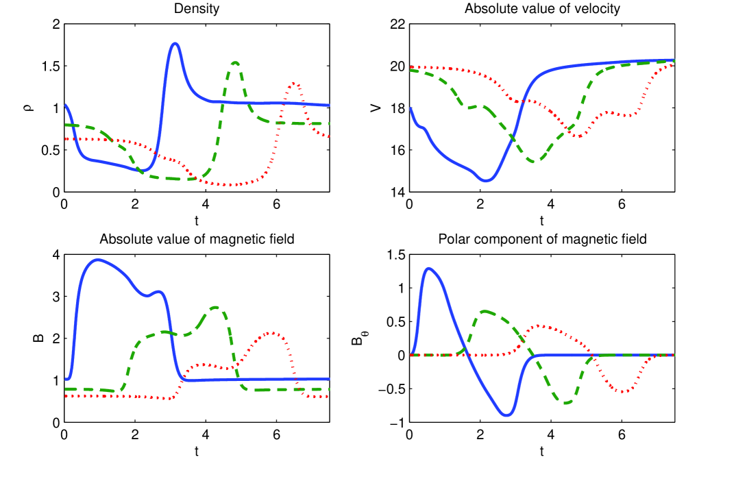
Figure 1: Plots of normalized density, velocity, total magnetic field, and polar component of the magnetic field. The solid, dashed, and dotted lines show the values recorded by virtual observers placed at $R=196$, $R=225$, and $R=250$, respectively. These plots correspond to run 1 (see Table 1), for which $V_{0}=15$ and $\omega=0$.

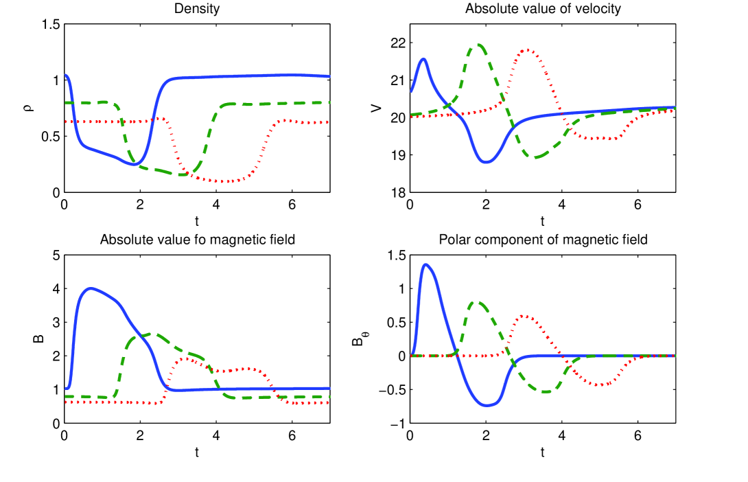
Figure 3: The same type of data as displayed as Fig. 1, here for run 2, when the MC’s initial velocity is $V_{0}=20$ (i.e. equal to that of the ambient wind). We see that the structure maintains the MC’s signatures during its evolution fairly well.

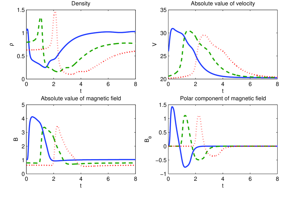
Figure 7: The same type of data as displayed in Fig. 1, here for run 3, when the MC’s initial velocity is $V_{0}=30$ (i.e. higher than that of the background wind).

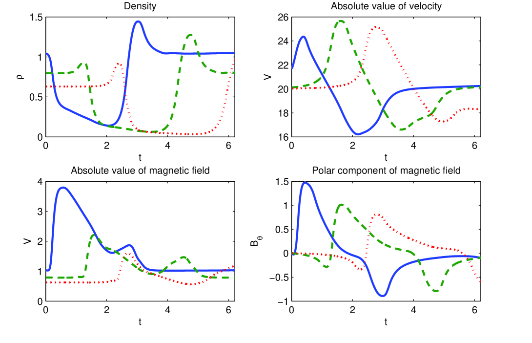
Figure 10: The same type of data display as Fig. 1 for run 4 ($V_{0}=20$, $\omega=0.05$).

In order to ease a comparison with observations as well as with analytical models, time profiles of density, magnetic field magnitude, and flow velocity at selected fixed positions along the MC’s trajectory have been extracted from the simulation data and presented in Figs. 1, 3, 7, and 10. These ”virtual observers” thus capture information which would be measured by a stationary spacecraft situated on the MC’s trajectory as the latter sweeps over it. All three “virtual observers” have the same polar and azimuthal coordinates, viz. $\vartheta^{\prime}=0.5\pi$ and $\varphi^{\prime}=0.03\pi$, and the respective distances of each of the three observers from the Sun are $R_{1}^{\prime}=196$, $R_{2}^{\prime}=225$, and $R_{3}^{\prime}=250$.

5 Results and discussion

5.1 Non-rotating MCs

In this section, we present and discuss the results of the numerical simulations described in the previous section.

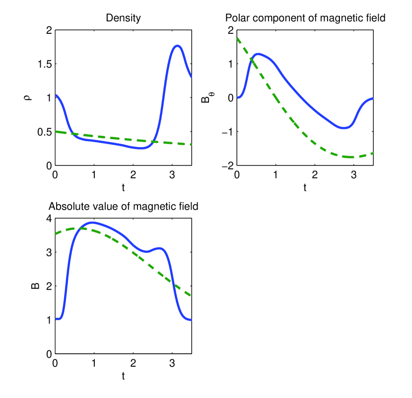
Figure 2: Plots of density, polar component of magnetic field, and absolute value of the magnetic field. The solid lines correspond to the values detected by a virtual observer situated at $R=196$. The dashed line shows values obtained using the analytical solution. The initial bulk velocity of the MC is $V_{0}=15$, its initial radius is $r_{0}=20$.

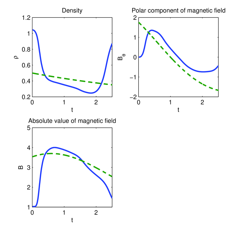
Figure 4: The same plot as in Fig. 2 but here for the case in which the MC’s velocity is $V_{0}=20$ (i.e. equal to that of the background wind).

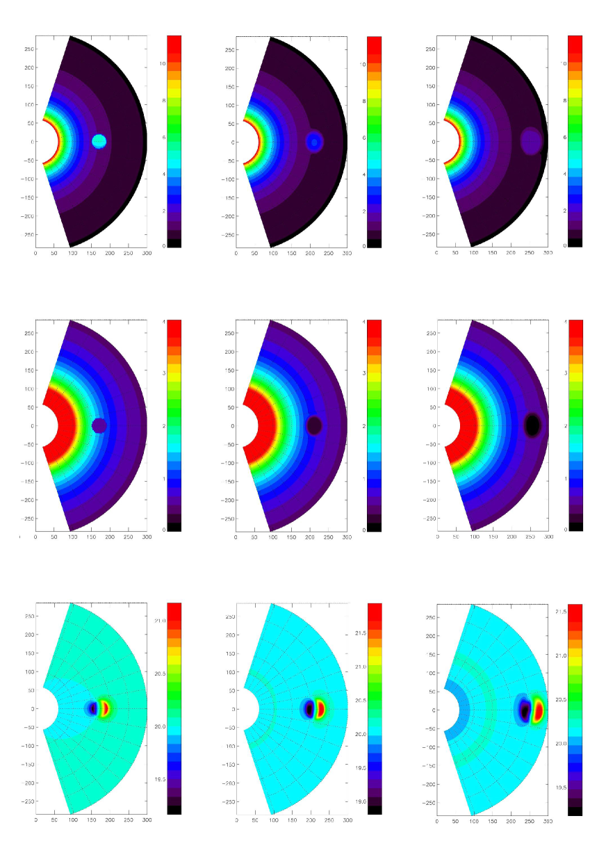
Figure 5: Cuts along the meridional plane $\varphi=0.03\pi$ for run 2 (see Table 1), displaying snapshots for the normalized values of the absolute magnetic field (top row), mass density (middle row), and absolute velocity (bottom row) at times $t=0$ (left column), $t=2$ (middle column), and $t=4$ (right column). The MC’s initial velocity is $V_{0}=20$ (i.e. equal to that of the background wind). The MC expands approximately symmetrically.

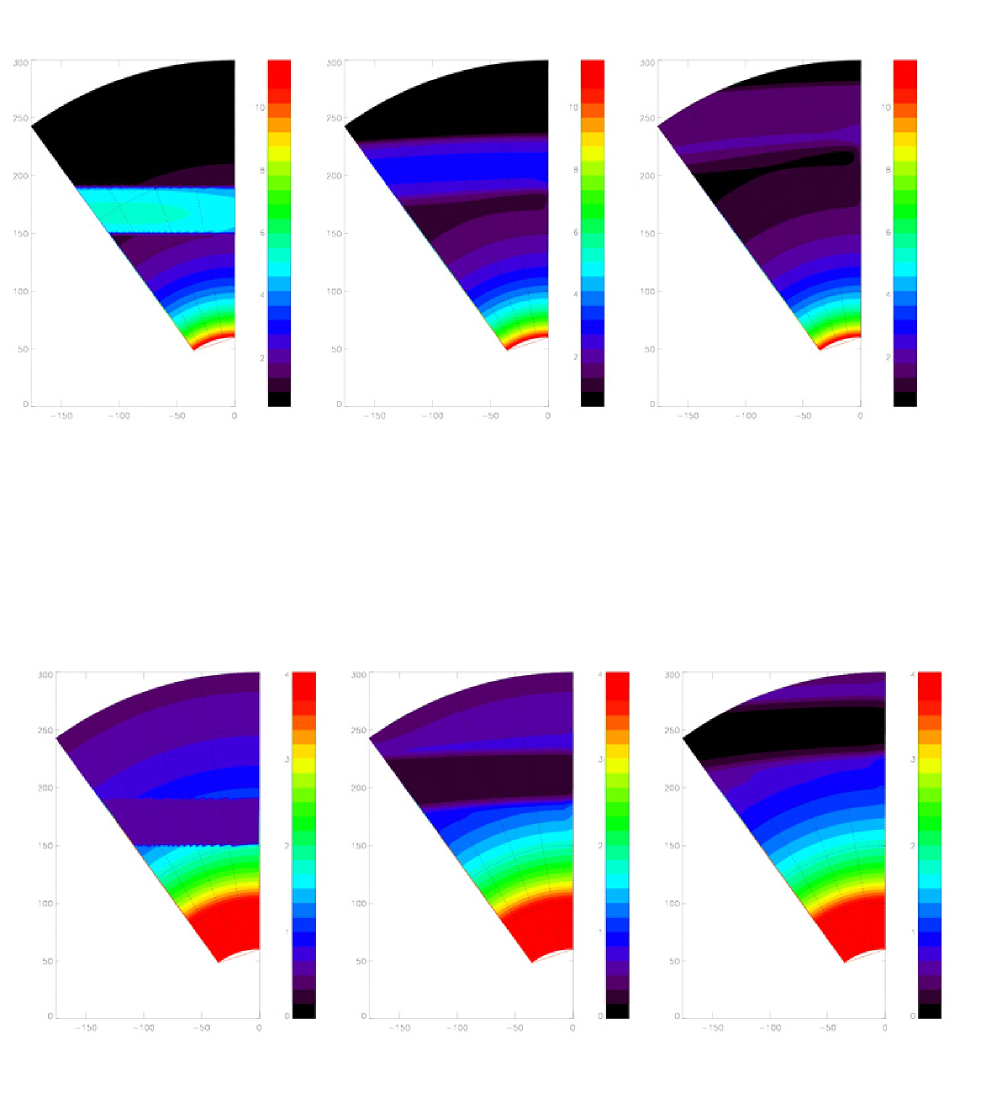
Figure 6: The same situation as depicted in Fig. 3 (run 2, $V_{0}=20$, $\omega=0$), except a cut in the equatorial plane is shown. Top row corresponds to the global structure of the magnetic field and bottom row shows global structure of mass density.

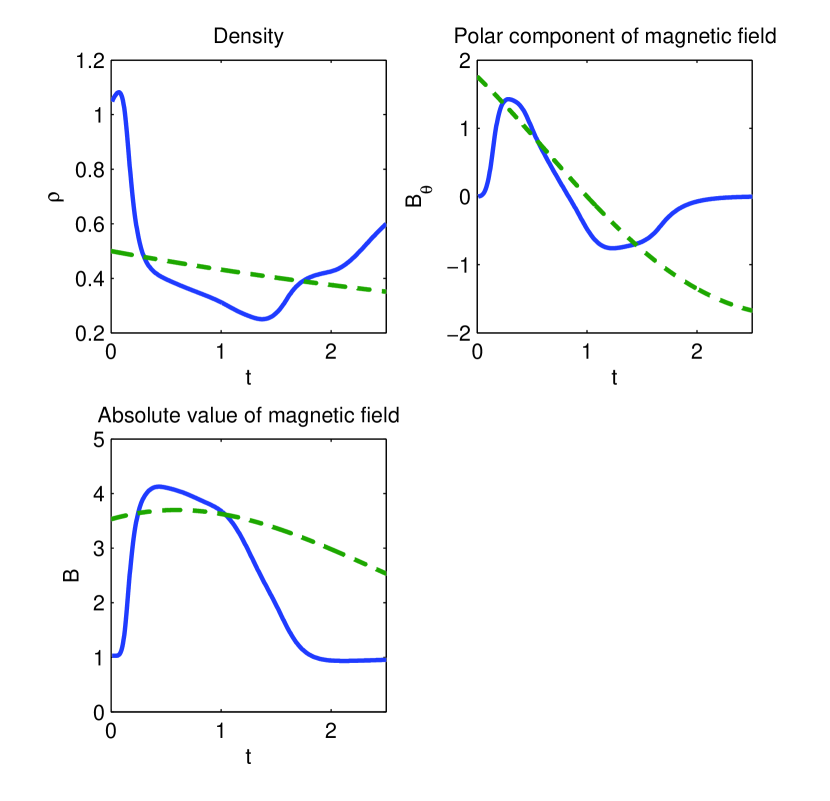
Figure 8: The same plot as in Fig. 2 but here for the case in which the MC’s initial velocity is $V_{0}=30$ and its initial radius is $r_{0}=20$.

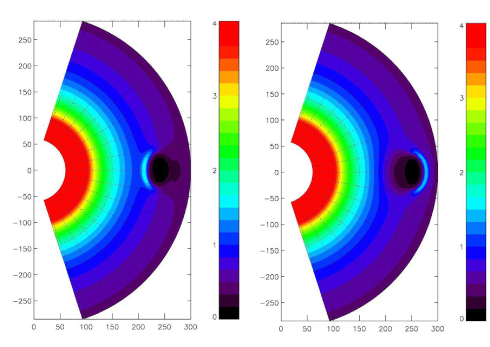
Figure 9: Density cuts along the meridional plane at time $t=2$ for run 1 (left panel) and run 3 (right panel). In the left panel the MC initially moves with velocity $V_{0}=15$ (i.e. slower than the background wind). The right panel corresponds to the case in which the MC initially moves with velocity $V_{0}=30$ (i.e. faster than the background wind). We see that the slow MC is followed by a denser region while the fast MC is preceded by a region with a sharp density gradient.

Figs. 1, 3, and 7 show time profiles of normalized density, velocity, total magnetic field, and polar component of the magnetic field for the runs 1 to 3 as given in Table 1 as recorded by the virtual observers. In Figs. 2, 4, and 8, these numerical results are compared with those obtained with the analytical model for the region inside the MC, i.e. the physical variables are plotted for the time interval from $t_{\rm in}$ when the observer situated at $R=196$ enters the MC until $t_{fin}$, when this observer leaves the MC again. $t_{in}$ and $t_{fin}$ are calculated analytically. These comparisons reveal that the analytical model describes the evolution of magnetic structures best for the case in which the MC initially moves with the velocity of the ambient solar wind. Fig. 5 provides plots of the global structure of the total magnetic field, mass density, and plasma velocity in a meridional plane ($\varphi={\rm const}$) and on Fig. 6 are shown structures of magnetic field and mass density in the equatorial plane. While these figures display the results for run 2, Fig. 9 shows the global structure of the number density in the meridional plane for runs 1 and 3. From the results shown in Figs. 5 and 6 we can conclude that when the velocity of the MC is close to the velocity of the background flow, the MC expands smoothly, i.e. although it does not maintain an exactly cylindrical shape (Fig. 5) and exhibits a slightly changing axis curvature (Fig. 6), the plasma density inside the MC decreases without developing strong gradients. Fig. 9 reveals that when the MC’s velocity is less than the velocity of the background flow, i.e. when the MC moves slower than the background solar wind, a denser region appears behind the MC after some time, while the MC which initially moves faster than the ambient solar wind is preceded by a region with a sharp (positive) density gradient. Observations do indeed show that MCs moving faster than the ambient solar wind are preceded by density enhancements (Klein & Burlaga 1982). The simulation results also show that the MC exhibits stronger deviations from a cylindrical shape as compared to the case shown in Figs. 5 and 6. From a comparison of the upper left and bottom left panels of Fig. 1 (density and absolute value of the magnetic field), one can see that after some time the observers detect an increase of magnetic field and density at about the same time (see dashed and dotted lines). Such structures that are characterized by sharp gradient of density can also be found in observational data, see (Lepping et al. 1997). We could conclude that – besides other factors such as a possible overtaking of slow clouds by fast corotating streams (Klein & Burlaga 1982) – dynamical processes occurring during the interaction of an MC with the ambient solar wind could play a crucial role for the creation of sharp density gradients in the vicinity of an MC. We also can see that the profile of the magnetic field strength evolves asymmetrically, which could be explained by the fact that the MC expands and, while an observer crosses this structure, the magnetic field inside the MC does not stay constant, but decreases in time. Note that very similar features are present in real observations, as exemplified in (Lepping et al. 1997). We can also see that due to an increase of the MC’s radius, the front parts of the MC are observed to propagate with a higher velocity than its rear regions. This feature is also observed in real data (e.g. Nakwacki et al. 2008).

From these results it is obvious that initially, in all three cases, an observer would detect the following main signatures of a magnetic cloud: 1) a decrease of the plasma density, 2) an increase of the magnetic field strength, and 3) a rotation of the magnetic field inside the MC. We see that during the evolution not all magnetic structures exhibit these main features. As a matter of fact, in the cases when the velocity of the magnetic structure differs much from the velocity of the background flow, the regions of lower density and higher magnetic field evolve differently in time, see Figs. 1 and 7. Only those structures that move with a velocity close to that of the background flow maintain the above-mentioned characteristic signatures.

5.2 Rotating MCs

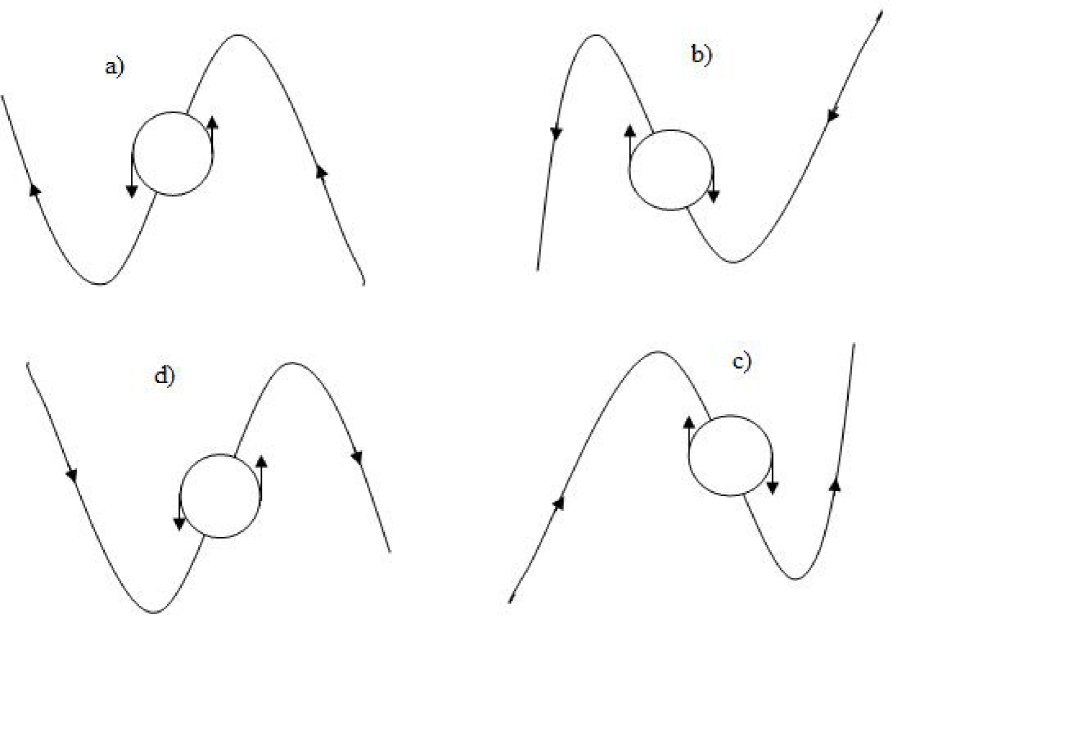
Figure 12: Illustration of the bending of a magnetic field line due to the rotation of the flux rope. Here it is assumed that solar wind flows from right to left. Panels a) and d) correspond to the north-south rotation of an MC, while panels b) and c) demonstrate the case of south-north rotation. Due to the MC’s rotation field lines of the background magnetic field are curved.

Fig. 10 shows the MC properties for the case in which the rotation of the MC around its axis of symmetry $\tilde{z}$, (see Fig.11) is taken into account. In Fig. 10 this is done for the case in which the background magnetic field direction coincides with the direction of the solar wind velocity and the MC rotates in the north-south direction (see panel a in Fig. 12). In Fig. 10, peaks of density and magnetic field one be discerned both in front of and at the rear of the MC. This can be understood as follows: A rotating MC generates a centrifugal force, which induces centrifugal motion of matter. One could thus expect an accumulation of mass at the edges of the MC and, due to the frozen-in condition, the magnetic field also moves and accumulates with the plasma. In the panel showing the polar component $B_{\vartheta}$ of the magnetic field, we can see that the rotation causes a bending of the ambient magnetic field lines. For instance, in the case of a north-south rotation and when the background magnetic field direction coincides with the direction of solar wind velocity, $B_{\vartheta}$ becomes negative in front of the MC, (See the bottom right panel in Fig. 10 and panel a in Fig. 12).

6 Summary and conclusions

In order to study the dynamics of MCs propagating in the solar wind, we numerically implemented analytical expressions for the physical variables characterizing an MC as initial conditions. These expressions were derived for self-similarly evolving MCs and introduced in a number of previous studies (Burlaga 1988; Lepping et al. 1990; Farrugia et al. 1993, 1995a; Nakwacki et al. 2008; Démoulin & Dasso 2009; Dalakishvili et al. 2011). Vandas et al. (2006, 2009) used these functions to interpret particular observations at a certain time. We presented results describing the evolution of MCs for three different cases, namely, when the bulk velocity of the MC is a) less than, b)  equal to, and c) faster than the velocity of the ambient solar wind. We found that the results of our numerical simulations to be in good reasonable agreement with the observations.

It was demonstrated that the initially prescribed main signatures of MCs, namely magnetic fields above ambient value, a mass density lower than that in the ambient solar wind, and and a rotation of the magnetic field, are best maintained in the case when the MC moves with a velocity close to the velocity of the background flow. Due to interaction with the ambient solar wind, initially slow CMEs are accelerated, while fast CMEs slow down (Lynch et al. 2003). We could expect that after sufficient time the velocity of solar eruption will not differ much from the velocity of the ambient solar wind. According to observations, approximate velocities of the MCs at 1 AU are 400-450 km/s (Klein & Burlaga 1982).

Vandas et al. (2009) compared observational data with similar results obtained using an analytical approach and found them to be in good agreement. In this work the authors employed the same functions as we used in our present study as initial conditions. Since our numerical results fit observations for different times, we can further conclude that in a certain case, viz. when the bulk velocity of the MC is close to the background flow velocity, the MC evolves nearly self-similarly (see also Dalakishvili et al. 2011).

We further studied cases in which an MC rotates around its axis. It was argued that the centrifugal force leads to an accumulation of matter and magnetic field at the edges of the MC. The rotation is also able to cause a bending of the background magnetic field lines. We see that when comparing the obtained results to observations, we were able to demonstrate reasonable qualitative agreement. In particular did we find cases in which the analytical models advocated by a number of experts continue to be valid for the description of MCs during their evolution, and such cases for which this is not true.

While the numerical simulations led to interesting results which compare more easily to observations than those from analytical approaches, we have to admit that the presented model still contains several idealizations. First of all, we introduced a much idealized background flow, which was initialized by uniform radial flow velocity, a radial magnetic field, and a spherically symmetric distribution of the plasma density. However, the introduction of a radial flow with a radial magnetic field has a logical base: a number of numerical studies (van der Holst et al. 2005, 2007; Jacobs et al. 2006; Kleimann et al. 2005, 2009; Aschwanden et al. 2008; Riley et al. 2008; Amari et al. 2010) show that when the solar wind beyond the source surface reaches a steady state, it is characterized by radial plasma flow and radial magnetic field without a latitudinal component, though even if initially a more complicated magnetic field were introduced. It might be advantageous to start the simulations of the solar wind from specific initial conditions and to implement a magnetic cloud only later, when the solar wind has reached steady state conditions. However at this stage our numerical facilities do not enable us to perform such kind of simulations.
Second, we considered MCs as initially cylindrical and symmetric structures. It would be interesting to also study the evolution of other more complex magnetic structures, e.g. toroids, spheroids, ellipsoids, as well as structures which remain connected to the Sun. In our study, the MC is initially already located far from the Sun and it has a certain bulk velocity. It would be reasonable to study the self-consistent evolution of a solar eruption from the solar surface until it reaches 1 AU.

Since the present study mainly intends to test an analytical model, features of MCs were compared to observations only for the case of non-rotating MCs. For the future, we plan to extend these comparative studies also to rotating MCs. Also, in forthcoming work we intend to study the dynamical evolution of MCs in different types of background flow. Furthermore, we are also interested in the numerical investigation of the interaction between several magnetic structures: besides the MCs another class of solar ejecta, namely “complex ejecta” was identified. While most of the magnetic clouds were associated with a single CME, complex ejecta could have had multiple sources. It was conjectured that some complex ejecta were produced by the interaction of two or more halo CMEs (Burlaga et al. 2002).