Zhongkui Li, Zhisheng Duan, Lihua Xie, Xiangdong Liu

Abstract: This paper considers the distributed robust control problems of uncertain linear multi-agent systems with undirected communication topologies. It is assumed that the agents have identical nominal dynamics while subject to different norm-bounded parameter uncertainties, leading to weakly heterogeneous multi-agent systems. Distributed controllers are designed for both continuous- and discrete-time multi-agent systems, based on the relative states of neighboring agents and a subset of absolute states of the agents. It is shown for both the continuous- and discrete-time cases that the distributed robust control problems under such controllers in the sense of quadratic stability are equivalent to the $H_{\infty}$ control problems of a set of decoupled linear systems having the same dimensions as a single agent. A two-step algorithm is presented to construct the distributed controller for the continuous-time case, which does not involve any conservatism and meanwhile decouples the feedback gain design from the communication topology. Furthermore, a sufficient existence condition in terms of linear matrix inequalities is derived for the distributed discrete-time controller. Finally, the distributed robust $H_{\infty}$ control problems of uncertain linear multi-agent systems subject to external disturbances are discussed.

Keywords: Multi-agent system, distributed control, robustness, $H_{\infty}$ control, parameter uncertainty.

1 Introduction

The coordination control problems of multi-agent systems have received increasing attention from various scientific communities, for its broad applications in such fields as satellite formation flying, sensor networks, and air traffic control, to name just a few [1]. Due to the spatial distribution of actuators, communication constraint, and limited sensing capability of sensors, centralized controllers are generally too expensive or even infeasible to implement in practice. Therefore, distributed control strategies based on only local information have been proposed and extensively studied in the last decade.

Formation control of multiple autonomous vehicles is considered in [2], where a Nyquist-like criterion is derived. Distributed linear quadratic regulator (LQR) control of a set of identical decoupled dynamical systems is discussed in [3]. A decomposition approach is proposed in [4] to solve the distributed $H_{\infty}$ control of identical coupled linear systems. A general framework of the consensus problem for networks of integrator agents with fixed and switching topologies is addressed in [5]. The conditions derived in [5] are further relaxed in [6]. The consensus problems of networks of double- and high-order integrators are investigated in [7, 8, 9]. Consensus algorithms are designed in [10, 11] for a group of agents with quantized communication links and limited data rate. Distributed consensus control of multi-agent systems with general linear dynamics is studied in [12, 13, 14, 15]. Distributed $H_{\infty}$ consensus and control problems are investigated in [16, 17] for networks of agents subject to external disturbances and model uncertainties. Flocking algorithms are studied in [18, 19] for a group of autonomous agents.

The aforementioned works have a common assumption that the dynamics of the agents are all identical, i.e., the multi-agent systems are homogeneous. Such an assumption may be restrictive in many circumstances. It is necessary and important to study the cooperative control problems of heterogenous multi-agent systems consisting of nonidentical agents. Previous works along this line include [20, 21, 22, 23, 24]. Specifically, scalar robust stability conditions are derived in [20, 21] for a network of heterogeneous agents by using the notion of S-hull. Similar results are given in [22] using tools from the integral quadratic constraint (IQC). In [23], a distributed controller based on the internal model is designed for the output regulation of heterogeneous linear multi-agent systems. Neural adaptive tracking control of first-order nonlinear systems with unknown dynamics and disturbances is investigated in [24].

This paper is concerned with the distributed robust control problems of multi-agent systems with general linear dynamics subject to norm-bounded parameter uncertainties. It is assumed that all the agents have the same nominal dynamics but subject to different parameter uncertainties. Thus, the resulting multi-agent systems are weakly heterogeneous, which fits well into the gap between the commonly-studied homogeneous multi-agent systems and the heterogeneous multi-agent systems as investigated in [20, 21, 22]. Typical examples belonging to this scenario are the mass-spring systems [25] with different or uncertain spring constants, the Lorenz-type chaotic systems that cover the Lorenz, Chen, Lü systems as special cases with the change of a key parameter [26], and the discrete-time double integrators with unknown model parameters which have applications in synchronization of a network of clocks [27].

In this paper, distributed controllers are proposed for both the continuous- and discrete-time uncertain multi-agent systems, which rely on the relative states between neighboring agents and the absolute states of a subset of the agents. It is shown for both the continuous- and discrete-time cases that the distributed robust control problems under such controllers in the sense of quadratic stability (which are referred to as distributed quadratic stabilization problems) are equivalent to the $H_{\infty}$ control problems of a set of decoupled linear systems having the same dimensions as a single agent. A two-step algorithm is presented to construct the distributed controller for the continuous-time case, which decouples the feedback gain design from the communication topology and does not involve any conservatism. The maximal allowable uncertainty bound is given as a corollary. A sufficient existence condition in terms of linear matrix inequalities is further derived for the distributed discrete-time controller. Note that such a condition is conservative to some extent, because the eigenvalues of the stochastic matrix associated with the communication graph are treated as an uncertainty. Moreover, distributed quadratic stabilization with $H_{\infty}$ disturbance attenuation is considered for uncertain linear multi-agent systems subject to external disturbances, which can be reduced to the scaled $H_{\infty}$ control problems of a set of independent systems whose dimensions are equal to that of a single agent. Design procedures for distributed controllers are further given for both the continuous- and discrete-time cases.

The rest of this paper is organized as follows. Some basic notation and useful results of the graph theory are reviewed in Section 2. The distributed robust control problems of continuous- and discrete-time multi-agent systems are investigated in, respectively, Sections 3 and 4. Simulation examples are given for illustration in Section 5. Conclusions are drawn in Section 6.

2 Graph Theory and Notation

Let $\mathbf{R}^{n\times n}$ be the set of $n\times n$ real matrices. The superscript $T$ means the transpose for real matrices. $I_{N}$ represents the identity matrix of dimension $N$. Matrices, if not explicitly stated, are assumed to have compatible dimensions. Denote by $\mathbf{1}$ the column vector with all entries equal to one. $\mathrm{diag}(A_{1},\cdots,A_{n})$ represents a block-diagonal matrix with matrices $A_{i},i=1,\cdots,n,$ on its diagonal. The matrix inequality $A>B$ (respectively, $A\geq B$) means that $A-B$ is positive definite (respectively, positive semi-definite). $A\otimes B$ denotes the Kronecker product of matrices $A$ and $B$. A matrix is Hurwitz (in the continuous-time case) if all of its eigenvalues have negative real parts, while is Schur stable (in the discrete-time case) if all of its eigenvalues have magnitude less than 1.

An undirected graph $\mathcal{G}$ is a pair $(\mathcal{V},\mathcal{E})$, where $\mathcal{V}=\{v_{1},\cdots,v_{m}\}$ is the set of nodes and $\mathcal{E}\subseteq\mathcal{V}\times\mathcal{V}$ is the set of unordered pairs of nodes, called edges. Two nodes $v_{i}$, $v_{j}$ are adjacent, or neighboring, if $(v_{i},v_{j})$ is an edge of graph $\mathcal{G}$. A path on $\mathcal{G}$ from node $v_{i_{1}}$ to node $v_{i_{l}}$ is a sequence of ordered edges of the form $(v_{i_{k}},v_{i_{k+1}})$, $k=1,\cdots,l-1$. A graph is called connected if there exists a path between every pair of distinct nodes, otherwise is disconnected.

The adjacency matrix $\mathcal{A}=[a_{ij}]\in\mathbf{R}^{m\times m}$ associated with the undirected graph $\mathcal{G}$ is defined by $a_{ii}=0$, $a_{ij}=a_{ji}=1$ if $(i,j)\in\mathcal{E}$, and $a_{ij}=a_{ji}=0$ otherwise. The Laplacian matrix $\mathcal{L}\in\mathbf{R}^{m\times m}$ is defined as $\mathcal{L}_{ii}=\sum_{j\neq i}a_{ij}$ and $\mathcal{L}_{ij}=-a_{ij}$, $i\neq j$. Let $\mathcal{D}=[d_{ij}]\in\mathbf{R}^{m\times m}$ be a double-stochastic matrix associated with $\mathcal{G}$ with the additional assumption that $d_{ii}>0$, $d_{ij}=d_{ji}>0$ if $(i,j)\in\mathcal{E}$ and $d_{ij}=d_{ji}=0$ otherwise. It is straightforward to verify that zero is an eigenvalue of $\mathcal{L}$ with $\mathbf{1}$ as the corresponding eigenvector and all nonzero eigenvalues are positive. One is an eigenvalue of $\mathcal{D}$ with $\mathbf{1}$ as the corresponding eigenvector and all other eigenvalues of $\mathcal{D}$ are in the open unit disk [6].

3 Distributed Robust Control of Uncertain Continuous-Time Multi-Agent Systems

3.1 Distributed Quadratic Stabilization

Consider a network consisting of $N$ continuous-time linear agents subject to parameter uncertainties, described by

$$\dot{x}_{i} =(A+\Delta A_{i})x_{i}+Bu_{i},\qquad i=1,\cdots,N,$$ (1)

where $x_{i}\in\mathbf{R}^{n}$ and $u_{i}\in\mathbf{R}^{m}$ are, respectively, the state and the control input of the $i$-th agent, $A$ and $B$ are constant matrices with compatible dimensions, and $\Delta A_{i}$ is an unknown matrix which represents the time-varying uncertainty associated with the $i$-th agent and is assumed to be in the form of $\Delta A_{i}=DF_{i}E$, where $F_{i}\in\mathbf{R}^{j\times k}$ is the uncertainty satisfying

$$F_{i}^{T}F_{i}\leq\delta^{2}I,\qquad i=1,\cdots,N,$$ (2)

with elements of $F_{i}$ being Lebesgue measurable and $\delta>0$ a given constant, and $D$ and $E$ are known constant matrices which characterize the structure of the uncertainty.

The communication topology among the $N$ agents is represented by an undirected graph $\mathcal{G}$. It is assumed here that only a subset of agents know their own states but each agent can measure the relative states with respect to its neighbors. Without loss of generality, assume that the first $q$ $(1\leq q<N)$ agents have access to their state information.

The following assumption will be used in the sequel.

Assumption 1. The undirected communication graph $\mathcal{G}$ is connected and at least one agent knows its own state.

Based on the relative state information between neighboring agents and the absolute states of a portion of agents, a distributed controller is proposed as

$$u_{i}=cK\left(\sum_{j=1}^{N}a_{ij}(x_{i}-x_{j})+d_{i}x_{i}\right),\qquad i=1,\cdots,N,$$ (3)

where $c>0\in\mathbf{R}$ is the coupling strength, $K\in\mathbf{R}^{m\times n}$ is the feedback gain matrix, $a_{ij}$ is the $(i,j)$-th entry of the adjacency matrix $\mathcal{A}$ associated with $\mathcal{G}$, and $d_{i}$ are constant scalars, satisfying $d_{i}>0$, $i=1,\cdots,q,$ and $d_{i}=0$, $i=q+1,\cdots,N$.

Let $x=[x_{1}^{T},\cdots,x_{N}^{T}]^{T}$ and $\widehat{D}={\mathrm{diag}}(d_{1},\cdots,d_{N})$. Then, the closed-loop network dynamics resulting from (1) and (3) can be rewritten as

$$\dot{x} =\left(I_{N}\otimes A+c\widehat{\mathcal{L}}\otimes BK+(I_{N}\otimes D)\Delta(I_{N}\otimes E)\right)x,$$ (4)

where $\widehat{\mathcal{L}}=\mathcal{L}+\widehat{D}$, $\mathcal{L}$ is the Laplacian matrix of $\mathcal{G}$, and $\Delta={\mathrm{diag}}(F_{1},\cdots,F_{N})$.

First, the notion of quadratic stability is introduced.

Definition 1 [28, 29]. The system (1) with $u_{i}=0$ is quadratically stable if there exists a positive-definite matrix $P$ such that for all admissible uncertainty $\Delta A_{i}$,

$$P(A+\Delta A_{i})^{T}+(A+\Delta A_{i})P<0.$$

The objective in this section is to design a distributed controller (3) such that the closed-loop network (4) is quadratically stable for all admissible uncertainties $\Delta A_{i}$, $i=1,\cdots,N$. This problem is referred to as distributed quadratic stabilization problem.

Lemma 1 [29]. The system (1) with $u_{i}=0$ is quadratically stable for all admissible uncertainties $F_{i}$ satisfying (2) if and only if $A$ is Hurwitz and $\|E(sI-A)^{-1}D\|_{\infty}<\frac{1}{\delta}$.

Lemma 2 [30, 14]. For a graph $\mathcal{G}$ satisfying Assumption 1, the matrix $\widehat{\mathcal{L}}$ in (4) is positive definite.

The following presents a necessary and sufficient condition for the distributed quadratic stabilization problem.

Theorem 1. Under Assumption 1, the closed-loop network (4) is quadratically stable for all admissible uncertainties $F_{i}$, $i=1,\cdots,N$, satisfying (2), if and only if the matrices $A+c\lambda_{i}BK$ are Hurwitz and $\|T_{i}(s)\|_{\infty}<\frac{1}{\delta}$, $i=1,\cdots,N$, where $T_{i}(s)=E(sI-A-c\lambda_{i}BK)^{-1}D$, $i=1,\cdots,N$, and $\lambda_{i}$, $i=1,\cdots,N$, are the eigenvalues of $\widehat{\mathcal{L}}$.

Proof. (Necessity) Consider a special case where the certainties in (1) are the same, i.e., $F_{1}=\cdots=F_{N}=F$. Thus, the system (4) can be rewritten as

$$\dot{x} =\left(I_{N}\otimes A+c\widehat{\mathcal{L}}\otimes BK+I_{N}\otimes DFE\right)x.$$ (5)

Because Assumption 1 holds, it follows from Lemma 2 that $\widehat{\mathcal{L}}$ is positive definite. Let $U\in\mathbf{R}^{N\times N}$ be such a unitary matrix that $U^{T}\widehat{\mathcal{L}}U=\Lambda\triangleq{\mathrm{diag}}(\lambda_{1},\cdots,\lambda_{N})$. Let $\xi\triangleq[\xi_{1}^{T},\cdots,\xi_{N}^{T}]^{T}=(U\otimes I_{n})\xi$. Then, it follows from (5) that

$$\dot{\xi} =(I_{N}\otimes A+c\Lambda\otimes BK+I_{N}\otimes DFE)\xi.$$ (6)

Note that the state matrix of (6) is block diagonal. Therefore, the network (5) is quadratically stable if and only if the following $N$ systems:

$$\dot{\xi}_{i}=(A+c\lambda_{i}BK+DFE)\xi_{i},\quad i=1,\cdots,N,$$ (7)

are simultaneously quadratically stable, which by Lemma 1 implies that $A+c\lambda_{i}BK$ are Hurwitz and $\|T_{i}(s)\|_{\infty}<\frac{1}{\delta}$, $i=1,\cdots,N$.

(Sufficiency) From (2), it follows that the uncertainty $\Delta$ in (4) satisfies $\Delta^{T}\Delta\leq\delta^{2}I$. In light of Lemma 1, the system (4) is quadratically stable for all admissible uncertainties $F_{i}$, $i=1,\cdots,N$, satisfying (2), if $I_{N}\otimes A+c\widehat{\mathcal{L}}\otimes BK$ is Hurwitz and $\|T(s)\|_{\infty}<\frac{1}{\delta}$, where

$$T(s)\triangleq(I_{N}\otimes E)\left(sI-I_{N}\otimes A-c\widehat{\mathcal{L}}\otimes BK\right)^{-1}(I_{N}\otimes D).$$ (8)

Note that

$$(U\otimes I_{n})T(s)(U^{T}\otimes I_{n}) =(I_{N}\otimes E)\left(sI-I_{N}\otimes A-cU^{T}\widehat{\mathcal{L}}U\otimes BK\right)^{-1}(I_{N}\otimes D)$$ (9)

$$=(I_{N}\otimes E)\left(sI-I_{N}\otimes A-c\Lambda\otimes BK\right)^{-1}(I_{N}\otimes D)$$

$$={\mathrm{diag}}\left(T_{1}(s),\cdots,T_{N}(s)\right).$$

By the definition of the $H_{\infty}$ norm [31], it follows readily from (9) that

$$\|T(s)\|_{\infty}=\underset{i=1,\cdots,N}{\max}\|T_{i}(s)\|_{\infty}.$$

Therefore, if the matrices $A+c\lambda_{i}BK$ are Hurwitz and $\|T_{i}(s)\|_{\infty}<\frac{1}{\delta}$, $i=1,\cdots,N$, then the system (4) is quadratically stable for all admissible uncertainties $F_{i}$, $i=1,\cdots,N$, satisfying (2). $\blacksquare$

Remark 1. Although the uncertainty $\Delta$ in (4) is structural, it is shown in Theorem 1 that the distributed quadratic stabilization problem of (4) is equivalent to the $H_{\infty}$ control problems of a set of decoupled linear systems having the same dimensions as a single agents, which is essentially due to the fact that the nominal dynamics of the agents are identical.

Remark 2. Different from most of the existing references focusing on homogeneous multi-agent systems, the current paper considers the uncertain multi-agent systems where the agents have the same nominal dynamics but subject to different parameter uncertainties. The resulting agent network (4) is thus weakly heterogeneous, which fits well into the gap between the commonly-studied homogeneous multi-agent systems and the heterogeneous multi-agent systems as investigated in [20, 21, 22, 23]. Typical examples belonging to this scenario are the mass-spring systems [25] with different or uncertain spring constants, the Lorenz-type chaotic systems [26], and the discrete-time double integrators with unknown model parameters [27].

Next, an algorithm is presented to determine the distributed controller (3).

Algorithm 1. Under Assumption 1, a distributed controller (3) can be constructed as follows:

• Solve the following linear matrix inequality (LMI):

  $$\begin{bmatrix}AP+PA^{T}-\tau BB^{T}&\delta D&PE^{T}\\ \delta D^{T}&-I&0\\ EP&0&-I\end{bmatrix}<0$$ (10)

  to get a matrix $P>0$ and a scalar $\tau>0$. Then, choose $K=-\frac{1}{2}B^{T}P^{-1}$.

• Select the coupling strength $c\geq c_{th}$, where

  $$c_{th}=\frac{\tau}{\underset{i=1,\cdots,N}{\min}(\lambda_{i})}.$$ (11)

Theorem 2. Under Assumption 1, the closed-loop network (4) with the distributed controller constructed by Algorithm 1 is quadratically stable for all admissible uncertainties $F_{i}$, $i=1,\cdots,N$, satisfying (2).

Proof. By the Schur Complement Lemma [32], the LMI (10) is feasible for some matrix $P>0$ and scalar $\tau>0$ if and only if the following Riccati inequality holds:

$$AP+PA^{T}-\tau BB^{T}+\delta^{2}DD^{T}+PE^{T}EP<0.$$ (12)

From step 2) in Algorithm 1, it follows that $c\lambda_{i}\geq\tau$, $i=1,\cdots,N$. Noting $K=-\frac{1}{2}B^{T}P^{-1}$, it can be obtained that

$$(A+c\lambda_{i}BK)P +P(A+c\lambda_{i}BK)^{T}+\delta^{2}DD^{T}+PE^{T}EP$$ (13)

$$=AP+PA^{T}-c\lambda_{i}BB^{T}+\delta^{2}DD^{T}+PE^{T}EP$$

$$<0.$$

By the Bounded Real Lemma [31], it follows from (13) that $A+c\lambda_{i}BK$ are Hurwitz and $\|T_{i}(s)\|_{\infty}<\frac{1}{\delta}$, $i=1,\cdots,N$. Therefore, Theorem 1 implies that the network (4) in this case is quadratically stable for all admissible uncertainties $F_{i}$, $i=1,\cdots,N$, satisfying (2). $\blacksquare$

Remark 3. As shown in the proof of Proposition 1 in [14], by using Finsler’s Lemma [33], it is not difficult to see that there exist $P>0$ and $\tau>0$ such that (10) holds if and only if there exists a $K$ such that $(A+BK)P+P(A+BK)^{T}+\delta^{2}DD^{T}+PE^{T}EP<0$. That is, $A+BK$ is Hurwitz and $\|E(sI-A-BK)^{-1}D\|_{\infty}<\frac{1}{\delta}$. Therefore, it follows from Theorems 1 and 2 that the feasibility of the LMI (10) with respect to $P>0$ and $\tau>0$ is not only sufficient but also necessary for the existence of a controller (3) satisfying Theorem 1. The largest allowable uncertainty bound $\delta_{\max}$ can be obtained by the following optimization problem:

$$\mathrm{maximize}\quad\delta>0$$ (14)

$$\text{subject to\quad LMI}~{}(\ref{tp21}),~{}\text{with}~{}P>0,~{}\tau>0.$$

3.2 Distributed Quadratic $H_{\infty}$ Control

This subsection extends to consider a network of uncertain linear agents subject to external disturbance, given by

$$\dot{x}_{i} =(A+\Delta A_{i})x_{i}+Bu_{i}+B_{2}\omega_{i},$$ (15)

$$z_{i} =Cx_{i},\qquad i=1,\cdots,N,$$

where $\omega_{i}\in\mathbf{R}^{p}$ and $z_{i}\in\mathbf{R}^{l}$ are, respectively, the exogenous disturbance and the performance variable of the $i$-th agent, and the rest of the variables are defined as in (1).

The distributed controller is still given as in (3). Let $\omega=[\omega_{1}^{T},\cdots,\omega_{N}^{T}]^{T}$ and $z=[z_{1}^{T},\cdots,z_{N}^{T}]^{T}$. Then, the closed-loop system resulting from (15) and (3) can be written as

$$\dot{x} =\left(I_{N}\otimes A+c\widehat{\mathcal{L}}\otimes BK+(I_{N}\otimes D)\Delta(I_{N}\otimes E)\right)x+(I_{N}\otimes B_{2})\omega,$$ (16)

$$z =(I_{N}\otimes C)x.$$

This section is to design a distributed controller (3) such hat the closed-loop system (16) is quadratically stable and meanwhile achieves a prescribed level of disturbance attenuation in the $H_{\infty}$-norm sense for all admissible uncertainties $F_{i}$, $i=1,\cdots,N$, satisfying (2).

Definition 2 [29]. The system (15) with $u_{i}=0$ is quadratically stable with a disturbance attenuation level $\gamma>0$ if there exists a positive-definite matrix $P$ such that for all admissible uncertainty $\Delta A_{i}$,

$$P(A+\Delta A_{i})^{T}+(A+\Delta A_{i})P+\frac{1}{\gamma^{2}}B_{2}B_{2}^{T}+PC^{T}CP<0.$$

Lemma 3 [29]. There exists a positive-definite matrix $P$ such that

$$P(A+H_{1}F_{1}E_{1})^{T}+(A+H_{1}F_{1}E_{1})P<0$$

for all admissible uncertainty $F_{1}(t)$ satisfying $F_{1}^{T}F_{1}\leq\varrho^{2}I$ if and only if there exists a scalar $\epsilon>0$ such that

$$PA^{T}+AP+\frac{1}{\epsilon}PE_{1}^{T}E_{1}P+\epsilon\varrho^{2}H_{1}H_{1}^{T}<0.$$

Theorem 3. Suppose that Assumption 1 holds. Then, the closed-loop network (16) is quadratically stable with disturbance attenuation $\gamma>0$ for all admissible uncertainties $F_{i}$, $i=1,\cdots,N$, satisfying (2), if the following systems:

$$\dot{x}_{i} =(A+c\lambda_{i}BK)x_{i}+\begin{bmatrix}\epsilon^{\frac{1}{2}}\delta D&\gamma^{-1}B_{2}\end{bmatrix}\bar{\omega}_{i},$$ (17)

$$\bar{z}_{i} =\begin{bmatrix}\epsilon^{-\frac{1}{2}}E\\ C\end{bmatrix}x_{i},\quad i=1,\cdots,N,$$

are simultaneously asymptotically stable with unitary disturbance attenuation, where $x_{i}\in\mathbf{R}^{n}$, $\bar{\omega}_{i}\in\mathbf{R}^{p+j}$, $\bar{z}_{i}\in\mathbf{R}^{l+k}$, and $\epsilon>0$ is a scalar to be chosen.

Proof. As stated in the proof of Theorem 1, the uncertainty $\Delta$ in (16) is structural and satisfies $\Delta^{T}\Delta\leq\delta^{2}I$. In view of Definition 2, the network (16) is quadratically stable with disturbance attenuation $\gamma>0$ for all admissible uncertainties $F_{i}$, $i=1,\cdots,N$, satisfying (2), if there exists a positive-definite matrix $\mathcal{P}\in\mathbf{R}^{Nn\times Nn}$ such that

$$\mathcal{P}\mathcal{S}^{T}+\mathcal{S}\mathcal{P}+\frac{1}{\gamma^{2}}\mathcal{B}_{2}\mathcal{B}_{2}^{T}+\mathcal{P}\mathcal{C}^{T}\mathcal{C}\mathcal{P}<0,$$ (18)

where

$$\mathcal{S} =I_{N}\otimes A+c\widehat{\mathcal{L}}\otimes BK+(I_{N}\otimes D)\Delta(I_{N}\otimes E),$$

$$\mathcal{B}_{2} =I_{N}\otimes B_{2},\quad\mathcal{C}=I_{N}\otimes C.$$

Let $U\in\mathbf{R}^{N\times N}$ be such a unitary matrix that $U^{T}\widehat{\mathcal{L}}U=\Lambda={\mathrm{diag}}(\lambda_{1},\cdots,\lambda_{N})$. Multiplying the left and right sides of (18) by $U^{T}\otimes I_{n}$ and $U\otimes I_{n}$, respectively, gives

$$\widetilde{\mathcal{P}}\widetilde{\mathcal{S}}^{T}+\widetilde{\mathcal{S}}\widetilde{\mathcal{P}}+\frac{1}{\gamma^{2}}\mathcal{B}_{2}\mathcal{B}_{2}^{T}+\widetilde{\mathcal{P}}\mathcal{C}^{T}\mathcal{C}\widetilde{\mathcal{P}}<0,$$ (19)

where

$$\widetilde{\mathcal{S}} =I_{N}\otimes A+c\Lambda\otimes BK+(I_{N}\otimes D)\widetilde{\Delta}(I_{N}\otimes E),$$

$$\widetilde{\Delta} =(U^{T}\otimes I_{n})\Delta(U\otimes I_{n}),\quad\widetilde{\mathcal{P}}=(U^{T}\otimes I_{n})\mathcal{P}(U\otimes I_{n}).$$

Clearly, it follows from (2) that $\widetilde{\Delta}$ satisfies

$$\widetilde{\Delta}^{T}\widetilde{\Delta}=(U^{T}\otimes I_{n})\Delta^{T}\Delta(U\otimes I_{n})\leq\delta^{2}I.$$

By Lemma 3, it follows that (19) holds if there exists a scalar $\epsilon$ such that

$$\widetilde{\mathcal{P}}(I_{N}\otimes A+c\Lambda\otimes BK)^{T}+(I_{N}\otimes A+c\Lambda\otimes BK)\widetilde{\mathcal{P}}+\frac{1}{\epsilon}\widetilde{\mathcal{P}}(I_{N}\otimes E^{T}E)\widetilde{\mathcal{P}}$$ (20)

$$+\epsilon\delta^{2}I_{N}\otimes DD^{T}+\frac{1}{\gamma^{2}}\mathcal{B}_{2}\mathcal{B}_{2}^{T}+\widetilde{\mathcal{P}}\mathcal{C}^{T}\mathcal{C}\widetilde{\mathcal{P}}<0.$$

Note that all the matrices in (20) except $\widetilde{\mathcal{P}}$ are block diagonal. Therefore, if there exist positive-definite matrices $P_{i}\in\mathbf{R}^{n\times n}$ such that

$$P_{i}(A+c\lambda_{i}BK)^{T}+(A+c\lambda_{i}BK)P_{i}+\frac{1}{\epsilon}P_{i}E^{T}EP_{i}+\epsilon\delta^{2}DD^{T}$$ (21)

$$+\frac{1}{\gamma^{2}}B_{2}B_{2}^{T}+P_{i}C^{T}CP_{i}<0,\quad i=1,\cdots,N,$$

then the matrix $\mathcal{P}=(U\otimes I_{n}){\mathrm{diag}}(P_{1},\cdots,P_{N})(U^{T}\otimes I_{n})$ satisfies (18). By the Bounded Real Lemma [31], it is easy to see that (21) is equivalent to that the $N$ systems in (17) are simultaneously asymptotically stable with unitary disturbance attenuation. This completes the proof. $\blacksquare$

Remark 4. Theorem 3 casts the robust $H_{\infty}$ control problem of high-dimensional network (16) to the scaled $H_{\infty}$ control problems of a set of independent low-dimensional linear systems in (17), thereby reducing the computational complexity significantly. When the external disturbances $\omega_{i}$ do not exist, Theorem 3 is reduced to Theorem 1.

Algorithm 2. Under Assumption 1, a distributed controller (3) can be constructed as follows:

• Solve the following LMI:

  $$\begin{bmatrix}AQ+QA^{T}-\tilde{\tau}BB^{T}+\frac{1}{\gamma^{2}}B_{2}B_{2}^{T}+\epsilon\delta^{2}DD^{T}&QC^{T}&QE^{T}\\ CQ&-I&0\\ EQ&0&-\epsilon I\end{bmatrix}<0$$ (22)

  to get a matrix $Q>0$ and scalars $\tilde{\tau}>0$, $\epsilon>0$. Then, choose $K=-\frac{1}{2}B^{T}Q^{-1}$.

• Select the coupling strength $c\geq c_{th}$, where $c_{th}$ is defined in (11).

Remark 5. It is worth noting that in Algorithms 1 and 2, the feedback gain design of (3) is decoupled from the communication topology and only the smallest eigenvalue of $\widehat{\mathcal{L}}$ is used to select the coupling strength $c$. One consequence of this decoupling property is that the controller designed for one given connected communication graph can be used directly to any other connected graphs, with the only task of appropriately selecting the coupling strength $c$. By selecting the coupling strength $c$ to be relatively large, the distributed controller (3) constructed by these algorithms maintains certain degree of robustness with respect to variations of the communication graph $\mathcal{G}$, such as adding or removing edges or agents in $\mathcal{G}$, in which case although the eigenvalues $\lambda_{i}$, $i=1,\cdots,N$, are changed, $c\lambda_{i}$, $i=1,\cdots,N$, can still be larger than $\tau$ (or $\tilde{\tau}$).

Theorem 4. Suppose that Assumption 1 holds. Then, the closed-loop network (16) with the distributed controller (3) constructed by Algorithm 2 is quadratically stable with disturbance attenuation $\gamma>0$ for all admissible uncertainties $\Delta A_{i}$, $i=1,\cdots,N$, satisfying (2)

Proof. The proof is similar to that of Theorem 2 and thus is omitted. $\blacksquare$

Corollary 1. As $\gamma\rightarrow\infty$, the LMI condition (22) in Algorithm 2 is reduced to (10) in Algorithm 1.

Proof. By the Schur Complement lemma [32], the LMI (22) is equivalent to

$$QA^{T}+AQ-\tilde{\tau}BB^{T}+\frac{1}{\gamma^{2}}B_{2}B_{2}^{T}+\epsilon\delta^{2}DD^{T}+\frac{1}{\epsilon}QE^{T}EQ+QC^{T}CQ<0.$$

Letting $Q=\gamma P$, $\epsilon=\gamma^{-1}$, and $\tilde{\tau}=\gamma^{-1}\tau$ gives

$$PA^{T}+AP-\tau BB^{T}+\frac{1}{\gamma}B_{2}B_{2}^{T}+\delta^{2}DD^{T}+PE^{T}EP+\frac{1}{\gamma}PC^{T}CP<0.$$ (23)

When $\gamma\rightarrow\infty$, (23) implies that

$$PA^{T}+AP-\tau BB^{T}+\delta^{2}DD^{T}+PE^{T}EP<0,$$

which is equivalent to (10). $\blacksquare$

4 Distributed Robust Control of Uncertain Discrete-Time Multi-Agent Systems

This section considers a network consisting of $N$ discrete-time agents with parameter uncertainties, described by

$$x_{i}(k+1) =(A+\Delta A_{i})x_{i}(k)+Bu_{i}(k),\qquad i=1,\cdots,N,$$ (24)

where $x_{i}(k)\in\mathbf{R}^{n}$ and $u_{i}(k)\in\mathbf{R}^{m}$ are, respectively, the state and the control input at the $k$ time instant of the $i$-th agent, and $\Delta A_{i}$ denotes the time-varying uncertainty associated with the $i$-th agent, which is assumed to be in the form of $\Delta A_{i}=DF_{i}E$, with $F_{i}\in\mathbf{R}^{j\times k}$ satisfying (2).

Similar to (3), a distributed controller based on the relative states between neighboring agents and the absolute states of a subset of agents is proposed as

$$u_{i}(k)=K\left(\sum_{j=1}^{N}e_{ij}(x_{i}(k)-x_{j}(k))+\hat{d}_{i}x_{i}(k)\right),\qquad i=1,\cdots,N,$$ (25)

where $K\in\mathbf{R}^{m\times n}$ is the feedback gain matrix, $e_{ij}$ is the $(i,j)$-th entry of the double-stochastic matrix $\mathcal{D}$ associated with $\mathcal{G}$, and $\hat{d}_{i}$ are constant scalars, satisfying $e_{ii}>\hat{d}_{i}>0$, $i=1,\cdots,q,$ and $\hat{d}_{i}=0$, $i=q+1,\cdots,N$.

Let $x=[x_{1}^{T},\cdots,x_{N}^{T}]^{T}$ and $\widehat{D}={\mathrm{diag}}(\hat{d}_{1},\cdots,\hat{d}_{N})$. Then, the closed-loop network dynamics resulting from (24) and (25) can be rewritten as

$$x(k+1) =\left(I_{N}\otimes A+(I_{N}-\widetilde{\mathcal{D}})\otimes BK+(I_{N}\otimes D)\Delta(I_{N}\otimes E)\right)x(k),$$ (26)

where $\widetilde{\mathcal{D}}=\mathcal{D}-\widehat{D}$ and $\Delta={\mathrm{diag}}(F_{1},\cdots,F_{N})$.

The objective in this section is to solve the discrete-time distributed quadratic stabilization problem for (26), i.e., to design a distributed controller (25) such that the closed-loop network (26) is quadratically stable for all admissible uncertainties $\Delta A_{i}$, $i=1,\cdots,N$.

The notion of quadratic stability for (24) is introduced below.

Definition 3 [34]. The system (24) with $u_{i}=0$ is quadratically stable if there exists a positive-definite matrix $P$ such that for all admissible uncertainty $\Delta A_{i}$,

$$(A+\Delta A_{i})^{T}P(A+\Delta A_{i})-P<0.$$

Lemma 4 [34]. The system (24) with $u_{i}=0$ is quadratically stable for all admissible uncertainties $F_{i}$ satisfying (2) if and only if $A$ is Schur stable and $\|E(zI-A)^{-1}D\|_{\infty}<\frac{1}{\delta}$.

Lemma 5. Suppose that the graph $\mathcal{G}$ satisfies Assumption 1. Then, the matrix $\widetilde{\mathcal{D}}$ in (26) have all of its eigenvalues located inside the unit circle.

Proof. Consider the following new row-stochastic matrix:

$$\overline{\mathcal{D}}=\begin{bmatrix}\widetilde{\mathcal{D}}&\widehat{D}{\bf 1}_{N}\\ 0_{1\times N}&1\end{bmatrix}.$$

According to the definition of the directed spanning tree [6], the graph associated with $\overline{\mathcal{D}}$ has a directed spanning tree if $\mathcal{G}$ satisfies Assumption 1. Therefore, by Lemma 3.4 in [6], if Assumption 1 holds, then 1 is a simple eigenvalue of $\overline{\mathcal{D}}$ and all the other eigenvalues of $\overline{\mathcal{D}}$ are in the open unit disk, which further implies that all the eigenvalues of $\widetilde{\mathcal{D}}$ lie in the open unit disk. $\blacksquare$

The following gives a sufficient condition for solving the distributed quadratic control problem of (26).

Theorem 5. Under Assumption 1, the closed-loop network (26) is quadratically stable for all admissible uncertainties $F_{i}$, $i=1,\cdots,N$, satisfying (2), if and only if the matrices $A+(1-\tilde{\lambda}_{i})BK$ are Schur stable and $\|\tilde{T}_{i}(z)\|_{\infty}<\frac{1}{\delta}$, $i=1,\cdots,N$, where $\tilde{T}_{i}(z)=E(zI-A-(1-\tilde{\lambda}_{i})BK)^{-1}D$, $i=1,\cdots,N$, and $\tilde{\lambda}_{i}$, $i=1,\cdots,N$, are the eigenvalues of $\widetilde{\mathcal{D}}$.

Furthermore, if there exist matrices $Q>0$, $W$, and a scalar $\tau$ such that

$$\begin{bmatrix}-Q&(AQ+BW)^{T}&QE^{T}&W^{T}\\ AQ+BW&-Q+\delta^{2}DD^{T}+\tau\kappa^{2}BB^{T}&0&0\\ EQ&0&-I&0\\ W&0&0&-\tau I\end{bmatrix}<0,$$ (27)

where $\kappa=\underset{i=1,\cdots,N}{\max}|\tilde{\lambda}_{i}|$, then there exists a distributed controller (25) such that (26) is quadratically stable. Specifically, the feedback gain matrix of (25) is given by $K=WQ^{-1}$.

Proof. The equivalence between the quadratic stability of (26) and $\|\tilde{T}_{i}(z)\|_{\infty}<\frac{1}{\delta}$ can be checked by following similar steps in the proof of Theorem 1. Next, it will be shown that the feasibility of the LMI (27) guarantees the existence of a controller (25) satisfying the quadratic stability of (26). In virtue of the discrete-time Bounded Real Lemma [31], the matrices $A+(1-\tilde{\lambda}_{i})BK$ are Schur stable and $\|\tilde{T}_{i}(z)\|_{\infty}\leq\frac{1}{\delta}$, $i=1,\cdots,N$, if and only if there exist matrices $P_{i}>0$ such that

$$\hat{A}^{T}P_{i}\hat{A}-P_{i}+E^{T}E+\delta^{2}\hat{A}^{T}P_{i}D(I-\delta^{2}DP_{i}D^{T})^{-1}DP_{i}\hat{A}<0,\quad i=1,\cdots,N,$$ (28)

where $\hat{A}=A+(1-\tilde{\lambda}_{i})BK$. Noting that $|\tilde{\lambda}_{i}|\leq\kappa$, $i=1,\cdots,N$, (28) clearly hold for $i=1,\cdots,N$, if there exists a $P>0$ such that

$$\tilde{A}^{T}P\tilde{A}-P+E^{T}E+\delta^{2}\tilde{A}^{T}PD(I-\delta^{2}DPD^{T})^{-1}DP\tilde{A}<0,$$ (29)

where $\tilde{A}=A+(1-\tilde{\Delta})BK$, for all $|\tilde{\Delta}|\leq\kappa$. It is not difficult to see that (29) can be rewritten as

$$\tilde{A}^{T}(P^{-1}-\delta^{2}DD^{T})^{-1}\tilde{A}-P+E^{T}E<0.$$

By letting $Q=P^{-1}$ and applying the Schur Complement Lemma [32], the above inequality is equivalent to

$$\begin{bmatrix}-Q^{-1}&\tilde{A}^{T}&E^{T}\\ \tilde{A}&Q-\delta^{2}DD^{T}&0\\ E&0&-I\end{bmatrix}<0,$$

which can be rewritten as

$$\begin{bmatrix}-Q^{-1}&(A+BK)^{T}&E^{T}\\ A+BK&Q-\delta^{2}DD^{T}&0\\ E&0&-I\end{bmatrix}+\begin{bmatrix}0\\ B\\ 0\end{bmatrix}\tilde{\Delta}\begin{bmatrix}K&0&0\end{bmatrix}+\begin{bmatrix}K^{T}\\ 0\\ 0\end{bmatrix}\tilde{\Delta}\begin{bmatrix}0&B^{T}&0\end{bmatrix}<0.$$ (30)

Using Lemma 3, (30) holds if and only if

$$\begin{bmatrix}-Q^{-1}&(A+BK)^{T}&E^{T}&K^{T}\\ A+BK&Q-\delta^{2}DD^{T}+\tau\kappa^{2}BB^{T}&0&0\\ E&0&-I&0\\ K&0&0&-\tau I\end{bmatrix}<0,$$ (31)

for some scalar $\tau$. Multiplying the both sides of (31) by ${\mathrm{diag}}(Q,I,I,I)$ and noting $W=KQ$ leads directly to (27). $\blacksquare$

Remark 6. By similar steps in proving Corollary 1, it is not difficult to show that the LMI condition (27) is equivalent to $\|K(zI-A-BK)^{-1}B\|_{\infty}<\frac{1}{\kappa}$, when $\delta\rightarrow 0$, i.e., the uncertainty bound is sufficiently small. As pointed out in [34, 35], a sufficient condition for the existence of $K$ satisfying $\|K(zI-A-BK)^{-1}B\|_{\infty}<\frac{1}{\kappa}$ is that $(A,B)$ is stabilizable and $\kappa\leq\frac{1}{\Pi_{i}|\lambda_{i}^{u}(A)|}$, where $\lambda_{i}^{u}(A)$ are the unstable eigenvalues of $A$. Therefore, under such a condition, the LMI (27) is feasible for the case where the uncertainty bound in (2) is sufficiently small. The largest allowable uncertainty bound $\delta_{\max}$ can be obtained by maximizing $\delta$ in (27).

Remark 7. Theorem 5 involves certain conservatism, which is introduced by treating the eigenvalues $\lambda_{i}$, $i=1,2,\cdots,N$, as uncertainties with the bound $\kappa$. By selecting $\kappa$ to be relatively large, the distributed controller (25) constructed by Theorem 5 maintains certain degree of robustness with respect to variations of the communication graph $\mathcal{G}$, such as adding or removing edges in $\mathcal{G}$.

Next, consider a network of uncertain discrete-time agents subject to external disturbance, given by

$$x_{i}(k+1) =(A+\Delta A_{i})x_{i}(k)+Bu_{i}(k)+B_{2}\omega_{i}(k),$$ (32)

$$z_{i}(k+1) =Cx_{i}(k),\qquad i=1,\cdots,N,$$

where $\omega_{i}\in\mathbf{R}^{p}$, $z_{i}\in\mathbf{R}^{l}$, and the rest of the variables are defined as in (24).

Let $\omega=[\omega_{1}^{T},\cdots,\omega_{N}^{T}]^{T}$ and $z=[z_{1}^{T},\cdots,z_{N}^{T}]^{T}$. Then, it follows from (32) and (25) that the closed-loop system can be written as

$$x(k+1) =\left(I_{N}\otimes A+(I_{N}-\widetilde{\mathcal{D}})\otimes BK+(I_{N}\otimes D)\Delta(I_{N}\otimes E)\right)x(k)+(I_{N}\otimes B_{2})\omega(k),$$ (33)

$$z(k+1) =(I_{N}\otimes C)x(k).$$

Theorem 6. Suppose that Assumption 1 holds. Then, the closed-loop network (16) is quadratically stable with disturbance attenuation $\gamma>0$ for all admissible uncertainties $F_{i}$, $i=1,\cdots,N$, satisfying (2), if the following systems:

$$x_{i}(k+1) =(A+(1-\tilde{\lambda}_{i})BK)x_{i}(k)+\begin{bmatrix}\epsilon^{\frac{1}{2}}\delta D&\gamma^{-1}B_{2}\end{bmatrix}\tilde{\omega}_{i}(k),$$ (34)

$$\tilde{z}_{i}(k+1) =\begin{bmatrix}\epsilon^{-\frac{1}{2}}E\\ C\end{bmatrix}x_{i}(k),\quad i=1,\cdots,N,$$

are simultaneously asymptotically stable with unitary disturbance attenuation, where $x_{i}\in\mathbf{R}^{n}$, $\tilde{\omega}_{i}\in\mathbf{R}^{p+j}$, $\tilde{z}_{i}\in\mathbf{R}^{l+k}$, and $\epsilon>0$ is a scalar to be chosen.

Further, if there exist matrices $Q>0$, $W$, and a scalar $\tau$ such that

$$\begin{bmatrix}-Q&(AQ+BW)^{T}&QE^{T}&QC^{T}&W^{T}\\ AQ+BW&-Q+\delta^{2}DD^{T}+\tau\kappa^{2}BB^{T}&0&0&0\\ EQ&0&-\epsilon I&0&0\\ CQ&0&0&-I&0\\ W&0&0&0&-\tau I\end{bmatrix}<0,$$ (35)

where $\kappa$ is defined as in (27), then the feedback gain matrix of the controller (25) is given by $K=WQ^{-1}$.

Proof. The proof of the first part is similar to that of Theorem 3 and the proof of the second part is similar to that of Theorem 5. Both are omitted here for brevity. $\blacksquare$

5 Simulation Examples

In this section, simulation examples are provided to validate the effectiveness of the theoretical results.

Example 1. Consider a network of mass-spring systems with a common mass $m$ but different spring constants, described by

$$m\ddot{y}_{i}+k_{i}y_{i}=u_{i},\quad i=1,\cdots,N,$$ (36)

where $y_{i}$ are the displacements from certain reference positions and $k_{i}$, $i=1,\cdots,N,$ are the spring constants, which are assumed to be in the form of

$$k_{i}=k_{0}+\Delta k_{i},\quad i=1,\cdots,N,$$ (37)

where $k_{0}$ is the identical nominal spring constant and $\Delta k_{i}$ are the uncertainties satisfying $|\Delta k_{i}|\leq\delta$. Denote by $x_{i}=\begin{bmatrix}y_{i}&\dot{y}_{i}\end{bmatrix}^{T}$ the state vector of the $i$-th agent. Then, (36) and (37) can be rewritten as

$$\dot{x}_{i}=(A+D\Delta k_{i}E)x_{i}+Bu_{i},\quad i=1,\cdots,N,$$ (38)

with

$$A=\begin{bmatrix}0&1\\ -\frac{k_{0}}{m}&0\end{bmatrix},B=\begin{bmatrix}0\\ 1\end{bmatrix},D=\begin{bmatrix}0\\ -\frac{1}{m}\end{bmatrix},E=\begin{bmatrix}1&0\end{bmatrix},$$

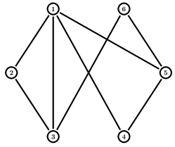
Figure 1: The communication topology.

The objective is to design a distributed controller (3) such that the closed-loop network is quadratically stable for all $\Delta k_{i}$. Let $k_{0}=7N/m$ and $m=2.5kg$. Solving the LMI (10) with $\delta=10$ by using the Sedumi toolbox [36] gives a feasible solution:

$$P=\begin{bmatrix}1.6448&-2.3499\\ -2.3499&9.7007\end{bmatrix},\quad\tau=64.0444.$$

Thus, the feedback gain matrix is chosen as $K=-\begin{bmatrix}0.1126&0.0788\end{bmatrix}$. Assume that the communication topology is given in Fig. 1, with only the first node knowing its own state. In (3), let $d_{1}=2$, and $d_{i}=0$, $i=2,\cdots,6$. Then, the minimal eigenvalue of the matrix $\widehat{\mathcal{L}}$ in (4) is 0.237. Therefore, by Algorithm 1, the controller (3) with $K$ chosen above solves the distributed quadratic stabilization problem for all $\Delta k_{i}$ satisfying $|\Delta k_{i}|\leq 10$, if the coupling strength $c\geq 270.2295$. The simulation result is depicted in Fig. 2, with $c=275$ and $\Delta k_{i}$ randomly chosen within the interval $(7,22]$.

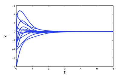
Figure 2: The state trajectories of the agents (38) under controller (3).

By solving the optimization problem (14), it is obtained that the maximal allowable $\delta$ tends to be infinity. It is worth noting that a very large $\delta$ generally implies a high-gain controller (3). For instance, the product of the feedback gain matrix $K$ and the threshold $c_{th}$ corresponding to $\delta=1.5\times 10^{5}$ is obtained as $c_{th}K=-\begin{bmatrix}1.2558&0.0074\end{bmatrix}\times 10^{5}$.

Example 2. The dynamics of the discrete-time agents are given by (24), with

$$A=\begin{bmatrix}1&2&0\\ 0&1&0\\ -1&0&-0.6\end{bmatrix},B=\begin{bmatrix}0\\ 1\\ 1\end{bmatrix},D=\begin{bmatrix}0.8\\ 0\\ 0\end{bmatrix},E=\begin{bmatrix}0&1&0\end{bmatrix}.$$

The communication topology is given as in Fig. 1, with the first and last nodes knowing their own states. In (25), let $\hat{d}_{1}=0.3$, $\hat{d}_{6}=0.5$, and $\hat{d}_{i}=0$, $i=2,\cdots,5$. Thus, the matrix $\widetilde{\mathcal{D}}$ in (26) is

$$\widetilde{\mathcal{D}}=\begin{bmatrix}0.1&0.15&0.15&0.15&0.15&0\\ 0.15&0.5&0.35&0&0&0\\ 0.15&0.35&0.3&0&0&0.2\\ 0.15&0&0&0.1&0.15&0\\ 0.15&0&0&0.15&0.5&0.2\\ 0&0&0.2&0&0.2&0.1\end{bmatrix},$$

whose eigenvalues are -0.1611, -0.0644, 0.0959, 0.2257, 0.6316, 0.8722. Using the Sedumi toolbox [36] to maximize $\delta$ in the LMI (27) with $\kappa=0.9$ yields the largest allowable certainty bound $\delta_{\max}=2.5$ and the corresponding solution are as follows:

$$P =\begin{bmatrix}98.2213&-2.0000&-61.3883\\ -2.0000&0.1197&1.3573\\ -61.3883&1.3573&86.2810\end{bmatrix},$$

$$W =\begin{bmatrix}0&-0.0780&-0.0612\end{bmatrix},\quad\tau=0.0912.$$

Thus, the feedback gain matrix of (25) is obtained as $K=\begin{bmatrix}-0.0195&-0.9888&0.0009\end{bmatrix}$. The state trajectories of network (26) are depicted in Fig. 3, with the uncertainties $F_{i}$ randomly chosen within $[-2.5,2.5]$.

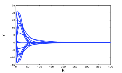
Figure 3: The state trajectories of (26) under controller (25).

6 Conclusion

In this paper, the distributed robust control problems of uncertain linear multi-agent systems have been considered, where the agents are assumed to have identical nominal dynamics while subject to different norm-bounded parameter uncertainties. Distributed controllers have been designed, based on the relative states of neighboring agents and a subset of absolute states of the agents. It has been shown for both the continuous- and discrete-time cases that the distributed quadratic stabilization problems under such controllers are equivalent to the $H_{\infty}$ control problems of a set of decoupled linear systems having the same dimensions as a single agent. Algorithms have been further presented to construct the distributed controllers. An important yet challenging topic for future research is to extend the results of this paper to solve the consensus and formation control problems of uncertain multi-agent systems.

References

- [1] R. Olfati-Saber, J. Fax, and R. Murray, “Consensus and cooperation in networked multi-agent systems,” Proceedings of the IEEE, vol. 95, no. 1, pp. 215–233, 2007.
- [2] J. Fax and R. Murray, “Information flow and cooperative control of vehicle formations,” IEEE Transactions on Automatic Control, vol. 49, no. 9, pp. 1465–1476, 2004.
- [3] F. Borrelli and T. Keviczky, “Distributed LQR design for identical dynamically decoupled systems,” IEEE Transactions on Automatic Control, vol. 53, no. 8, pp. 1901–1912, 2008.
- [4] P. Massioni and M. Verhaegen, “Distributed control for identical dynamically coupled systems: a decomposition approach,” IEEE Transactions on Automatic Control, vol. 54, no. 1, pp. 124–135, 2009.
- [5] R. Olfati-Saber and R. Murray, “Consensus problems in networks of agents with switching topology and time-delays,” IEEE Transactions on Automatic Control, vol. 49, no. 9, pp. 1520–1533, 2004.
- [6] W. Ren and R. Beard, “Consensus seeking in multiagent systems under dynamically changing interaction topologies,” IEEE Transactions on Automatic Control, vol. 50, no. 5, pp. 655–661, 2005.
- [7] W. Ren, “On consensus algorithms for double-integrator dynamics,” IEEE Transactions on Automatic Control, vol. 53, no. 6, pp. 1503–1509, 2008.
- [8] G. Xie and L. Wang, “Consensus control for a class of networks of dynamic agents,” International Journal of Robust and Nonlinear Control, vol. 17, no. 10, pp. 941–959, 2007.
- [9] W. Ren, K. Moore, and Y. Chen, “High-order and model reference consensus algorithms in cooperative control of multivehicle systems,” ASME Journal of Dynamic Systems, Measurement, and Control, vol. 129, no. 5, pp. 678–688, 2007.
- [10] T. Li, M. Fu, L. Xie, and J. Zhang, “Distributed consensus with limited communication data rate,” IEEE Transactions on Automatic Control, vol. 56, no. 2, pp. 279–292, 2011.
- [11] R. Carli, F. Bullo, and S. Zampieri, “Quantized average consensus via dynamic coding/decoding schemes,” International Journal of Robust and Nonlinear Control, vol. 20, no. 2, pp. 156–175, 2009.
- [12] S. Tuna, “Conditions for synchronizability in arrays of coupled linear systems,” IEEE Transactions on Automatic Control, vol. 54, no. 10, pp. 2416–2420, 2009.
- [13] L. Scardovi and R. Sepulchre, “Synchronization in networks of identical linear systems,” Automatica, vol. 45, no. 11, pp. 2557–2562, 2009.
- [14] Z. Li, Z. Duan, G. Chen, and L. Huang, “Consensus of multiagent systems and synchronization of complex networks: A unified viewpoint,” IEEE Transactions on Circuits and Systems I: Regular Papers, vol. 57, no. 1, pp. 213–224, 2010.
- [15] C. Ma and J. Zhang, “Necessary and sufficient conditions for consensusability of linear multi-sgent systems,” IEEE Transactions on Automatic Control, vol. 55, no. 5, pp. 1263–1268, 2010.
- [16] P. Lin and Y. Jia, “Distributed robust consensus control in directed networks of agents with time-delay,” Systems and Control Letters, vol. 57, no. 8, pp. 643–653, 2008.
- [17] Z. Li, Z. Duan, and G. Chen, “On and performance regions of multi-agent systems,” Automatica, vol. 47, no. 4, pp. 797–803, 2011.
- [18] R. Olfati-Saber, “Flocking for multi-agent dynamic systems: Algorithms and theory,” IEEE Transactions on Automatic Control, vol. 51, no. 3, pp. 401–420, 2006.
- [19] H. Su, X. Wang, and Z. Lin, “Flocking of multi-agents with a virtual leader,” IEEE Transactions on Automatic Control, vol. 54, no. 2, pp. 293–307, 2009.
- [20] I. Lestas and G. Vinnicombe, “Scalable decentralized robust stability certificates for networks of interconnected heterogeneous dynamical systems,” IEEE Transactions on Automatic Control, vol. 51, no. 10, pp. 1613–1625, 2006.
- [21] I. Lestas and G. Vinnicombe, “Scalable robust stability for nonsymmetric heterogeneous networks,” Automatica, vol. 43, no. 4, pp. 714–723, 2007.
- [22] U. Jönsson and C. Kao, “A scalable robust stability criterion for systems with heterogeneous LTI components,” IEEE Transactions on Automatic Control, vol. 55, no. 10, pp. 2219–2234, 2010.
- [23] X. Wang, Y. Hong, J. Huang, and Z. Jiang, “A distributed control approach to a robust output regulation problem for multi-agent linear systems,” IEEE Transactions on Automatic Control, vol. 55, no. 12, pp. 2891 –2895, 2010.
- [24] A. Das and F. Lewis, “Distributed adaptive control for synchronization of unknown nonlinear networked systems,” Automatica, vol. 46, no. 12, pp. 2014–2021, 2010.
- [25] W. Ren, “Synchronization of coupled harmonic oscillators with local interaction,” Automatica, vol. 44, no. 12, pp. 3195–3200, 2008.
- [26] Z. Duan and G. Chen, “Global robust stability and synchronization of networks with Lorenz-type nodes,” IEEE Transactions on Circuits and Systems II: Express Briefs, vol. 56, no. 8, pp. 679–683, 2009.
- [27] R. Carli, A. Chiuso, L. Schenato, and S. Zampieri, “Optimal synchronization for networks of noisy double integrators,” IEEE Transactions on Automatic Control, vol. 56, no. 5, pp. 1146–1152, 2011.
- [28] P. Khargonekar, I. Petersen, and K. Zhou, “Robust stabilization of uncertain linear systems: quadratic stabilizability and control theory,” IEEE Transactions on Automatic Control, vol. 35, no. 3, pp. 356–361, 1990.
- [29] L. Xie, M. Fu, and C. de Souza, “ control and quadratic stabilization of systems with parameter uncertainty via output feedback,” IEEE Transactions on Automatic Control, vol. 37, no. 8, pp. 1253–1256, 1992.
- [30] Y. Hong, J. Hu, and L. Gao, “Tracking control for multi-agent consensus with an active leader and variable topology,” Automatica, vol. 42, no. 7, pp. 1177–1182, 2006.
- [31] K. Zhou and J. Doyle, Essentials of Robust Control. Upper Saddle River, NJ: Prentice Hall, 1998.
- [32] S. Boyd, L. El Ghaoui, E. Feron, and V. Balakrishnan, Linear Matrix Inequalities in System and Control Theory. Philadelphia, PA: SIAM, 1994.
- [33] T. Iwasaki and R. Skelton, “All controllers for the general control problem: LMI existence conditions and state space formulas,” Automatica, vol. 30, no. 8, pp. 1307–1317, 1994.
- [34] C. de Souza, M. Fu, and L. Xie, “ analysis and synthesis of discrete-time systems with time-varying uncertainty,” IEEE Transactions on Automatic Control, vol. 38, no. 3, pp. 459–462, 1993.
- [35] M. Fu and L. Xie, “The sector bound approach to quantized feedback control,” IEEE Transactions on Automatic Control, vol. 50, no. 11, pp. 1698–1711, 2005.
- [36] J. Sturm, “Using SeDuMi 1.02, a MATLAB toolbox for optimization over symmetric cones,” Optimization Methods and Software, vol. 11, no. 1, pp. 625–653, 1999.