Suzaku view of X-ray Spectral Variability of the Radio Galaxy Centaurus A : Partial Covering Absorber, Reflector, and Possible Jet Component

Abstract

We observed a nearby radio galaxy, the Centaurus A (Cen A), three times with Suzaku in 2009, and measured the wide-band X-ray spectral variability more accurately than the previous measurements. The Cen A was in the active phase in 2009, and the flux became higher by a factor of 1.5–2.0 and the spectrum became harder than that in 2005. The Fe-K line intensity increased by 20–30% from 2005 to 2009. The correlation of the count rate between the XIS 3–8 keV and PIN 15–40 keV band showed a complex behavior with a deviation from a linear relation. The wide-band X-ray continuum in 2–200 keV can be fitted with an absorbed powerlaw model plus a reflection component, or a powerlaw with a partial covering Compton-thick absorption. The difference spectra between high and low flux periods in each observation were reproduced by a powerlaw with a partial covering Compton-thick absorption. Such a Compton-thick partial covering absorber was for the first time observed for the Cen A. The powerlaw photon index of the difference spectra in 2009 is almost the same as that of the time-averaged spectra in 2005, but steeper by $\sim 0.2$ than that of the time-averaged spectra in 2009. This suggests an additional hard powerlaw component with a photon index of $<1.6$ in 2009. This hard component could be a lower part of the inverse-Compton-scattered component from the jet, whose gamma-ray emission has recently been detected with the Fermi/LAT.

1 Introduction

Radio galaxies host an extended emission from relativistic jets and lobes. Jet emission is extremely enhanced by relativistic effects for blazars, whose jet direction is close to the line of sight, and observed in the multi-wavelength band from radio to TeV gamma-rays. Recently, Fermi gamma-ray space telescope has opened a new era for studying jet emissions, by detecting more than 500 gamma-ray blazars (Abdo et al. 2010a). Furthermore, Fermi detected 10 radio galaxies and revealed that radio galaxies are also gamma-ray emitters (Abdo et al. 2010b). Radio galaxies are important to study the jet structure from the mis-aligned jet direction; jet emissions of blazars are dominated by the central region of jets due to the beaming effect while those of radio galaxies are weighted by the jet outer boundary. Possible jet emission from radio galaxies has been reported from infrared to X-ray band (Chiaberge et al. 1999; Hardcastle et al. 2000; Hardcastle et al. 2006), but the spectral property is still uncertain, especially for FR-I radio galaxies, due to the contribution of the accretion disk.

Centaurus A (Cen A) is the nearest radio galaxy, and its gamma-ray emission has been established by Fermi (Abdo et al. 2009a, 2010c) and HESS (Aharonian et al. 2009), and is the second brightest GeV gamma-ray radio galaxy, following NGC 1275 (Abdo et al. 2009b, 2010b). The GeV gamma-ray emission does not come from the kiloparsec-scale jet but likely from the beamed sub-arcsec jet resolved by VLBI (Abdo et al. 2009c; Mueller et al. 2011). In addition, Fermi found that sub-Mpc giant radio lobes of the Cen A are also GeV gamma-ray emitters (Abdo et al. 2010d). Nonthermal soft X-ray emission from the sub-arcsec jet is suggested for the Cen A (Evans et al. 2004). On the other hand, Chandra resolved the X-ray emission from kiloparsec-scale jets (Kraft et al. 2000). Cen A is the brightest AGN in the hard X-ray band (Tueller et al. 2008), and the X-ray spectrum is very similar to that of Seyfert galaxies (Wang et al. 1986, Kinzer et al. 1995, Rothschild et al. 1999). On the other hand, it seems to smoothly connect to the MeV/GeV emission detected with CGRO COMPTEL/EGRET, like blazars (Steinle et al. 1998, Sreekumar et al. 1999). Suzaku observed the Cen A in 2005, and it was reported that Seyfert-like X-ray emission was dominated (Markowitz et al. 2007). Based on the INTEGRAL time-averaged spectra with a long exposure, Beckmann et al. (2011) also indicated that the origin of the hard X-rays is preferred to be a Seyfert-like emission but the nonthermal emission scenario cannot be ruled out. Another question on the Cen A X-ray spectrum is that the reflection continuum was often not required in the spectral fitting (Rothschild et al. 1999; Markowitz et al. 2007; Rothschild et al. 2011; Beckmann et al. 2011), regardless of the existence of a neutral Fe-K fluorescence line. Therefore, interpretation of the Cen A X-ray spectrum still has several open issues.

However, detailed studies of spectral variation in the hard X-ray band have not been reported yet. Time variability of X-ray spectra gives us important opportunities to decompose the spectral components. The Cen A spectrum is strongly absorbed in the soft X-ray band like Seyfert 2 galaxies, and therefore hard X-ray study of time variation is important. In order to measure the spectral variability in detail, we again observed the Cen A with Suzaku, which enables us to measure the short-term time variation in the hard X-ray band with the best accuracy. In this paper, we report the studies of X-ray spectral variability of the Cen A with Suzaku (Mitsuda et al. 2007). Throughout this paper, we assumed the distance to the Cen A as 3.8 Mpc (Rejkuba 2004), and the errors are shown as a 90% confidence level. We refer to the solar photospheric values (Anders & Grevesse 1989) for the solar abundance ratio of the photoelectric absorption, reflection, and plasma model. The cross-section for absorption models is set to that of Baluci${\rm\acute{n}}$ska-Church & McCammon (1992).

2 Observation and Data Reduction

We observed the Cen A three times with Suzaku on July 20–21, August 5–6, and August 14–16 in 2009, as summarized in table 1. In this paper, we also analyzed the Suzaku data obtained in 2005 in the same way for a comparison. Fugure 1 shows the periods of Suzaku observations on the Swift/BAT light curve . The Cen A entered an active phase since 2007 summer. The 2005 data correspond to the low state, while the 2009 data do to the high state. All the observations were performed with XIS 5x5 or 3x3 modes (Koyama et al. 2007) and normal HXD mode (Takahashi et al. 2007, Kokubun et al. 2007), except for the XIS observation in 2005, which was operated in 5x5, 3x3, or 2x2 modes with 1/4 window option in order to avoid the pile-up. The Cen A was observed at the XIS nominal position in 2005, while it was observed at the HXD nominal position in 2009. The XIS count rate was 7–10 counts sec^-1 in 2009, and thus the pile-up did not occur. We also confirmed no pile-up affections by checking that the results of spectral fittings did not change when we excluded the central 2-arcmin region.

We utilized the data processed with the Suzaku version 2.4 pipeline software, and performed the standard data reduction with criteria such as a pointing difference of $<1.5^{\circ}$, a elevation angle of $>5^{\circ}$ from the earth rim, a geomagnetic cut-off rigidity (COR) of $>$6 GV, and the SAA-elapsed time of $>256$ s. Further selection was applied with criteria such as an earth elevation angle of $>20^{\circ}$ for the XIS, COR$>$8 GV and the SAA-elapsed time (T_SAA_HXD) of $>$500 s for the HXD. XIS photon events were accumulated within 4 arcmin of the Cen A nucleus, with the XIS- 0, 2, and 3 data coadded. The XIS rmf and arf files were created with xisrmfgen and xisarfgen (Ishisaki et al. 2007), respectively, and the XIS detector background was estimated with xisnxbgen (Tawa et al. 2008). For the HXD, the ”tuned” PIN and GSO background was used (Fukazawa et al. 2009) and the good time interval (GTI) was determined by taking the logical-and of GTIs among the data and background model. Since the XIS light-leakage estimation was not valid at the beginning of the 2005 observation, we eliminated the data in the first 12 hours. Note that Markowitz et al. (2007) included this period in the analysis and therefore our results are somewhat different from theirs for absorption model parameters and so on. For the XIS and HXD-PIN, CXB was added to the background spectrum thus obtained, although it is negligible for the HXD-GSO. The latest GSO response file (version 20100524) and the GSO response correction file (version 20100526) were utilized. The former is updated in terms of energy-channel linearity and GSO gain history (Yamada et al. 2011), and the latter compensated for any disagreement of 10–20% between the Crab spectral model and the data .

As a result, a net exposure time for the XIS is around 33 ks, 62 ks, 51 ks, and 56 ks for the 2005, 2009-1st, 2nd, and 3rd observation, respectively. The exposure time for the HXD is about 70% of the XIS ones, due to additional cuts of high background periods. The HXD-PIN signal rate is higher than the background rate below 50 keV, while the HXD-GSO signal rate is $<10$% of the background rate. Therefore, we checked the reproducibility of the GSO background as described in appendix. As a result, the reproducibility of the GSO background is found to be as good as around 1%. Note that the data of the 2009 1st observation was already used in Abdo et al. (2010c).

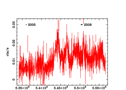
Figure 1: Swift/BAT light curve of the Cen A in the 15–50 keV band . Triangles represent the period of Suzaku observations.

3 Data Analysis

3.1 Light Curves and Correlations

Figure 2 shows the count-rate light curves of the XIS (3–8 keV), PIN (15–40 keV), and GSO (50–100 keV), with a time bin of 10 ks. The background was subtracted for the PIN and GSO, while the XIS background rate is $<1$% of the signal, and thus is negligible. Note that the background rate of the PIN and GSO is around 0.3 and 8–10 count s^-1, respectively. All the observations clearly exhibit time variability in the XIS and PIN light curves with an amplitude of up to 50% and a time scale of 10–20 ks. This time scale is reasonable for the black hole mass of $(0.5-1)\sim 10^{8}M_{\odot}$ (Silge et al. 2005; Krajnovuie et al. 2007; Neumayer et al. 2007). The largest variability occurred during the 2009-1st observation. Looking at the light curves, there is a different variability pattern between the XIS and PIN. For example, at 0–50000 sec (1–5th bin) in the 2009-1st observation, the rising trend of the count rate is linear for the PIN and concave for the XIS. At 0–70000 (29–35th bin) sec in the 2009-3rd observation, the variability pattern is also different between the XIS and PIN. For the GSO light curve, the error is somewhat large, but a similar trend of variability is clearly seen.

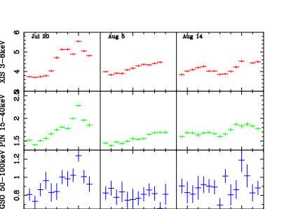
Figure 2: Suzaku light curve of the Cen A for the 2009 Suzaku observations. From top to bottom, XIS-F (3–8 keV), PIN (15–40 keV), and GSO (50–100 keV) are presented. The horizon axis indicates the time bin number with a step of 10000 sec. The beginning of light curves is 55032.328958, 55048.284699, 55057.380162 in MJD, for the 1st, 2nd, and 3rd observation, respectively.

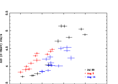
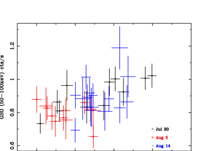
Figure 3: Correlation of count rates of the XIS (3-8keV; left) and the GSO (50-100keV; right) against the PIN (15-40keV). Triangles, circles, and crosses are the data of the 1st, 2nd, and 3rd observation in 2009.

Figure 3 shows a correlation of the count rate among different energy bands. We do not treat the 2005 data, since the XIS to PIN effective area ratio is different between 2005 and 2009 and the data duration of the 2005 observation was short. The XIS count rate in 3–8 keV generally correlates with the PIN count rate in 15–40 keV, but the slope is different among observations. Furthermore, the correlation is not completely linear, especially for the 2009-1st and 3rd observation; the deviation is up to 20% or so. These trends indicate that the spectral shape varied significantly, suggesting multiple spectral components or a change of the spectral shape. On the other hand, considering that the GSO background reproducibility is around 0.1–0.2 count s^-1 (Fukazawa et al. 2009), it can be said that the GSO count rate in 50–100 keV correlates with the PIN count rate within 10–20%. This situation is also the same as that in 100–200 keV. Therefore, the emission in 15–200 keV could be mainly explained by a combination of a variable component and a constant one within errors.

3.2 Modeling of the Soft X-ray Component

The X-ray spectrum of the Cen A is known to consist of roughly two components; a spatially extended component in the soft band and a strongly absorbed hard nuclear component (Markowitz et al. 2007). The former extended component was clearly resolved into many complex features associated with the Cen A jets, such as kiloparsec-jets, shock regions, together with interstellar hot medium and discrete sources in the parent galaxy (Kraft et al. 2008). Especially, shock regions show a relatively hard powerlaw emission (Croston et al. 2009), whose flux is lower by two orders of magnitudes than that of the nuclear X-ray emission. Since the spectral component in the soft band somewhat affects the modeling of the nuclear component, we first modeled the soft component by using the XIS data of the 2009 2nd observation. Before this analysis, we fitted the XIS spectra in 2–10 keV, to model the hard X-ray continuum with the absorbed powerlaw model. Then, we included the model of the hard component whose parameters are fixed to the values obtained above, except for the powerlaw normalization, and fitted the XIS spectra in 0.7–3 keV with one apec thermal plasma model, together with the absorbed powerlaw model. The metal abundance is left free, and the photoelectric absorption model phabs is multiplied. The relative normalization between the XIS-F and XIS-B is let to be free, due to calibration uncertainties associated with attitude fluctuations. We ignored the 1.82–1.84 keV band due to the XIS calibration problems. However, this modeling could not reproduce the spectra with a reduced $\chi^{2}$ values of 4.14, since the apec model cannot simultaneously explain the emission lines and the continuum around 1.5–2 keV where the spectral slope is around 2. Next, we added the bremss model with the absorption to model the extended hard emission from unresolved point sources and jet features in the Cen A (Matsushita et al. 1994). Many sources in the Cen A could contribute to the X-ray emission, but the obtained X-ray luminosity of the bremss component is $8\times 10^{39}$ erg s^-1 (2–10 keV), which can be explained by the sum of X-ray point sources in the Cen A (Kraft et al. 2001) . This is not the matter of this paper, and we do not further discuss about it in this paper. This model made the fit improve, and a reduced $\chi^{2}$ value became 1.44, but the emission lines could not be well reproduced. Markowitz et al. (2007) reported that two-temperature plasma components were required.

We thus added one more apec model whose temperature and abundance are left free. Then, the spectrum is well fitted with the best-fit absorption column density and metal abundance of $1.6\times 10^{21}$ cm^-2 and $\sim 0.3$ solar, respectively, but their errors became larger. The former best-fit value is somewhat larger than that of the Galactic value $8.6\times 10^{20}$ cm^-2 (Dickey & Lockman 1990), implying an additional intrinsic absorber such as interstellar medium within the parent galaxy . We hereafter fixed the absorption column density and metal abundance to the above values. Evans et al. (2004) and Markowitz et al. (2007) reported the detection of Si and S fluorescence lines. In this analysis, the Si-K line is not significant with an upper limit of $7\times 10^{-6}$ c s^-1 cm^-2. Therefore, we include the S-K line at 2.306 keV in the model and then the fit improved with $\Delta\chi^{2}=10$, and its intensity is $1.57_{-0.97}^{+0.70}\times 10^{-5}$ c s^-1 cm^-2. As a result, the soft X-ray spectra could be fitted well with a reduced $\chi^{2}$ values of 1.25, as shown in figure 4 and the best-fit parameters are summarized in table 2.

We also analyzed the XIS spectra of other observations in the same way as above, and the results are summarized in table 2. Since the thermal components are believed to be extended, their parameters should be constant and the best-fit values are consistent among all the observations within errors. In the following broad-band fitting for all the observations, we fixed the temperatures and column densities of the above model to the values in table 2.

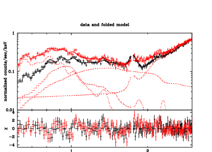
Figure 4: Spectral fitting of the XIS spectra in 2009 2nd observation with the two-temperature apec plasma models plus bremmstrahlung, together with the emission model of the nuclear emission seen above 2 keV. Details are described in the text. Solid line represents the best-fit total emission model, and dotted lines represent each of spectral component; two apec, bremss, and absorbed powerlaw. Red and black ones correspond to the XIS-B and XIS-F, respectively.

Figure 5: Spectral fitting of the XIS/PIN/GSO spectra in 2009 2nd observation with the model A, B, and C. Detailed description of the models are described in the text. Top panel shows the XIS/PIN/GSO spectra with the best-fit model C. 2nd, 3rd, and 4th panels show the residual of the fitting for the model A, B, and C, respectively.

3.3 Time-Averaged Spectrum of Each Observation

Although the spectral variability during each observation is indicated in the previous subsection, we here analyze the time-averaged spectrum of each observation in order to understand the spectral shape. At first, we describe the spectral fitting of the 2009-2nd observation, whose time variability was relatively moderate. After determining the best-fit modeling, we apply it to other observations.

We then fit the XIS-F, XIS-B, PIN, and GSO spectra of the 2009-2nd observation in 0.7–300 keV simultaneously to model the nuclear hard component. For each detector, the energy range of 0.7–10 keV, 15–70 keV, and 55–300 keV for the XIS, PIN, and GSO, respectively, are used in the fitting. A relative normalization between the XIS-F and XIS-B is left to be free, while that between the XIS and PIN, or between the PIN and GSO, is fixed to 1.18 (Maeda et al. 2008) or 1.0 , respectively. The spectral models for the soft X-ray emission were included, but the model parameters of two apec models and bremss model are fixed, and normalizations of the higher-temperature apec model and the bremss model are left free.

For the hard nuclear component, we at first tried the basic model; an absorbed power-law with a Fe-K line (model A). For the strong photoelectric absorption for the nuclear emission, we use the zvphabs model, where the Fe abundance is left free and other elemental abundances are fixed to 1 solar. We tentatively included the high energy cut-off fixed at 1000 keV for the powerlaw model. The broad-band X-ray spectra in 0.7–300 keV are overall fitted with this basic model. The residual of fitting with this model is shown in the 1st panel of figure 5, where a reduced $\chi^{2}$ value is 1.21. However, significant residual structures are seen around 15–30 keV and 50–300 keV. The residual around 15–30 keV could be due to the reflection component, and then we include the pexrav model (Zdziarsk et al. 1995) for the reflection (model B), where the input powerlaw parameters of the pexrav model are tied to those of the direct nuclear powerlaw model and the inclination angle is assumed to be $cos\theta=0.5$ ($\theta=60^{\circ}$); only the free parameter is the reflection fraction $R$. Furthermore, we multiplied the reflection component by the absorption. As shown in the 2nd panel of figure 5, the residual around 15–40 keV still remains a little, but the fit improved with $\Delta\chi^{2}=35$ for addition of two parameters. The reflection fraction became $R=0.19$, while the absorption for the reflection component is not required.

Alternatively, the residual structure in the 1st panel of figure 5 could be reproduced by a partial covering absorption with a column density of $\sim 10^{24}$ cm^-2. Then, instead of the reflection, we included the pcfabs model for representing the partial covering absorption (model C). The fit gave a similar $\chi^{2}$ value (the difference of $\chi^{2}$ is 13) to that for the model B (the 3rd and 4th panels in figure 5). The best-fit model gave an column density of $(2.7\pm 1.1)\times 10^{23}$ cm^-2 and a covering fraction of 9$\pm$3% for the partial covering absorber.

We applied the above models to other observations. Since the observational detector position of the Cen A is different between 2005 and 2009, a relative normalization between the XIS and PIN is different. Unlike 2009, the position of the 2005 observation is not nominal and thus a nominal relative ratio of normalizations is not available. Therefore, we at first set a relative normalization between the XIS and PIN to be free, and obtained it to be 1.06. This is consistent with the value in Markowitz et al. (2007). Accordingly, we hereafter fixed the relative normalization to 1.06 for the 2005 observation.

The fitting results of four observations for the model A, B, and C are summarized in table 3–5. The model B and C gave a better fit than the model A for all the observations, and they gave a similar $\chi^{2}$ value for 2009 three observations, while the model C gave a significant improvement of the fitting for the 2005 observation. Markowitz et al. (2007) reported a similar trend for the 2005 observation. Figure 6 compares the $\nu F\nu$ spectra of all observations, and Figure 7 shows the best-fit $\nu F\nu$ spectra of the 2009 2nd observation. It can be seen that the soft X-ray emission in 0.7–2 keV is at almost the same flux level because the emission comes from the extended region, while the hard X-ray emission brightened in 2009; 0.2 keV cm^-2 s^-1 and 0.2 keV cm^-2 s^-1 at 20 keV and 100 keV, respectively, in 2005, 0.3–0.4 keV cm^-2 s^-1 and 0.4–0.5 keV cm^-2 s^-1 at 20 keV and 100 keV, respectively, in 2009. In the following, let us look at the fitting results for the model C. The column density of uniform absorber is almost constant at $1.0\times 10^{23}$ cm^-2 for all the observations. The covering fraction of the partial covering absorber is around 30% in 2005, while it is around 8–10% in 2009. The column density of the partial covering absorber is not constant, but two observations in 2009 gave a Compton-thick value of $>10^{24}$ cm^-2. The large difference appears for the powerlaw photon index; 1.94 in 2005 and 1.68–1.71 in 2009. In other words, the Cen A spectrum became significantly harder in 2009 as can be seen in figure 7. The intensity of the neutral Fe-K fluorescence line is $(2.3\pm 0.2)\times 10^{-4}$ c s^-1 cm^-2 in 2005 and $(2.7-2.9)\times 10^{-4}$ c s^-1 cm^-2 in 2009. This is the first evidence of variability of the Fe-K line intensity for the Cen A, and the Fe-K line intensity is considered to be high in 2009 as a result of brightening of the Cen A continuum emission since 2007.

Although the time-averaged spectra can be fitted with the model B or C, both of the models have a problem. For the model B, the reflection component is generally considered to be constant and thus only the powerlaw component cannot explain the complex time variability as described in §3.1. The fluorescence Fe-K line is significantly detected with an equivalent width (EW) of 78, 56, 69, 56 eV for the 2005, 2009 1st, 2009 2nd, 2009 3rd observation, respectively, indicating that there is an underlying reflection continuum and thus the model C does not match this evidence. The reflection fraction in the model B is around 0.19–0.34 in 2009 and 0.41 in 2005. The EW of the Fe-K line against the reflection component is 1.0–2.0 keV, and this is reasonable for the Compton-thick reflector with one solar abundance. Therefore, both of the reflection component and the partial covering absorption are likely to be required.

The above results are obtained by assuming that the exponential cut-off energy of the powerlaw model is 1000 keV. Then, we let it free for the model C, but only a lower limit of $\sim 500$ keV is obtained both in 2005 and 2009. Therefore, hereafter, we fixed the cut-off energy to 1000 keV.

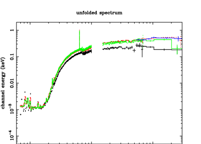
Figure 6: $\nu F\nu$ plots of the XIS/PIN/GSO spectra for all observations. Black, red, green, blue data correspond to the spectrum of the 2005, 2009 1st, 2009 2nd, 2009 3rd observation, respectively.

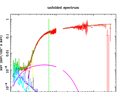
Figure 7: $\nu F\nu$ plots of the XIS/PIN/GSO spectra with the model C for the 2009 2nd observation.

3.4 Difference Spectra between High and Low Flux Periods

Before performing the spectral fitting by including both of the reflection and the partial covering absorption, it is important to study the spectral component which produces the complex time variability. Here, we investigated the difference spectra between high and low flux periods in 2009 observations. We used the XIS-F and HXD-PIN data for this analysis, since the XIS-B and HXD-GSO did not give an enough signal-to-noise ratio for this analysis.

First, we took a difference spectrum between high and low flux periods in each observation. We defined high and low flux periods in figure 2 as follows: 8–11th bin, 22–24th bin, and 39–42th bin for high flux periods, and 1–4th bin, 15–17th bin, and 29–32th for low flux periods. We fitted the difference spectra defined as above with an absorbed powerlaw model, which typically represents the difference spectra of Seyfert galaxies (e.g. Miniutti et al. 2007; Shirai et al. 2008). Figure 8 shows the fitting results for the 1st observation. Overall spectral shape is represented by the absorbed powerlaw model, but the fit is not good with a reduced $\chi^{2}$ value of 2.33. There is a strong Fe-K edge feature in the observed spectrum and it is not reproduced well by the best-fit model. This indicated a thicker absorber, and thus we tried a partial covering absorption model. Then, the fit improved with $\Delta\chi^{2}=36$, and the edge feature can be fitted with this model. Figure 9 shows a confidence contour between the partial covering fraction and photon index. The Compton-thick absorber of $N_{\rm H}=2.6\times 10^{24}$ cm^-2 with a high covering fraction of 0.64 is required by the deep Fe-K edge structure. The powerlaw photon index is 2.23$\pm$0.18, somewhat steeper than that for the time-averaged spectra.

For other two observations, since the signal-to-noise ratio of spectra is not high, the Fe-K edge-feature is less clearer. However, when the spectra are fitted by a powerlaw model with a simple absorption, the photon index becomes very small; $1.4\pm 0.2$ and $1.2\pm 0.2$ for the 2nd and 3rd observation, respectively. When the partial covering absorption model is introduced, the powerlaw photon index becomes reasonable around 2 for the 2nd observation. This is not the case for the 3rd observation; errors of photon index and absorption column density are large. When we fixed the photon index to 2.0 for the 3rd observation, the absorption column density of the uniform absorber becomes reasonable around $1\times 10^{23}$ cm^-2. The fitting results are summarized in table 6. The partial absorber has a large column density of $>10^{24}$ cm^-2 with a large covering fraction of $>0.3$, and they seem variable. These behaviors could cause a complex time variability. Such a Compton-thick absorber was for the first time observed for the Cen A.

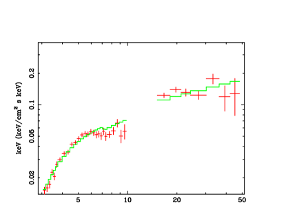
Figure 8: $\nu F\nu$ plot of the difference spectra of the XIS/PIN between high and low periods in the 2009 1st observation. The solid line represents a powerlaw model with a simple absorption.

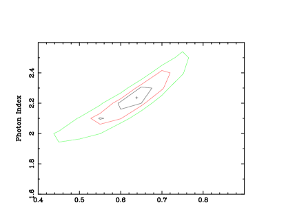
Figure 9: Confidence contour between the partial covering fraction of absorption and powerlaw photon index.

The partial covering absorber is thought to be variable during each observation. Therefore, next, we investigated a spectral variability with a finer time resolution. We divided one observation into several periods with a step of 10 ks, following the light curve in figure 2, and took a difference spectrum between two periods, one of which is the low flux period just before brightening and the other is around the highest flux level. We took the difference between 7th and 3rd bin during the 1st observation, 10th and 9th during the 1st observation, 24th and 16th bin during the 2nd observation, 41th and 38th bin during the 3rd observation in figure 2. Table 6 summarized the fitting results of the partial covering absorption model with the photon index fixed to 2.0. Since the signal-to-noise ratio of each spectrum is not so high, errors are large. However, the column density and covering fraction are not constant while the column density of the uniform absorber is constant around $1\times 10^{23}$ cm^-2.

In summary, the complex time variability of the Cen A is likely to be caused by the variability of the partial covering absorber with a time scale of $<10000$ sec, while the powerlaw photon index is almost stable around 2.0.

3.5 Additional Hard Powerlaw Component

Since the partial covering absorber is found to exist by the study of spectral variability, both of the reflection and the partial covering absorber are needed to fit the Suzaku wide-band X-ray spectra of the Cen A. Then, we fitted the time-averaged spectrum of each observation by considering both of spectral features (model D). The fitting results are summarized in table 7. The reduced $\chi^{2}$ is almost the same as that of the model C (partial covering absorption without reflection), and the reflection continuum is not required. This is inconsistent with the existence of the Fe-K line. Another problem is that the powerlaw photon index of 1.7 for the time-averaged spectra in 2009 is different from that obtained by the analysis of the difference spectra, which require the photon index of $\sim$2.

The powerlaw component is generally thought to be due to thermal Comptonization of disk photons, as well as the low/hard state of black hole binaries. For Cyg X-1 and GX 339-4, when they are brighter in the low/hard state, the Compton thickness becomes larger but the Comptonizing electron temperature becomes lower (Makishima et al. 2008, Zdziarski et al. 2004, Del Santo 2008). As a result, the powerlaw photon index and cut-off energy are larger and lower, respectively; in other words, the spectrum becomes softer in the brighter phase. A bright Seyfert galaxy, NGC 4151, also exhibited such a trend (Lubi${\rm\acute{n}}$ski et al. 2010). On the other hand, the trend of the Cen A is opposite; the spectrum became harder in the bright phase.

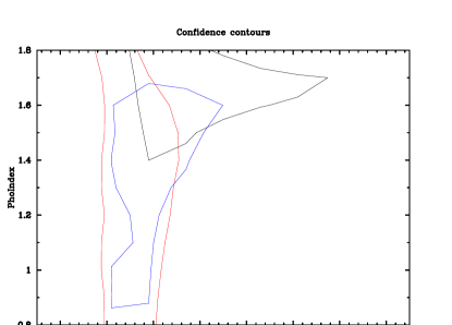
Figure 10: Confidence contour between the soft and hard powerlaw photon index for fitting with the model E. The contours represent a 95% confidence level for each observation. Black solid, red dashed, and blue dotted lines correspond to those of 2009 1st, 2nd, and 3rd observation, respectively.

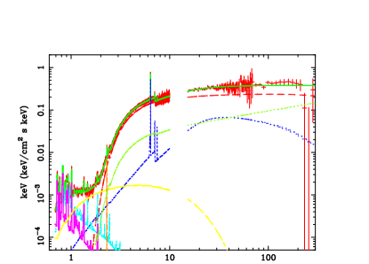
Figure 11: $\nu F\nu$ plot of the XIS/PIN/GSO spectra of the 2009 2nd observation with the model E.

The Cen A has been found to be a gamma-ray emitter up to the TeV band, while black hole binaries and NGC 4151 are not. Therefore, the nonthermal jet component, which connects to the high energy gamma-ray band, is expected to exist in the X-ray band. We included one more powerlaw model in addition to the model D, and multiplied it by the absorption with a column density of $1\times 10^{23}$ cm^-2; the absorption is needed for this additional powerlaw component to be below the observed flux in the soft X-ray band, and the above value is just assumption. Later we describe about the dependence of results on this absorption. In this case, we cannot constrain the parameters of both powerlaw components well. In addition, the intensity of the hard powerlaw component becomes coupled with that of the reflection component. Then, we replaced the pexrav model by the pexmon model (Nandra et al. 2007) for the reflection component. The pexmon model considered the Fe-K and Ni-K fluorescence lines and thus we can constrain the reflection component by the prominent Fe-K line. In this case, the gaussian model for the Fe-K line is not included for fitting (model E).

Figure 10 shows a confidence contour between the soft and hard powerlaw photon index, where we plot the 95% confidence contours of three 2009 observations. The photon index of the soft and hard component is constrained to be around 1.9 and 1.6, respectively, for all 2009 observations. The photon index of the hard component depends on the assumed absorption; when the absorption is weaker, the photon index becomes smaller and the fraction of the hard component in the softer X-ray band becomes smaller. Thus the photon index of 1.6 is considered to give an upper limit of the hard component. Then, we fixed the photon indices of the two powerlaw components to 1.6 and 1.9. Table 8 summarized the fitting results, and figure 11 shows the best-fit model and spectra. The $\chi^{2}$ value is smaller than those of the model D for the 2009 1st observation, but almost the same as those of the model D for others. The fraction of the reflection component is around 0.4–0.5 and the Fe abundance is around 0.7–0.9 solar, These are typical values for Seyfert galaxies, and therefore reasonable values; it can be said that we correctly model the reflection component. The flux of the additional powerlaw component was $<$10% and 30% of the original powerlaw at 100 keV in 2005 and 2009, respectively. Therefore, the flux increase of the additional hard powerlaw component, possibly associated with the jet, can explain the harder spectra in 2009, but the Seyfert-like component is still dominant in the Suzaku X-ray band even if the jet component exists.

3.6 Time History of Spectral Parameters

In order to check the view of the model E, we performed time-resolved spectral fittings for the 2009 observations. We divided the XIS, PIN, and GSO data of each observation into 11–14 periods as a step of 10 ks. Each period corresponds to each bin of the light curve in figure 2. Since the signal-to-noise ratio is low, we fixed the following parameters to the best-fit values obtained for the time-averaged spectra of each observation in table 8; reflection fraction, normalization of reflected powerlaw emission, Fe abundance of absorber and reflector, normalization of the S-K line, parameters of the soft thermal components. Then, free parameters are a column density of the uniform absorber, a column density and covering fraction of the thicker absorber, and normalizations of two powerlaw component. In addition, we ignored the data below 3 keV, where the thermal component is dominant.

Figure 12 shows a time history of spectral parameters. The column density of the uniform absorber is less variable; with at most 10% variability. The most variable parameters are the normalization of the lower energy powerlaw component, the column density and covering fraction of the thicker absorber. This could create a complex correlation behavior in subsection 3.1. The normalization of the higher energy powerlaw component is almost constant, but a small variability is seen for the 3rd observation. It shows an anticorrelation with the normalization of the lower energy powerlaw component, and therefore this could be artificial. No clear correlation between the lower and higher energy powerlaw components suggests a different origin between two components.

Figure 12: Time history of the spectral parameters of the model E for the 10ks-time-resolved spectra in 2009 observations. The horizontal number corresponds to the time bin number in figure 2. From top to bottom, an uniform absorption column density in unit of $10^{22}$ cm^-2, a partial covering absorption column density in unit of $10^{22}$ cm^-2, a partial covering fraction of absorption, and normalizations of the soft and hard powerlaw component in unit of ph cm^-2 s^-2 keV^-1 at 1 keV, are shown.

4 Discussion

In summary, we measured the broad-band X-ray spectral variability of the Cen A more accurately than ever with Suzaku, and found that the variable component is a powerlaw with a partially covering Compton-thick absorption of $\sim 10^{24}$ cm^-2. We also found a variability of the Fe-K line intensity from 2005 to 2009 by a factor of 1.3 or so. The reflection component associated with the Fe-K line is also suggested in the spectral modeling, and furthermore an additional hard powerlaw component with a photon index of $<1.6$ is inferred.

4.1 Origin of X-ray Time Variability

X-ray time variability of the Cen A has been reported with the CGRO/BATSE, CGRO/OSSE, RXTE, XMM-Newton, INTEGRAL, and Swift/BAT, for various time scales from sub-days to years (Kinzer et al. 1995, Wheaton et al. 1996, Rothschild et al. 1999, Rothschild et al. 2006, Evans et al. 2004).

RXTE and INTEGRAL observations reported that the time variability is caused by the change of absorption column density, the powerlaw photon index, and the powerlaw normalization, based on the spectral fitting by a powerlaw model with an uniform absorption (Rothschild et al. 2006). The absorption column density is in the range of $(0.9-1.7)\times 10^{23}$ cm^-2, the powerlaw photon index is in the range of 1.65–1.85, and the flux is $(4-10)\times 10^{-10}$ erg cm^-2 in 20–100 keV. For the Suzaku observations (table 3), the column density is $(0.9-1.2)\times 10^{23}$ cm^-2, the powerlaw photon index is in the range of 1.65–1.82, and the powerlaw flux in 20–100 keV is $5.7\times 10^{-10}$ erg cm^-2 s^-1 and $11\times 10^{-10}$ erg cm^-2 s^-1 in 2005 and 2009, respectively, based on the same model. Therefore, the spectral parameters match the past observations. However, the accurate spectroscopy with Suzaku revealed that a powerlaw model with an uniform absorption was not valid, and the X-ray variation is partly caused by the change of the partial covering Compton-thick absorber, together with the change of the powerlaw continuum level with a time scale of sub-days. The absorption column density of the uniform one is almost constant around $1.2\times 10^{23}$ cm^-2.

The variability of the Fe-K line has never been reported in the past observations; it is steady around $5\times 10^{-4}$ ph cm^-2 s^-1. Suzaku for the first time confirmed that the Fe-K line intensity significantly increased by a factor of several tens percents from 2005 to 2009, following the brightening of the continuum flux since 2007. This suggests that the Fe-K line emitter lies at a distance of $<1$ pc from the nucleus. The Fe-K line intensity observed with Suzaku is $(2.3-3.0)\times 10^{-4}$ ph cm^-2 s^-1, and therefore it is relatively weaker than ever. RXTE results reported that the Fe-K line intensity is around $5\times 10^{-4}$ ph cm^-2 s^-1 in 2004, just before the Suzaku 2005 observation. However, we must take care that the RXTE energy resolution of $\sim$1000 eV cannot accurately resolve a Fe-K line with an EW of $\sim$100 eV. Chandra and XMM-Newton results of $(2-4)\times 10^{-4}$ ph cm^-2 s^-1 (Evans et al. 2004) were close to the Suzaku ones.

The behavior in the soft gamma-ray band was well studied with the OSSE (Kinzer et al. 1995); the spectral cut-off shape varied in such a way that the cut-off was clearer in the bright phase (0.6 keV cm^-2 s^-1 at 100 keV) than in the faint phase (0.2 keV cm^-2 s^-1 at 100 keV). Suzaku 2005 data correspond to the faint phase, and the 2009 data do to the bright phase. However, the spectral cut-off is not clearly detected with Suzaku both in 2005 and 2009. This would be related with the additional powerlaw component, and we discuss this issue in the following subsection.

4.2 X-ray Reprocessing Materials

The location of the stable uniform absorber can be constrained by the Fe-K edge which is almost attributed to the uniform absorber for the time-averaged spectra. The edge energy is $7.12\pm 0.03$ keV in 2009, leading to the ionization parameter of $\xi=\frac{L}{nR^{2}}\leq 0.1$, where $L$ is the luminosity of the central engine, $n$ the matter density, and $R$ the distance to the matter (Kallman et al. 2004). Considering the column density $N_{\rm H}<nR$, the uniform absorber lies at $>160$ pc away from the nucleus, where we take $L=5\times 10^{42}$ erg s^-1 and $N_{\rm H}=1\times 10^{23}$ cm^-2. Therefore, the uniform absorber is likely to be associated with the famous dust lane lying on the elliptical galaxy.

On the other hand, the location of the thicker partial covering absorber can be constrained by the Fe-K edge in the difference spectra between high and low flux states; the edge energy is $<7.3$ keV, corresponding to $\xi\leq 10$. In the same way as above, using $N_{\rm H}=10^{24}$ cm^-2, the location is constrained to be $R>0.16$ pc. The variation of absorber parameters with a time scale of $\delta t\sim 1$ day indicates the blob-like structure. Taking the black hole mass of $5\times 10^{7}$ $M_{\odot}$, the Kepler velocity is $v=1.1\times 10^{8}$ cm s^-1 at a radius of 0.16 pc. Then, the size of blobs perpendicular to the line of sight becomes $v\delta t\sim 10^{13}$ cm. Since the size toward the line of sight is likely to be the same order as above, the density becomes $n\sim 10^{11}$ cm^-3.

The Fe-K line EW is typical for Seyfert galaxies with a similar absorption column density (Fukazawa et al. 2011). This indicates that there is a Compton-thick material covering a large solid angle of $\sim\pi$ or so. Considering the variation time scale of $<2$ year, the material is a molecular torus which is believed to exist commonly in Seyfert galaxies. The intrinsic emission irradiating the material is unlikely to be the beamed jet emission, since the jet emission concentrates within a small solid angle along the jet direction by the relativistic effect. Therefore, the Seyfert-like emission originating from the inner disk region is thought to dominate in the X-ray band.

4.3 Jet Component

Our analysis of the Suzaku data suggests the additional hard powerlaw component with a photon index of $<1.6$, whose flux is around 30% of the total flux at 100 keV. This hard component might be brighter in 2009 active phase than in 2005 faint phase. The crossover energy against another powerlaw emission, which is likely to be a Seyfert-like nuclear emission dominated below 100 keV, is around 400 keV. This hard component seems to smoothly connect to the CGRO/COMPTEL MeV gamma-ray emission as shown in figure 13. CGRO/EGRET and Fermi/LAT detected the GeV gamma-ray emission from the Cen A, whose spectrum well connects to the MeV emission. As reported by Abdo et al. (2010c), the multi-wavelength spectrum of the Cen A can be modeled by the Synchrotron Self-Compton model. The predicted jet flux in the X-ray band strongly depends on the model parameters, such as magnetic field, emission size, low energy electron spectrum, and so on (Abdo et al. 2010c). Both of decelerating jet (Georganopoulos & Kazanas 2003) and structure jet (Chiaberge et al. 2000) can explain the X-ray emission inferred in this paper, and the possible hard component obtained by the Suzaku data could be a lower energy part of the Compton component.

Evans et al. (2004) suggested the jet emission in the soft X-ray band with a photon index of around 2 and a flux of $\sim 1\times 10^{-2}$ keV cm^-2 s^-1. This flux is somewhat lower than the hard component suggested with Suzaku, but could be the same component. However, as Evans et al. (2004) described, their soft component can be explained by the leaked nuclear component due to the partial covering absorber. Or, since Evans et al. (2004) did not include the reflection continuum in the spectral model, their soft component could be a reflection continuum which we considered in the spectral fitting. Alternatively, their soft component might be synchrotron emission from jets and the X-ray band covers the transition region from synchrotron emission to inverse Compton scattering. Anyway, we cannot conclude whether their origins are the same or not. .

Jet emission has been detected in the X-ray band for a radio galaxy 3C120 with Suzaku (Kataoka et al. 2007); where the variable soft X-ray component was detected with a shorter time scale than the Seyfert-like nuclear emission. For the Cen A, the possible jet X-ray component has a longer time scale of variability than the Seyfert-like emission. Considering that GeV gamma-ray emission shows no significant variability over one year (Abdo et al. 2010c), the jet emission is less beamed and thus the relativistic effect on the variability is smaller. The jet emission in the X-ray band is often not well understood for other radio galaxies. ASTRO-H/SGD will give us the first opportunity to detect the hard excess component clearly from the Cen A and other radio galaxies. Also, the ASTRO-H can search for the jet emission from the X-ray spectral variability with the sensitive wide-band X-ray spectroscopy, as well as the Cen A and 3C120.

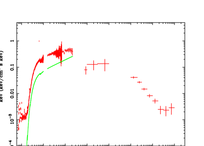
Figure 13: $\nu F\nu$ plot of the Cen A from the X-ray to GeV gamma-ray band. Data points are obtained with the Suzaku (2009), CGRO/COMPTEL (1991–1994), and Fermi/LAT (2008–2009). The solid line represents the hard powerlaw component suggested with the Suzaku observation.

Authors thanks to Dr. J. Kataoka and the anonymous referee for careful reading and helpful comments. The authors also wish to thank all members of the Suzaku Science Working Group, for their contributions to the instrument preparation, spacecraft operation, software development, and in-orbit calibration. This work is partly supported by Grants-in-Aid for Scientific Research by the Ministry of Education, Culture, Sports, Science and Technology of Japan (20340044).

Appendix A GSO background reproducibility for the Cen A data

Since the GSO signal rate from the Cen A is less than 10% of the GSO background, the systematic uncertainty of the GSO background reproducibility is not ignored. Then, we checked the reproducibility by using the earth occultation data during the 2009 Cen A observation. Since the CXB is negligible, we expect no extra signal than the background. Figure 14 shows the comparison of GSO spectra between the earth occultation data and background model, indicating that the background model well reproduce the earth occultation spectra with an accuracy of 2% or so. Figure 15 shows the comparison of GSO light curve between the earth occultation data and background model, indicating that the background model well reproduce the history of the earth occultation rate with an accuracy of 2% or so. Therefore, the background reproducibility is as good as 1%.

For the 2005 observation, no earth occultation occurred during the observation. However, the background rate is lower by a factor of $\sim 2$ than the 2009 observation. Therefore, the effect of the background uncertainty is expected to be smaller.

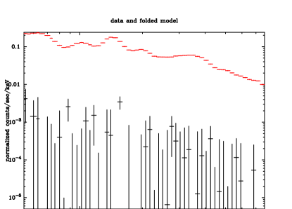
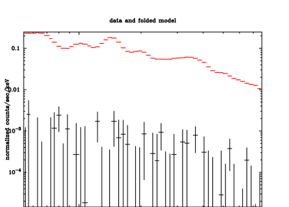
Figure 14: Comparison of GSO spectra between the data and background model during the earth occultation period in each observation.

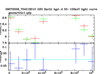
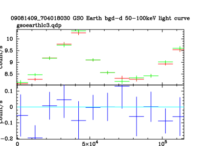
Figure 15: Comparison of GSO light curves in 50–100 keV between the data and background model during the earth occultation period in each observation.

Table 1: Summary of Suzaku observations of the Cen A.

Observation ID	Date	Start	Stop	Exposure⋆
100005010	Aug. 19–20, 2005	08-19 03:39:19	08-20 09:50:08	37984
704018010	Jul. 20–21, 2009	07-20 08:55:29	07-21 18:26:24	44587
704018020	Aug. 5–6, 2009	08-05 07:23:27	08-06 16:52:14	35093
704018030	Aug. 14–16, 2009	08-14 09:06:56	08-16 02:31:24	37636
$\star$: Exposure time of th HXD-PIN data after data reduction.

Table 2: Fitting results of the XIS soft thermal components.

Obs	$I_{\rm bremss}^{a}$	$kT_{1}$	$I_{apec1}^{b}$	$kT_{2}$	$I_{apec2}^{c}$	$\chi^{2}/dof$
	($10^{-3}$)	(keV)	($10^{-3}$)	(keV)	($10^{-3}$)	($\chi^{2},dof$)
2005	1.5$\pm$0.1	0.71$\pm$0.02	1.7$\pm$0.3	0.32$\pm$0.01	3.9$\pm$0.8	2.02 (616.8/306)
2009a	1.6$\pm$0.1	0.72$\pm$0.03	1.8$\pm$0.4	0.33$\pm$0.03	3.8$\pm$1.2	1.49 (455.2/306)
2009b	1.8$\pm$0.1	0.79$\pm$0.05	1.6$\pm$0.5	0.29$\pm$0.01	5.3$\pm$0.5	1.25 (389.9/313)
2009c	1.7$\pm$0.1	0.72$\pm$0.04	2.0$\pm$0.5	0.28$\pm$0.02	4.9$\pm$1.5	1.30 (398.2/306)
Adapted Valuesd	–	0.72	–	0.30	4.0	–
Two apec models are multiplied by the photoelectric absorption, whose absorption column density is fixed to $1.6\times 10^{21}$ cm-2.
Metal abundances of both apec models are fixed to 0.3 solar. A temperature of the bremmstrahlung is fixed to 7 keV.
$a$: Normalization of the bremmstrahlung.
$b$: Normalization of the apec model 1.
$c$: Normalization of the apec model 2.
$d$: Adapted values of spectral parameters for fitting the wide-band Suzaku spectra.

Table 3: Results of simultaneous fitting of the XIS/PIN/GSO spectra (model A^†).

Parameters		2005	2009a	2009b	2009c
$N_{\rm H}^{a}$	($10^{23}$)	1.20$\pm$0.01	0.93$\pm$0.01	1.03$\pm$0.01	1.04$\pm$0.01
$A_{\rm Fe}^{b}$	(solar)	0.65$\pm$0.05	1.53$\pm$0.06	1.10$\pm$0.07	1.09$\pm$0.06
$\alpha_{\rm ph}^{c}$		1.82$\pm$0.05	1.64$\pm$0.05	1.68$\pm$0.06	1.67$\pm$0.05
$I_{\rm pow}^{d}$		0.117$\pm$0.003	0.117$\pm$0.003	0.117$\pm$0.003	0.126$\pm$0.003
$E_{\rm Fe}^{e}$	(keV)	6.398$\pm$0.004	6.392$\pm$0.006	6.394$\pm$0.007	6.395$\pm$0.008
$I_{\rm Fe}^{f}$	($10^{-4}$)	2.6$\pm$0.2	2.6$\pm$0.3	3.0$\pm$0.3	2.7$\pm$0.3
$\chi^{2}/dof$		1.85	1.50	1.14	1.31
($\chi^{2},dof$)		(2314.7/1248)	(2093.4/1392)	(1539.8/1353)	(1796.7/1369)
$\dagger$: Model A is constant*phabs*( [highecut*zvphabs*powerlaw + zgauss] + apec + apec + phabs*bremss + zgauss) in xspec. Components between parentheses [ ] represent the AGN emission.
$a,b$: Hydrogen column density and Fe abundance of the absorber. The column density is in unit of cm-2 for the zvphabs model.
$c,d$: Photon index and normalization at 1 keV of the power-law model.
$e,f$: Center energy and normalization of the Fe-K$\alpha$ line. The normalization is in unit of ph cm-2 s-1.

Table 4: Results of simultaneous fitting of the XIS/PIN/GSO spectra (model B^†).

Parameters		2005	2009a	2009b	2009c
$N_{\rm H}^{a}$	($10^{23}$)	1.25$\pm$0.01	1.01$\pm$0.01	1.07$\pm$0.01	1.08$\pm$0.01
$A_{\rm Fe}^{b}$	(solar)	0.46$\pm$0.03	1.14$\pm$0.05	0.94$\pm$0.06	0.86$\pm$0.07
$\alpha_{\rm ph}^{c}$		1.90$\pm$0.05	1.73$\pm$0.05	1.73$\pm$0.06	1.72$\pm$0.06
$I_{\rm pow}^{d}$		0.127$\pm$0.003	0.132$\pm$0.003	0.126$\pm$0.004	0.131$\pm$0.004
$E_{\rm Fe}^{e}$	(keV)	6.398$\pm$0.004	6.391$\pm$0.006	6.396$\pm$0.006	6.396$\pm$0.007
$I_{\rm Fe}^{f}$	($10^{-4}$)	2.7$\pm$0.2	2.7$\pm$0.3	3.1$\pm$0.3	2.8$\pm$0.3
$R^{g}$	($\Omega/2\pi$)	0.406$\pm$0.002	0.345$\pm$0.003	0.192$\pm$0.004	0.220$\pm$0.005
$\chi^{2}/dof$		1.71	1.42	1.11	1.23
($\chi^{2},dof$)		(2129.7/1246)	(1968.6/1390)	(1505.0/1351)	(1683.6/1367)
$\dagger$: Model B is constant*phabs*( [highecut*zvphabs*powerlaw + zgauss + phabs*pexrav] + apec + apec + phabs*bremss + zgauss) in xspec. Components between parentheses [ ] represent the AGN emission.
$a,b$: Hydrogen column density and Fe abundance of the absorber. The column density is in unit of cm-2 for the zvphabs model.
$c,d$: Photon index and normalization at 1 keV of the power-law model.
$e,f$: Center energy and normalization of the Fe-K$\alpha$ line. The normalization is in unit of ph cm-2 s-1.
$g$: Fraction of the reflection component for the pexrav model.

Table 5: Results of simultaneous fitting of the XIS/PIN/GSO spectra (model C^†).

Parameters		2005	2009a	2009b	2009c
$N_{\rm H}^{a}$	($10^{23}$)	1.17$\pm$0.04	0.97$\pm$0.03	1.01$\pm$0.03	1.05$\pm$0.04
$A_{\rm Fe}^{b}$	(solar)	0.51$\pm$0.10	1.33$\pm$0.11	1.11$\pm$0.08	0.93$\pm$0.11
$\alpha_{\rm ph}^{c}$		1.94$\pm$0.46	1.68$\pm$0.30	1.71$\pm$0.31	1.69$\pm$0.43
$I_{\rm pow}^{d}$		0.176$\pm$0.040	0.138$\pm$0.021	0.129$\pm$0.020	0.138$\pm$0.029
$E_{\rm Fe}^{e}$	(keV)	6.398$\pm$0.005	6.392$\pm$0.006	6.395$\pm$0.007	6.396$\pm$0.007
$I_{\rm Fe}^{f}$	($10^{-4}$)	2.3$\pm$0.2	2.7$\pm$0.3	2.9$\pm$0.3	2.8$\pm$0.3
$N_{\rm H,2}^{g}$	($10^{24}$)	0.41$\pm$0.04	1.58$\pm$0.33	0.27$\pm$0.11	1.10$\pm$0.27
$f_{\rm NH2}^{h}$		0.29$\pm$0.03	0.10$\pm$0.02	0.09$\pm$0.03	0.08$\pm$0.03
$\chi^{2}/dof$		1.43	1.42	1.11	1.23
($\chi^{2},dof$)		(1783.8/1245)	(1970.6/1390)	(1494.2/1351)	(1677.6/1367)
$\dagger$: Model C is constant*phabs*( [pcfabs*highecut*zvphabs*powerlaw + zgauss] + apec + apec + phabs*bremss + zgauss) in xspec. Components between parentheses [ ] represent the AGN emission.
$a,b$: Hydrogen column density and Fe abundance of the absorber. The column density is in unit of cm-2 for the zvphabs model.
$c,d$: Photon index and normalization at 1 keV of the power-law model.
$e,f$: Center energy and normalization of the Fe-K$\alpha$ line. The normalization is in unit of ph cm-2 s-1.
$g,h$: Hydrogen column density and covering raction of the absorber for the pcfabs model.

Table 6: Results of spectral fitting of the XIS/PIN difference spectra with a powerlaw model with a partial covering absorption.

Observation		$N_{\rm H1}^{a}$	$\alpha^{b}$	$N_{\rm H2}^{c}$	$f_{\rm NH2}^{d}$
		$10^{22}$		$10^{24}$
2009 1st	High–Low	$13.2\pm 1.3$	$2.23\pm 0.18$	$2.67\pm 0.98$	$0.64\pm 0.09$
2009 2nd	High–Low	$11.7\pm 6.5$	$2.08\pm 0.81$	$>1.00$	$0.65\pm 0.43$
2009 3rd	High–Low	$11.6\pm 0.7$	2 (fix)	$>0.51$	$0.72\pm 0.17$
2009 1st	7–3th	$13.6\pm 2.1$	2 (fix)	$>0.57$	$0.29\pm 0.21$
2009 1st	10–9th	12(fix)	2 (fix)	$>1.19$	$0.64\pm 0.15$
2009 2nd	24–16th	$11.4\pm 3.0$	2 (fix)	$>1.31$	$0.71\pm 0.13$
2009 3rd	41–38th	12(fix)	2 (fix)	$>0.03$	$0.60\pm 0.25$
$a$: Hydrogen column density of the uniform absorber in unit of cm-2.
$b$: Photon index and normalization at 1 keV of the power-law model.
$c,d$: Hydrogen column density and covering raction of the absorber for the pcfabs model.

Table 7: Results of simultaneous fitting of the XIS/PIN/GSO spectra (model D^†).

Parameters		2005	2009a	2009b	2009c
$N_{\rm H}^{a}$	($10^{23}$)	1.17$\pm$0.03	1.01$\pm$0.01	1.07$\pm$0.02	1.08$\pm$0.01
$A_{\rm Fe}^{b}$	(solar)	0.50$\pm$0.10	1.13$\pm$0.05	0.92$\pm$0.07	0.83$\pm$0.07
$\alpha_{\rm ph}^{c}$		1.96$\pm$0.42	1.73$\pm$0.05	1.73$\pm$0.12	1.71$\pm$0.07
$I_{\rm pow}^{d}$		0.169$\pm$0.035	0.134$\pm$0.003	0.128$\pm$0.007	0.133$\pm$0.004
$E_{\rm Fe}^{e}$	(keV)	6.397$\pm$0.004	6.391$\pm$0.006	6.396$\pm$0.007	6.396$\pm$0.007
$I_{\rm Fe}^{f}$	($10^{-4}$)	2.4$\pm$0.2	2.7$\pm$0.3	3.0$\pm$0.3	2.8$\pm$0.3
$N_{\rm H,2}^{g}$	($10^{24}$)	0.33$\pm$0.04	1.64$\pm$1.08	0.34$\pm$0.29	0.98$\pm$0.68
$f_{\rm NH2}^{g}$		0.26$\pm$0.03	$<0.05$	$<0.05$	$<0.03$
$R^{i}$	($\Omega/2\pi$)	0.236$\pm$0.002	0.304$\pm$0.003	0.147$\pm$0.005	0.183$\pm$0.004
$\chi^{2}/dof$		1.43	1.41	1.11	1.23
($\chi^{2},dof$)		(1773.7/1243)	(1962.7/1388)	(1495.2/1349)	(1678.7/1365)
$\dagger$: Model D is constant*phabs*( [pcfabs*highecut*zvphabs*powerlaw + zgauss + phabs*pexrav] + apec + apec + phabs*bremss + zgauss) in xspec. Components between parentheses [ ] represent the AGN emission.
$a,b$: Hydrogen column density and Fe abundance of the absorber. The column density is in unit of cm-2 for the zvphabs model.
$a,b$: Hydrogen column density and Fe abundance of the absorber. The column density is in unit of cm-2 for the zvphabs model.
$c,d$: Photon index and normalization at 1 keV of the power-law model.
$e,f$: Center energy and normalization of the Fe-K$\alpha$ line. The normalization is in unit of ph cm-2 s-1.
$g,h$: Hydrogen column density and covering raction of the absorber for the pcfabs model.
$i$: Fraction of the reflection component for the pexrav model.

Table 8: Results of simultaneous fitting of the XIS/PIN/GSO spectra (model E^†).

Parameters		2005	2009a	2009b	2009c
$N_{\rm H}^{a}$	($10^{23}$)	1.13$\pm$0.01	1.11$\pm$0.01	1.12$\pm$0.02	1.18$\pm$0.01
$A_{\rm Fe}^{b}$	(solar)	0.73$\pm$0.03	1.01$\pm$0.08	0.91$\pm$0.07	0.72$\pm$0.06
$I_{\rm pow}^{d}$		0.147${}_{-0.005}^{+0.001}$	0.178${}_{-0.014}^{+0.009}$	0.153${}_{-0.012}^{+0.006}$	0.141${}_{-0.013}^{+0.009}$
$N_{\rm H,2}^{g}$	($10^{24}$)	0.42$\pm$0.07	1.84$\pm$0.26	0.51$\pm$0.08	1.12$\pm$0.24
$f_{\rm NH2}^{g}$		0.20$\pm$0.01	0.26$\pm$0.01	0.17$\pm$0.01	0.14$\pm$0.01
$R^{i}$	($\Omega/2\pi$)	0.456$\pm$0.002	0.370$\pm$0.002	0.409$\pm$0.003	0.520$\pm$0.003
$I_{\rm pow2}^{j}$	($10^{-3}$)	0.0${}_{0.0}^{+1.3}$	26.2${}_{-2.1}^{+6.0}$	20.2${}_{-3.0}^{+7.3}$	31.8${}_{-4.4}^{+6.5}$
$\chi^{2}/dof$		1.41	1.37	1.11	1.23
($\chi^{2},dof$)		(1760.5/1245)	(1900.3/1390)	(1505.7/1351)	(1681.6/1367)
$\dagger$: Model E is constant*phabs*( [pcfabs*highecut*zvphabs*powerlaw + phabs*pexmon + phabs*powerlaw] + apec + apec + phabs*bremss + zgauss) in xspec. Components between parentheses [ ] represent the AGN emission.
$a,b$: Hydrogen column density and Fe abundance of the absorber. The column density is in unit of cm-2 for the zvphabs model.
$a,b$: Hydrogen column density and Fe abundance of the absorber. The column density is in unit of cm-2 for the zvphabs model.
$d$: Normalization at 1 keV of the power-law model with a fixed photon index 1.9.
$g,h$: Hydrogen column density and covering raction of the absorber for the pcfabs model.
$i$: Fraction of the reflection component for the pexmon model.
$j$: Normalization at 1 keV of the additional power-law model with a fixed photon index 1.6.

References

- Abdo et al. (2009a) Abdo, A. A. et al. 2009a, ApJ 700, 597
- Abdo et al. (2009b) Abdo, A. A. et al. 2009b, ApJ 699, 31
- Abdo et al. (2010a) Abdo, A. A. et al. 2010a, ApJ 715, 429
- Abdo et al. (2010b) Abdo, A. A. et al. 2010b, ApJ 720, 912
- Abdo et al. (2010c) Abdo, A. A. et al. 2010c, ApJ 719, 1433
- Abdo et al. (2010d) Abdo, A. A. et al. 2010d, Science 328, 725
- Aharonian et al. (2009) Aharonian F. et al. 2009, ApJ 695, L40
- Anders & Grevesse (1989) Anders, E., & Grevesse, N. 1989, Geochim. Cosmochim. Acta., 53, 197
- Baluciska-Church et al. (1992) Baluciska-Church, M., & McCammon, D. 1992, ApJ, 400, 699
- (10) Beckmann, V., Jean, P., Lubiski, P., & Terrier, R. 2011, astro-ph/1104.4253
- (11) Chiaberge, M., Celotti, A., Capetti, A., & Ghisellini, G. 2000, A&A, 358, 104
- (12) Chiaberge, M., Capetti, A., & Celotti, A. 1999, A&A, 340, 77
- (13) Chiaberge, M., Celotti, A., Capetti, A., & Ghisellini, G. 2000, A&A, 358, 104
- (14) Croston, J. H. et al. 2009, MNRAS, 395, 1999
- Del Santo et al. (2008) Del Santo, M., Malzac, J., Jourdain, E., Belloni, T., Ubertini, P. 2008, MNRAS, 390, 227
- Dickey & Lockman (1990) Dickey, J. M., & Lockman, F. J. 1990, ARA&A 28, 215
- (17) Evans, D. A. et al. 2004, ApJ 612, 786
- (18) Fukazawa, Y. et al. 2011, ApJ, 727, 19
- (19) Fukazawa, Y. et al. 2009, PASJ, 61, S17
- (20) Georganopoulos, M., & Kazanas, D. 2003, ApJ, 594, L27
- (21) Hardcastle, M. J., & Worrall, D. M. 2000, MNRAS, 314, 359
- (22) Hardcastle, M. J., Evans, D. A., & Croston, J. H. 2006, MNRAS, 370, 1893
- (23) Ishisaki, Y. et al. 2007, PASJ, 59, S113
- (24) Kallman, T. R. et al. 2004, ApJS, 155, 675
- (25) Kataoka, J. et al. 2007, PASJ 59, 279
- Kinzer et al. (1995) Kinzer, R. L. et al. 1995, ApJ 449, 105
- (27) Kokubun, M. et al. 2007, PASJ, 59, S53
- (28) Koyama, K. et al. 2007, PASJ, 59, S23
- (29) Kraft, R. P. et al. 2000, ApJ 531, L9
- (30) Kraft, R. P. et al. 2001, ApJ 560, 675
- (31) Kraft, R. P. et al. 2008, ApJ 677, L97
- (32) Krajnovie, D., Sharp, R., & Thatte, N. 2007, MNRAS 374, 385
- (33) Lubiski, P., Zdziarski, A. A., Walter, R., Paltani, S., Beckmann, V., Soldi, S., Ferrigno, C., Courvoisier, T. J.-L. 2010, MNRAS, 408, 1851
- Makishima et al. (2008) Makishima, K., et al. 2008, PASJ, 60, 585
- Markowitz et al. (2007) Markowitz, A. et al. 2007, ApJ 665, 209
- (36) Matsushita, K. et al. 1994, ApJ 436, L41
- Miniutti et al. (2007) Miniutti, G., et al. 2007, PASJ, 59, S315
- (38) Mitsuda, K. et al. 2007, PASJ, 59, S1
- (39) Mueller, C. et al. 2011, A&A, 530, L11
- (40) Nandra, K. et al. 2007, MNRAS, 382, 194
- (41) Neumayer, N. et al. 2007, ApJ, 671, 1329
- Rejkuba (2004) Rejkuba, M. 2004, A&A 413, 903
- Rothschild et al. (1999) Rothschild, R. et al. 1999, ApJ 510, 651
- Rothschild et al. (2006) Rothschild, R. et al. 2006, ApJ 641, 801
- Rothschild et al. (2011) Rothschild, R. et al. 2011, astro-ph/1102.5076
- (46) Shirai, H. et al. 2008, PASJ, 60, S263
- (47) Silge, J. D., Gebhardt, K., Bergmann, M., Richstone, D. 2005, AJ 130, 406
- Sreekumar et al. (1999) Sreekumar, P., Bertsch, D. L., Hartman, R. C., Nolan, P. L., Thompson, D. J. 1999, Astropart. Phys. 11, 221
- Steinle et al. (1998) Steinle, H. et al. 1998, A&A 330, 97
- (50) Takahashi, T. et al. 2007, PASJ, 59, S35
- (51) Tawa, N. et al. 2008, PASJ, 60, S11
- Tueller et al. (2008) Tueller, J., Mushotzky, R. F., Barthelmy, S., Cannizzo, J. K.d., Gehrels, N., Markwardt, C. B., Skinner, G. K., Winter, L. M. 2008, ApJ 681, 113
- (53) Wheaton, W. A. et al. 1996, A&AS 120, 545
- (54) Yamada, S. et al. 2011, PASJin press
- (55) Zdziarski, A. A. et al. 2004, MNRAS, 351, 791
- (56) Zdziarski, A. A., Johnson, W. N., Done, C., Smith, D., & McNaron-Brown, K. 1995, ApJ, 438, L63