Quantum repeated games revisited

Abstract

We present a scheme for playing quantum repeated $2\times 2$ games based on the Marinatto and Weber’s approach [1] to quantum games. As a potential application, we study twice repeated Prisoner’s Dilemma game. We show that results not available in classical game can be obtained when the game is played in the quantum way. Before we present our idea, we comment on the previous scheme of playing quantum repeated games proposed in [2]. We point out the drawbacks that make results in [2] unacceptable.

1 Introduction

The Marinatto-Weber (MW) idea of quantum $2\times 2$ games introduced in [1] has found application in many branches of game theory. The MW approach to evolutionary games [3] and Stackelberg equilibrium [4] are merely two of many applications. In the papers [5] and [6] we have shown that the MW idea is applicable as well to finite games in extensive form. Consequently, this scheme of playing quantum games can be applied to many other game-theoretical problems. In this paper we deal with the problem of quantization of twice repeated $2\times 2$ games. Since a finitely repeated game is just a particular case of a finite extensive game, we apply the method based on [5] and [6] to play the repeated game in the quantum way. The idea of quantum repreated games was first introduced in [2], where the Authors adapt the MW scheme for the twice repeated Prisoner’s Dilemma. Then, they investigate if results that are unavailable when the game is played classically can occur in the quantum area. The point of the paper [2] is to provide sufficient conditions for players’ cooperation in the Prisoner’s Dilemma game. We examine the idea of [2] before we define our scheme. Firstly, we study the problem of cooperation considered by the Authors of [2] and we prove that player’s cooperation in the game defined by the protocol proposed in [2] is not possible. Secondly, we check whether that scheme is actually in accordance with the concept of repeated game. As we will show, the discussed scheme does not include the classical twice repeated Prisoner’s Dilemma, hence it cannot be the quantum realization of this game in the spirit of the MW approach. To support our arguments we propose the new protocol for a twice repeated $2\times 2$ game and prove that our idea generalizes the classical twice repeated game. Our paper also contains the proof of the advantage of the quantum scheme over the classical one: We prove that both players can benefit from playing game via our protocol. Moreover, we show that contrary to the situation encountered in the classical game, the cooperation of the players is possible for some sort of Prisoner’s Dilemma games played repeatedly when our quantum approach is used.

Studying our paper requires little background in game theory. All notions like extensive game, information set, strategy, equilibrium, subgame perfect equilibrium etc. used in the paper are explained in an accessible way, for example, in [7] and [8]. The adequate preliminaries can also be found in the paper [5], where quantum games in an extensive form are examined.

2 Twice repeated games and the Prisoner’s Dilemma

The Prisoner’s Dilemma (PD) is one of the most fundamental problems in game theory (the general form of the PD according to [9] is given in Fig. 1(a).

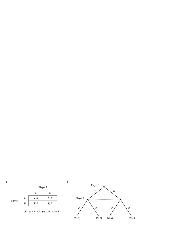
Figure 1: The strategic a) and extensive b) form of the Prisoner’s Dilemma.

It demonstrates why the rationality of players can lead them to an inefficient outcome. Although the payoff vector $(R,R)$ is better to both players than $(P,P)$, they cannot obtain this outcome since each player’s strategy $C$ (cooperation) is strictly dominated by $D$ (defection). As a result, the players end up with payoff $P$ corresponding to the unique Nash equilibrium $(D,D)$.

A similar scenario occurs in a case of finitely repeated PD. The concept of a finitely repeated game assumes playing a static game (a stage of the repeated game) for a fixed number of times. Additionally, the players are informed about results of consecutive stages. In the twice repeated case it means that each player’s strategy specify an action at the first stage and four actions at the second stage where a particular action is chosen depending on what of the four outcomes of the first stage has occurred. It is clearly visible when we write twice repeated game in the extensive form (see Fig. 2).

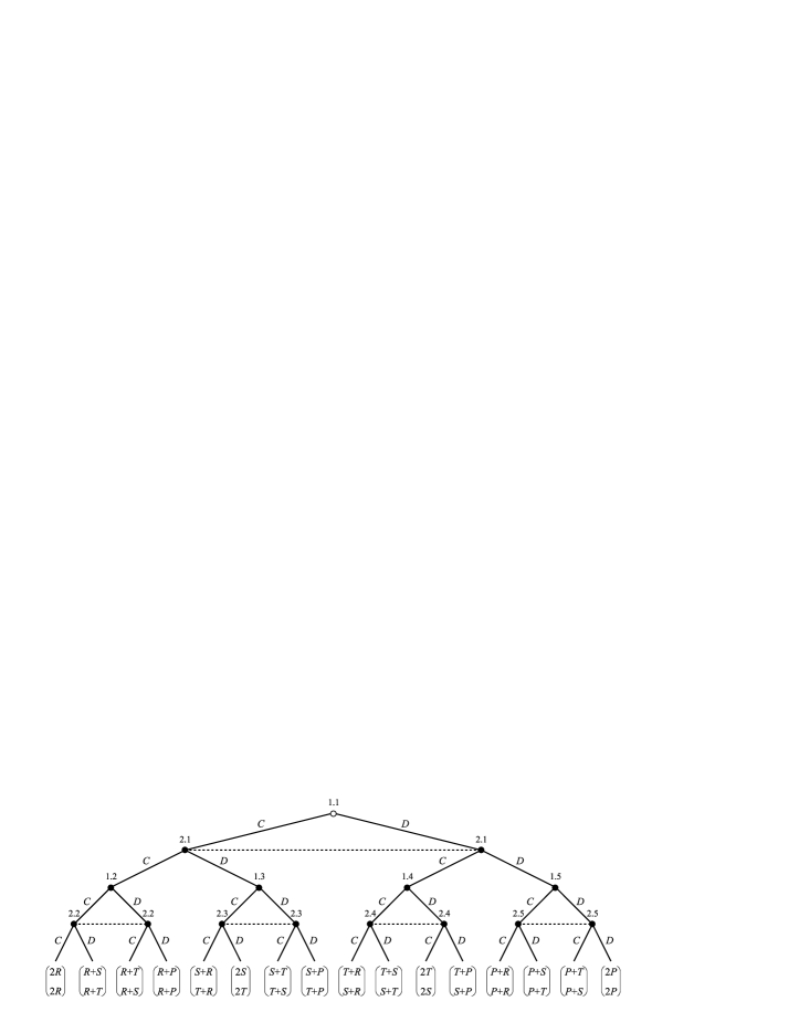
Figure 2: The extensive form for a twice repeated Prisoner Dilemma.

The first stage of the twice repeated PD in the extensive form is simply the game depicted in Fig. 1(b) where the players specify an action $C$ or $D$ at the information set 1.1 and 2.1, respectively (the information sets of player 2 are distinguished by dotted line connecting the nodes to show lack of knowledge of the second player about the previous move of the first player). When the players choose their actions, the result of the first stage is announced. Since they have knowledge about the results of the first stage, they can choose different actions at the second stage depending on the previous result, hence the next four game trees from Fig. 1 are required to describe the repeated game. The game tree exhibits ten information sets (five for each player labelled $1.\cdot$ and $2.\cdot$, respectively) at which each of the players has two moves. Thus, each of them has $2^{5}=32$ strategies as they specify $C$ or $D$ at their own five information sets.

To find the Nash equilibrium in finitely repeated game it is convenient to use the property that the equilibrium profile always implies the Nash equilibrium at the last stage of the game. Therefore, to find the Nash equilibrium in the twice repeated PD it is sufficient to consider strategy profiles that generate the profile $(D,D)$ at the second stage. Then it follows that $D$ is the best response for players at the first stage as well. By induction it can be shown that playing the action $D$ at each stage of finitely repeated PD constitutes the unique Nash equilibrium. It is worth noting that if a single stage of repeated game has more than one equilibrium, different Nash equilibria may be played at the last stage depending on results of previous stages. For example, let us consider the Battle of the Sexes (BoS) game given by the following bimatrix:

$$\begin{array}[]{l}~{}~{}~{}~{}~{}~{}~{}~{}~{}~{}~{}~{}~{}\quad O\qquad~{}~{}F\\ \Gamma:\begin{array}[]{c}O\\ F\end{array}\left[\begin{array}[]{cc}(\alpha,\beta)&(\gamma,\gamma)\\ (\gamma,\gamma)&(\beta,\alpha)\\ \end{array}\right],\quad$where$\quad\alpha>\beta>\gamma.\end{array}$$ (1)

It has two pure Nash equilibria, namely, $(O,O)$ and $(F,F)$. Let us examine now the twice repeated BoS. Obviously, its game tree is the same as one in Fig. 2. Let us assign appropriate sum of two stage payoff outcomes to each possible profile (like it has been done in the case of the twice repeated PD). Then we find many different Nash equilibria. One of these is to play the Nash equilibrium $(O,O)$ at the first stage, keep playing $(O,O)$ at the second stage if the outcome of the first one is $(O,O)$ or $(O,F)$, otherwise to play stage-game Nash equilibrium $(F,F)$.

3 Comment on ‘Quantum repeated games’ by Iqbal and Toor [2]

Let us remind the MW approach to playing the PD repeatedly introduced in [2]. According to this concept the two-stage PD is placed in $\mathscr{H}=\left(\mathds{C}^{2}\right)^{\otimes 4}$ complex Hilbert space with the computational basis. The game starts with preparing 4-qubit pure state represented by a unit vector in $\mathscr{H}$. The general form of this state is described as follows:

$$\begin{split}&|\psi_{\mathrm{in}}\rangle=\sum_{x_{1},x_{2},x_{3},x_{4}=0,1}\lambda_{x_{1},x_{2},x_{3},x_{4}}|x_{1},x_{2},x_{3},x_{4}\rangle,\\ &\mbox{where}\quad\lambda_{x_{1},x_{2},x_{3},x_{4}}\in\mathds{C}\quad\mbox{and}\quad\sum_{x_{1},x_{2},x_{3},x_{4}=0,1}|\lambda_{x_{1},x_{2},x_{3},x_{4}}|^{2}=1.\end{split}$$ (2)

Players’ moves are identified with the identity operator $\sigma_{0}$ and the bit flip Pauli operator $\sigma_{1}$. Player 1 is allowed to act on the first and third qubit, and player 2 acts on the second and fourth one. In the first stage of the game the two first qubits are manipulated. Let $\rho_{\mathrm{in}}$ be the density operator for the initial state (2). Then the state $\rho$ after the players’ actions takes the form

$$\begin{split}&\rho=\sum_{\kappa_{1},\kappa_{2}=0,1}p_{\kappa_{1}}q_{\kappa_{2}}(\sigma^{1}_{\kappa_{1}}\otimes\sigma^{2}_{\kappa_{2}})\rho_{\mathrm{in}}(\sigma^{1}_{\kappa_{1}}\otimes\sigma^{2}_{\kappa_{2}}),\\ &\mbox{and}\;\;\sum_{\kappa_{1}=0,1}p_{\kappa_{1}}=\sum_{\kappa_{2}=0,1}q_{\kappa_{2}}=1,\end{split}$$ (3)

where $p_{\kappa_{1}}$ ($q_{\kappa_{2}}$) is the probability of applying $\sigma^{1}_{\kappa_{1}}$ ($\sigma^{2}_{\kappa_{2}})$ to the first (second) qubit. Next, the other two qubits are manipulated which, according to Iqbal and Toor, corresponds to the second stage of the classical game. The operation $\sigma^{3}_{\kappa_{3}}$ on the third qubit with probability $p_{\kappa_{3}}$ and operation $\sigma^{4}_{\kappa_{4}}$ on the fourth qubit with probability $q_{\kappa_{4}}$ change the state $\rho$ to

$$\begin{split}&\rho_{\mathrm{fin}}=\sum_{\kappa_{3},\kappa_{4}=0,1}p_{\kappa_{3}}q_{\kappa_{4}}(\sigma^{3}_{\kappa_{3}}\otimes\sigma^{4}_{\kappa_{4}})\rho(\sigma^{3}_{\kappa_{3}}\otimes\sigma^{4}_{\kappa_{4}}),\\ &\mbox{and}\quad\;\;\sum_{\kappa_{3}=0,1}p_{\kappa_{3}}=\sum_{\kappa_{4}=0,1}q_{\kappa_{4}}=1.\end{split}$$ (4)

The next step is to measure the final state $\rho_{\mathrm{fin}}$ in order to determine final payoffs. The measurement is defined by the four payoffs operators $X_{i.j}$, $i,j=1,2$ associated with particular: player $i$ and stage $j$. That is

$$\begin{split}X_{1.1}=(R|00\rangle\langle 00|+S|01\rangle\langle 01|+T|10\rangle\langle 10|+P|11\rangle\langle 11|)\otimes\mathds{1}^{\otimes 2};\\ X_{1.2}=\mathds{1}^{\otimes 2}\otimes(R|00\rangle\langle 00|+S|01\rangle\langle 01|+T|10\rangle\langle 10|+P|11\rangle\langle 11|);\\ X_{2.1}=(R|00\rangle\langle 00|+T|01\rangle\langle 01|+S|10\rangle\langle 10|+P|11\rangle\langle 11|)\otimes\mathds{1}^{\otimes 2};\\ X_{2.2}=\mathds{1}^{\otimes 2}\otimes(R|00\rangle\langle 00|+T|01\rangle\langle 01|+S|10\rangle\langle 10|+P|11\rangle\langle 11|).\end{split}$$ (5)

Then the expected payoff $E_{i.j}$ for player $i$ at stage $j$ when player 1 chooses strategy $(\sigma^{1}_{\kappa_{1}},\sigma^{3}_{\kappa_{3}})$ and player 2 chooses $(\sigma^{2}_{\kappa_{2}},\sigma^{4}_{\kappa_{4}})$ is obtained by the following formula:

$$E_{i.j}\left((\sigma^{1}_{\kappa_{1}},\sigma^{3}_{\kappa_{3}}),(\sigma^{2}_{\kappa_{2}},\sigma^{4}_{\kappa_{4}})\right)=\mathrm{tr}(X_{i.j}\rho_{\mathrm{fin}}).$$ (6)

The authors took up the issue of cooperation in two-stage PD. Given the initial state

$$|\psi_{\mathrm{in}}\rangle=\lambda_{0000}|0000\rangle+\lambda_{0011}|0011\rangle+\lambda_{1100}|1100\rangle+\lambda_{1111}|1111\rangle$$ (7)

and fixed payoffs

$$T=5,\quad R=3,\quad P=1,\quad S=0,$$ (8)

they identify $\sigma_{0}$ and $\sigma_{1}$ as actions of cooperation and defection, respectively, and claim that conditions

$$|\lambda_{0000}|^{2}+|\lambda_{0011}|^{2}\leq\frac{1}{3},\quad|\lambda_{0011}|^{2}+|\lambda_{1111}|^{2}\leq\frac{1}{3}$$ (9)

are sufficient to choose $\sigma_{0}$ by both players (thereby cooperating) at the first stage given that the players have chosen $\sigma_{1}$ at the second one. We raise below two objections concerning the results of the paper [2].

3.1 The incompatibility of the protocol (2)-(6) and theory of repeated games

The main fault of the protocol (2)-(6) is that the twice repeated game cannot be described in this way. In fact, it quantizes the game PD played twice when the players are not informed about a result of the first stage. It is noticeable, for example, when we re-examine the way of finding the optimal solution provided in [2]. The authors analyze the game backwards, first by focusing on the Nash equilibria at the second stage. They set condition for the profile $(\sigma^{3}_{1},\sigma^{4}_{1})$ to be the Nash equilibrium at the second stage. Next, given that $(\sigma^{3}_{1},\sigma^{4}_{1})$ is fixed, they determine the set of amplitudes for which the profile $((\sigma^{1}_{0},\sigma^{2}_{0}),(\sigma^{3}_{1},\sigma^{4}_{1}))$ is the Nash equilibrium of the game implied by (2)-(6). This method to find the Nash equilibria is not correct since it doesn’t include the possibility that players make their actions depending on a result of the first stage. Although the problem seems to be insignificant where a stage of a repeated game has unique Nash equilibrium, it becomes visible in remaining cases. Let us consider the initial state (7) satisfying the requirement

$$2(|\lambda_{0000}|^{2}+|\lambda_{1100}|^{2})=|\lambda_{0011}|^{2}+|\lambda_{1111}|^{2}$$ (10)

and let us take (8) to be PD’s payoffs. Then, the expected payoffs for the players at the second stage of the game defined by the scheme (2)-(6) are as follows:

$$\begin{split}&E_{i.2}\bigl{(}(\cdot,\sigma^{3}_{0}),(\cdot,\sigma^{4}_{0})\bigr{)}=E_{1.2}\bigl{(}(\cdot,\sigma^{3}_{1}),(\cdot,\sigma^{4}_{0})\bigr{)}=E_{2.2}\bigl{(}(\cdot,\sigma^{3}_{0}),(\cdot,\sigma^{4}_{1})\bigr{)}=5|\lambda|;\\ &E_{1.2}\bigl{(}(\cdot,\sigma^{3}_{0}),(\cdot,\sigma^{4}_{1})\bigr{)}=E_{2.2}\bigl{(}(\cdot,\sigma^{3}_{1}),(\cdot,\sigma^{4}_{0})\bigr{)}=10|\lambda|;\\ &E_{i.2}\bigl{(}(\cdot,\sigma^{3}_{1}),(\cdot,\sigma^{4}_{1})\bigr{)}=7|\lambda|,\end{split}$$ (11)

where $|\lambda|=|\lambda_{0000}|^{2}+|\lambda_{1100}|^{2}$ and $i=1,2$. Results of (11) imply continuum of Nash equilibria in the second stage (it is easy to note, for example, when we draw a $2\times 2$ bimatrix with entries defined by (11)), among them $\left((\cdot,\sigma^{3}_{0}),(\cdot,\sigma^{4}_{1})\right)$ and $\left((\cdot,\sigma^{3}_{1}),(\cdot,\sigma^{4}_{0})\right)$. Bearing in mind the remark in Section 2 about possible profiles in the BoS game, the correct protocol for quantum repeated games should be able to assign a payoff outcome (by the measurement (5)) to a strategy profile, where different Nash equilibria are played at the second stage depending on actions chosen at the first one. However, an example of a profile where the players play $\left((\cdot,\sigma^{3}_{0}),(\cdot,\sigma^{4}_{1})\right)$ at the second stage if a result of the first stage is $\left((\sigma^{1}_{0},\cdot),(\sigma^{2}_{0},\cdot)\right)$, and they play $\left((\cdot,\sigma^{3}_{1}),(\cdot,\sigma^{4}_{0})\right)$ in other cases cannot be measured by the scheme (2)-(6). Since there is two qubit register allotted to the second stage, it allows to write only one pair of actions $(\sigma^{3}_{\kappa_{3}},\sigma^{4}_{\kappa_{4}})$ before the measurement is made.

An argument against the scheme in [2] can be expressed in another way. Namely, all results included in [2] can be obtained by considering simplified protocol (2)-(6) where the sequential procedure (3) and (4) for determining the final state $\rho_{\mathrm{fin}}$ is simply replaced with

$$\rho_{\mathrm{fin}}=\bigotimes^{4}_{j=1}\sigma^{j}_{\kappa_{j}}\rho_{\mathrm{in}}\bigotimes^{4}_{j=1}\sigma^{j}_{\kappa_{j}},$$ (12)

In this case, the first and the second player simultaneously pick $(\sigma^{1}_{\kappa_{1}},\sigma^{3}_{\kappa_{3}})$ and $(\sigma^{2}_{\kappa_{2}},\sigma^{4}_{\kappa_{4}})$, respectively, having essentially only four strategies each. However, as we mentioned in the previous section, each player has 32 strategies in the classical twice repeated game. As a result, the protocol (2)-(6) cannot coincide with the classical case if $|\psi_{\mathrm{in}}\rangle=|0000\rangle$. Despite the fact that the Authors assume that a player knows her opponent’s action taken previously, the scheme (2)-(6) does not take it into consideration. In consequence, a game being quantized by (2)-(6) differs from the game in Fig. 2 in that the nodes 1.2, 1.3, 1.4 and 1.5 (2.2, 2.3, 2.4 and 2.5) lie at the same information set (are connected with dotted line).

3.2 The misconception about the cooperative strategy in the PD played via the MW approach

The another fault, we are going to discuss, is based on misinterpreting the operators $\sigma_{0}$ and $\sigma_{1}$ as cooperation and defection in the protocol given by (2)-(6). Let us consider the initial state $|\psi_{\mathrm{in}}\rangle$ where the two first qubits associated with the first stage are prepared in the state $|x_{1},x_{2}\rangle$, for $x_{1},x_{2}\in\{0,1\}$. Then the first stage of the game given by (2)-(6) is isomorphic to the classical PD game. When the initial state is $|00\rangle$ then $\sigma_{0}$ corresponds to the action $C$ and $\sigma_{1}$ corresponds to $D$. However, when the initial state is $|11\rangle$, the action ‘cooperate’ are identified with $\sigma_{1}$ and the action ‘defect’ with $\sigma_{0}$ since by putting $\rho_{\mathrm{fin}}=(\sigma^{1}_{\kappa_{1}}\otimes\sigma^{2}_{\kappa_{2}})|11\rangle\langle 11|(\sigma^{1}_{\kappa_{1}}\otimes\sigma^{2}_{\kappa_{2}})$ into the formula (6) we have

$$(\mathrm{tr}(X_{1.1}\rho_{\mathrm{fin}}),\mathrm{tr}(X_{2.1}\rho_{\mathrm{fin}}))=\left\{\begin{array}[]{lll}(R,R),&\mbox{if}&(\kappa_{1},\kappa_{2})=(1,1);\\ (S,T),&\mbox{if}&(\kappa_{1},\kappa_{2})=(1,0);\\ (T,S),&\mbox{if}&(\kappa_{1},\kappa_{2})=(0,1);\\ (P,P),&\mbox{if}&(\kappa_{1},\kappa_{2})=(0,0).\end{array}\right.$$ (17)

That is, the outcome of the game does not depend intrinsically on the operators but depends on the initial state and on what the final state $\rho_{\mathrm{fin}}$ can be obtained through the available operators. Thus identification of operators with actions taken in classical game without taking into consideration the form of the initial state is not correct. The misidentification assumed in [2] implies that the condition (9) cannot solve the problem formulated in this paper. It is clearly visible when we take, for example, the initial state $|\psi_{\mathrm{in}}\rangle=|1100\rangle$. It satisfies the inequalities (9) thus, $\sigma_{0}$ is optimal at the first stage for each player. In fact, $\sigma_{0}$ is the action ‘defect’ as it is shown in (17). Note also that the payoff corresponding to the profile $(\sigma_{0},\sigma_{0})$ at the first stage and $(\sigma_{1},\sigma_{1})$ at the second one is $2P$ for each player - total payoff for the defection. Thus, the condition (9) does not ensure the cooperation at the first stage.

Quite the opposite, it turns out that the players never cooperate when they play the game defined by (2)-(6). Let us consider any initial state (2) in which the first and the second qubit are prepared in a way that for $(s_{1},s_{2})=((\sigma^{1}_{\kappa_{1}},\sigma^{3}_{\kappa_{3}}),(\sigma^{2}_{\kappa_{2}},\sigma^{4}_{\kappa_{4}}))$ we have

$$(E_{1.1}(s_{1},s_{2}),E_{2.1}(s_{1},s_{2}))=\left\{\begin{array}[]{lll}(R^{\prime},R^{\prime}),&\mbox{if}&(\kappa_{1},\kappa_{2})=(0,0);\\ (S^{\prime},T^{\prime}),&\mbox{if}&(\kappa_{1},\kappa_{2})=(0,1);\\ (T^{\prime},S^{\prime}),&\mbox{if}&(\kappa_{1},\kappa_{2})=(1,0);\\ (P^{\prime},P^{\prime}),&\mbox{if}&(\kappa_{1},\kappa_{2})=(1,1).\end{array}\right.$$ (22)

where the values $T^{\prime},R^{\prime},P^{\prime},S^{\prime}$ meet the requirements of the PD given in Fig.1(a), so the operators $\sigma_{0}$ and $\sigma_{1}$ can be regarded as cooperation and defection, respectively. Next, let us estimate the difference

$$E_{1}((\sigma^{1}_{1},\sigma^{3}_{0}),s_{2})-E_{1}((\sigma^{1}_{0},\sigma^{3}_{0}),s_{2})\quad\mbox{for any}\quad s_{2}=(\sigma^{2}_{\kappa_{2}},\sigma^{4}_{\kappa_{4}}),$$ (23)

where $E_{1}=E_{1.1}+E_{1.2}$. Since the same actions are taken on the third and the fourth qubit, we have $E_{1.2}((\sigma^{1}_{0},\sigma^{3}_{0}),s_{2})=E_{1.2}((\sigma^{1}_{1},\sigma^{3}_{0}),s_{2})$, therefore, the value $E_{1}$ depends only on $E_{1.1}$, Thus, for $s_{2}=(\sigma^{2}_{\kappa_{2}},\sigma^{4}_{\kappa_{4}})$, we obtain from (22) that

$$0<E_{1}((\sigma^{1}_{1},\sigma^{3}_{0}),s_{2})-E_{1}((\sigma^{1}_{0},\sigma^{3}_{0}),s_{2})=\left\{\begin{array}[]{lll}T^{\prime}-R^{\prime},&\mbox{if}&\kappa_{2}=0;\\ P^{\prime}-S^{\prime},&\mbox{if}&\kappa_{2}=1.\end{array}\right.$$ (26)

In similar way we can prove that the strategy $(\sigma^{1}_{0},\sigma^{3}_{1})$ of player 1 is strictly dominated by $(\sigma^{1}_{1},\sigma^{3}_{1})$. As a result, we conclude that $\sigma^{1}_{1}$ is the best response of player 1 at the first stage. Symmetry of payoffs in PD implies that strategy $(\sigma^{2}_{0},\sigma^{4}_{0})$ of player 2 is strictly dominated by $(\sigma^{2}_{1},\sigma^{4}_{0})$, as well as $(\sigma^{2}_{0},\sigma^{4}_{1})$ is strictly dominated by $(\sigma^{2}_{1},\sigma^{4}_{1})$. Thus, there is no Nash equilibrium in which the players choose $\sigma_{0}$ (cooperation) at the first stage.

4 The MW approach to twice repeated quantum games

In this section we propose a scheme of playing a twice repeated $2\times 2$ quantum game that is free from the faults we have pointed in the previous section. Our construction is based on the protocol that we proposed in [5] where general finite extensive quantum games were considered. Since a repeated game is a special case of an extensive game, we can adapt this concept. Next, we examine what results can be obtained from such protocol. In particular, we re-examine the problem of cooperation studied in [2].

4.1 Construction of a twice repeated $\mathbf{2\times 2}$ quantum game via the MW protocol

Let us consider a $2\times 2$ game defined by the outcomes $O_{\iota_{1},\iota_{2}}$, $\iota_{1},\iota_{2}=0,1$. The twice repeated $2\times 2$ quantum game played according to the MW approach is as follows:

Let $\mathscr{H}=\left(\mathds{C}^{2}\right)^{\otimes 10}$ be a Hilbert space with the computational basis $\{|x_{1},x_{2},\dots,x_{10}\rangle\}$, $x_{j}=0,1$. Then the initial state of the game is a ten-qubit pure state represented by a unit vector in the space $\mathscr{H}$:

$$|\psi_{\mathrm{in}}\rangle=\sum^{2^{10}-1}_{x=0}\lambda_{x}|x\rangle,\quad\mbox{for}\quad\lambda_{x}\in\mathds{C}\quad\mbox{and}\quad\sum_{x}|\lambda_{x}|^{2}=1,$$ (27)

where the sum is over all possible decimal values of $x=(x)_{10}=(x_{1}x_{2}\dots x_{10})_{2}$. The players are allowed to apply operators $\sigma_{0}$ and $\sigma_{1}$. The qubits with odd indices are manipulated by player 1 and the qubits labelled by even indices are manipulated by player 2. Such assignment implies 32 possible strategies for each players as they specify five operations $\sigma^{j}_{\kappa_{j}}$ (where $j$ and $\kappa_{j}$ indicate qubit number and operation number, respectively) on their own qubits. We denote a player $i$’s strategy by $\tau_{i}=(\sigma^{i}_{\kappa_{i}},\sigma^{i+2}_{\kappa_{i+2}},\sigma^{i+4}_{\kappa_{i+4}},\sigma^{i+6}_{\kappa_{i+6}},\sigma^{i+8}_{\kappa_{i+8}}),$ where $i=1,2$. The profile $\tau=(\tau_{1},\tau_{2})$ gives rise to the final state:

$$|\psi_{\mathrm{fin}}\rangle=\bigotimes^{10}_{j=1}\sigma^{j}_{\kappa_{j}}|\psi_{\mathrm{in}}\rangle.$$ (28)

If the players each take $\tau^{t}_{1}$ and $\tau^{t^{\prime}}_{2}$ with probability $p_{t}$ and $q_{t^{\prime}}$, respectively, that corresponds to the state $|\psi_{\mathrm{fin}}^{t,t^{\prime}}\rangle$ (defined by (28)) with probability $p_{t}q_{t^{\prime}}$, then the final state is the density operator associated with the ensemble $\{p_{t}q_{t^{\prime}},|\psi_{\mathrm{fin}}^{t,t^{\prime}}\rangle\}$. That is

$$\rho_{\mathrm{fin}}=\sum_{t,t^{\prime}}p_{t}q_{t^{\prime}}|\psi_{\mathrm{fin}}^{t,t^{\prime}}\rangle\langle\psi_{\mathrm{fin}}^{t,t^{\prime}}|.$$ (29)

Till now, a difference between the concept in [2] and our protocol lies in the dimension of the space $\mathscr{H}$. The next difference is clearly visible in a description of measurement operators. The measurement on $\rho_{\mathrm{fin}}$ that determines an outcome of the game is described by a collection $\{X_{1},X_{2.00},X_{2.01},X_{2.10},X_{2.11}\}$, where its components are defined as follows:

$$X_{1} =\sum_{x_{1},x_{2}\in\{0,1\}}O_{x_{1},x_{2}}|x_{1},x_{2}\rangle\langle x_{1},x_{2}|\otimes\mathds{1}^{\otimes 8};$$ (30)

$$\begin{split}X_{2.00}&=\sum_{x_{3},x_{4}\in\{0,1\}}O_{x_{3},x_{4}}|00\rangle\langle 00|\otimes|x_{3},x_{4}\rangle\langle x_{3},x_{4}|\otimes\mathds{1}^{\otimes 6};\\ X_{2.01}&=\sum_{x_{5},x_{6}\in\{0,1\}}O_{x_{5},x_{6}}|01\rangle\langle 01|\otimes\mathds{1}^{\otimes 2}\otimes|x_{5},x_{6}\rangle\langle x_{5},x_{6}|\otimes\mathds{1}^{\otimes 4};\\ X_{2.10}&=\sum_{x_{7},x_{8}\in\{0,1\}}O_{x_{7},x_{8}}|10\rangle\langle 10|\otimes\mathds{1}^{\otimes 4}\otimes|x_{7},x_{8}\rangle\langle x_{7},x_{8}|\otimes\mathds{1}^{\otimes 2};\\ X_{2.11}&=\sum_{x_{9},x_{10}\in\{0,1\}}O_{x_{9},x_{10}}|11\rangle\langle 11|\otimes\mathds{1}^{\otimes 6}\otimes|x_{9},x_{10}\rangle\langle x_{9},x_{10}|.\end{split}$$ (31)

Then the expected outcomes: $E_{i.1}$ at the first stage and $E_{i.2}$ at the second stage are calculated by using the following formulae:

$$E_{i.1}=\mathrm{tr}(X_{1}\rho_{\mathrm{fin}}),\quad E_{i.2}=\mathrm{tr}\left(\sum_{\iota_{1},\iota_{2}}X_{2.\iota_{1},\iota_{2}}\rho_{\mathrm{fin}}\right).$$ (32)

Let us give justification of our construction. Notice that $2^{10}$ is a minimal dimension of the space $\mathscr{H}$ in order to play the twice repeated $2\times 2$ game. Since a player’s strategy in a twice repeated $2\times 2$ game specifies action at the first stage and at each of four subgames fixed by the outcome of the first stage, the quantum protocol needs a five-qubit register to write a player’s strategy. The first two qubits are used to perform operations at the first stage of the repeated game. Then given the form of $X_{1}$ and strategies of players restricted to manipulate the first and the second qubit, in fact, the protocol (27)-(32) coincides with the MW scheme of playing $2\times 2$ quantum game [1]. The remaining eight qubits are used to define players’ moves at the second stage. That is, by pairing consecutive qubits from the third qubit onwards, actions at the second stage are defined on appropriate pair of qubits depending on the outcome at the previous stage. For example, given the outcome $O_{10}$ has occurred at the first stage (that is the outcome 10 on the first two qubits has been measured), the expected outcome $E_{i.2}$ depends only on operation on $x_{7}$ and $x_{8}$, i.e, $E_{i.2}=\mathrm{tr}(X_{2.10}\rho_{\mathrm{fin}})$. Then the players play the second stage in the same way as in the protocol (2)-(6). However, contrary to the previous idea, each player specifies her move for each possible outcome $O_{x_{1},x_{2}}$.

A game generated by our scheme naturally coincides with the classical case when appropriate initial state is prepared. We prove this fact by means of a convenient sequential approach to (27)-(32) provided in the next section.

4.2 Extensive form of a quantum twice repeated $\mathbf{2\times 2}$ game

The protocol (27)-(32) allows to put a game into an extensive form by using a similar method to what was described in [5]. The extensive form is obtained through sequential calculating the final state $\rho_{\mathrm{fin}}$ according to the following procedure. At first the players manipulate the first pair of qubits. Then the measurement in the computational basis is made on these qubits (as a result, an outcome $O_{\iota_{1},\iota_{2}}$ of the first stage is returned). The measured outcome is sent to the players. Depending on the measurement outcome $\iota_{1},\iota_{2}$ that occurs with probability $p(\iota_{1},\iota_{2})$ the players act on the next pair of qubits: if $\iota_{1},\iota_{2}$ is observed then player 1 and player 2 manipulate qubits $2\iota+3$ and $2\iota+4$, respectively, where $\iota=(\iota_{1}\iota_{2})_{2}$ is a decimal representation of a binary number $\iota_{1}\iota_{2}$. The procedure can be formally described as follows:

Algoritm 4.1

1.	$(\sigma^{1}_{\kappa_{1}}\otimes\sigma^{2}_{\kappa_{2}})|\psi_{\mathrm{in}}\rangle=|\psi\rangle$		The players perform their operations $\sigma^{1}_{\kappa_{1}}$ and $\sigma^{2}_{\kappa_{2}}$ on the initial state $|\psi_{\mathrm{in}}\rangle$.
2.	$\to\displaystyle\frac{M_{\iota_{1},\iota_{2}}|\psi\rangle}{\sqrt{\langle\psi|M_{\iota_{1},\iota_{2}}|\psi\rangle}}=|\psi_{\iota_{1},\iota_{2}}\rangle$		The first two qubits in the state $\rho$ are measured. The measurement is described by a collection $\{M_{\iota_{1},\iota_{2}}\colon M_{\iota_{1},\iota_{2}}=|\iota_{1},\iota_{2}\rangle\langle\iota_{1},\iota_{2}|\otimes\mathds{1}^{\otimes 8},\iota_{1},\iota_{2}=0,1\}$.
3.	$\to\{p(\iota_{1},\iota_{2}),(\sigma^{2\iota+3}_{\kappa_{2\iota+3}}~{}\otimes~{}\sigma^{2\iota+4}_{\kappa_{2\iota+4}})|\psi_{\iota_{1},\iota_{2}}\rangle\}$ $~{}~{}~{}~{}~{}~{}~{}p(\iota_{1},\iota_{2})=\langle\psi|M_{\iota_{1},\iota_{2}}|\psi\rangle$		Given that the outcome $\iota_{1},\iota_{2}$ has been observed, players 1 and 2 perform operations $\sigma^{2\iota+3}_{\kappa_{2\iota+3}}$ and $\sigma^{2\iota+4}_{\kappa_{2\iota+4}}$ on the post-measurement state.

It turns out that we can prove

Proposition 4.2

The density operator $|\psi_{\mathrm{fin}}\rangle\langle\psi_{\mathrm{fin}}|$ associated with state (28) and the density operator for the ensemble $\{p(\iota_{1},\iota_{2}),(\sigma^{2\iota+3}_{\kappa_{2\iota+3}}\otimes\sigma^{2\iota+4}_{\kappa_{2\iota+4}})|\psi_{\iota_{1},\iota_{2}}\rangle\}$ in Algorithm 4.1 determine the same outcomes $E_{i.1}$ and $E_{i.2}$ with regard to the measurement (30)–(31).

Proof. Let us put $\rho=|\psi\rangle\langle\psi|$. Given that $|\psi_{\iota_{1},\iota_{2}}\rangle\langle\psi_{\iota_{1},\iota_{2}}|=M_{\iota_{1},\iota_{2}}\rho M_{\iota_{1},\iota_{2}}/p(\iota_{1},\iota_{2})$ the state $\rho^{\prime}_{\mathrm{fin}}$ can be written as:

$$\rho^{\prime}_{\mathrm{fin}}=\sum_{\iota_{1},\iota_{2}=0,1}\sigma^{2\iota+3}_{\kappa_{2\iota+3}}\otimes\sigma^{2\iota+4}_{\kappa_{2\iota+4}}M_{\iota_{1},\iota_{2}}\rho M_{\iota_{1},\iota_{2}}\sigma^{2\iota+3}_{\kappa_{2\iota+3}}\otimes\sigma^{2\iota+4}_{\kappa_{2\iota+4}}.$$ (33)

Since the first and the second qubits are measured, any operation $\sigma^{j}_{\kappa_{j}}$ for which $j\neq 1,2$ does not influence the measurement. Therefore we have

$$\rho^{\prime}_{\mathrm{fin}}=\sum_{\iota_{1},\iota_{2}=0,1}M_{\iota_{1},\iota_{2}}\sigma^{2\iota+3}_{\kappa_{2\iota+3}}\otimes\sigma^{2\iota+4}_{\kappa_{2\iota+4}}\rho\,\sigma^{2\iota+3}_{\kappa_{2\iota+3}}\otimes\sigma^{2\iota+4}_{\kappa_{2\iota+4}}M_{\iota_{1},\iota_{2}}.$$ (34)

Note that $X_{\iota^{\prime}_{1},\iota^{\prime}_{2}}M_{\iota_{1},\iota_{2}}=\delta_{\iota,\iota^{\prime}}X_{\iota^{\prime}_{1},\iota^{\prime}_{2}}$, where $\delta_{\iota,\iota^{\prime}}$ is the Kronecker’s delta, and $\iota=(\iota_{1},\iota_{2})_{2}$, and $\iota^{\prime}=(\iota^{\prime}_{1},\iota^{\prime}_{2})_{2}$, Using the form (34) of $\rho^{\prime}_{\mathrm{fin}}$ we have

$$\mathrm{tr}\left(\sum_{\iota^{\prime}}X_{2.\iota^{\prime}_{1},\iota^{\prime}_{2}}\rho^{\prime}_{\mathrm{fin}}\right)=\mathrm{tr}\left(\sum_{\iota}X_{2.\iota_{1},\iota_{2}}\sigma^{2\iota+3}_{\kappa_{2\iota+3}}\otimes\sigma^{2\iota+4}_{\kappa_{2\iota+4}}\rho\sigma^{2\iota+3}_{\kappa_{2\iota+3}}\otimes\sigma^{2\iota+4}_{\kappa_{2\iota+4}}\right).$$ (35)

For each $\iota$ the trace of each term of the sum on the right-hand side of equation (35) depends only on an operation $\sigma^{j}_{\kappa_{j}}$ on a qubit $j$, where $j\in\{1,2,2\iota+3,2\iota+4\}$. Thus, the equation (35) holds when also the rest of operations $\sigma^{j}_{\kappa_{j}}$ are added:

$$\mathrm{tr}\left(\sum_{\iota}X_{2.\iota_{1},\iota_{2}}\rho^{\prime}_{\mathrm{fin}}\right)=\mathrm{tr}\left(\sum_{\iota}X_{2.\iota_{1},\iota_{2}}\bigotimes^{10}_{j=1}\sigma^{j}_{\kappa_{j}}\rho_{\mathrm{in}}\bigotimes^{10}_{j=1}\sigma^{j}_{\kappa_{j}}\right).$$ (36)

As a result, the left-hand side of (36) is equal to the expected outcome $E_{i.2}$ associated with the final state $|\psi_{\mathrm{fin}}\rangle\langle\psi_{\mathrm{fin}}|$. To prove that $\rho^{\prime}_{\mathrm{fin}}$ also determines the expected outcome $E_{i.1}$ let us see that $X_{1}$ and $\{M_{\iota_{1},\iota_{2}}\}$ are the same projective measurement up to the eigenvalues. Hence

$$\mathrm{tr}\left(X_{1}\rho^{\prime}_{\mathrm{fin}}\right)=\mathrm{tr}\left(X_{1}\sigma^{2\iota+3}_{\kappa_{2\iota+3}}\otimes\sigma^{2\iota+4}_{\kappa_{2\iota+4}}\rho\sigma^{2\iota+3}_{\kappa_{2\iota+3}}\otimes\sigma^{2\iota+4}_{\kappa_{2\iota+4}}\right).$$ (37)

Since $\rho=\sigma^{1}_{\kappa_{1}}\otimes\sigma^{2}_{\kappa_{2}}\rho_{\mathrm{in}}\sigma^{1}_{\kappa_{1}}\otimes\sigma^{2}_{\kappa_{2}}$, we obtain

$$\mathrm{tr}\left(X_{1}\rho^{\prime}_{\mathrm{fin}}\right)=\mathrm{tr}\left(X_{1}\bigotimes^{10}_{j=1}\sigma^{j}_{\kappa_{j}}\rho_{\mathrm{in}}\bigotimes^{10}_{j=1}\sigma^{j}_{\kappa_{j}}\right).$$ (38)

Equations (36) and (38) show that the state determined by the sequential procedure and state (28) set the same outcomes $E_{i.1}$ and $E_{i.2}$ for $i=1,2$. Using the same way as above and the linearity of the trace it can be proved that the equivalence is true if the players pick nondegenerate mixed strategies as well. $\square$

Having a sequential approach that is in conformity with protocol (27)-(32) we are able to analyze a quantum repeated game through an extensive form. It can facilitate the work significantly bearing in mind $32\times 32$ bimatrix associated with the normal representation of twice repeated $2\times 2$ game. Let us study the game tree drawn from the sequential procedure if the initial state (27) takes the form

$$|\psi_{\mathrm{in}}\rangle=\lambda_{0}|0\rangle^{\otimes 10}+\lambda_{1}|1\rangle^{\otimes 10}.$$ (39)

Let us use the sequential procedure step by step. At first the players manipulate $\sigma^{1}_{\kappa_{1}}$ and $\sigma^{2}_{\kappa_{2}}$. Hence we obtain the following state:

$$\sigma^{1}_{\kappa_{1}}\otimes\sigma^{2}_{\kappa_{2}}|\psi_{\mathrm{in}}\rangle=\lambda_{0}|\kappa_{1},\kappa_{2}\rangle|0\rangle^{\otimes 8}+\lambda_{1}|\overline{\kappa}_{1},\overline{\kappa}_{2}\rangle|1\rangle^{\otimes 8},$$ (40)

where $\overline{\kappa}_{j}$ is the negation of $\kappa_{j}$. A game tree at this phase is just the game tree corresponding to a $2\times 2$ game (see Fig. 1(b)), where $\sigma^{j}_{\kappa_{j}}$ for $j=1,2$, $\kappa_{j}=0,1$ are associated with respective branches of that game tree. After a sequence of actions $(\sigma^{1}_{\kappa_{1}},\sigma^{2}_{\kappa_{2}})$ the measurement $\{M_{\iota_{1},\iota_{2}}\}$ is made. Let us focus on the cases when the measurement outcome 00 or 11 has been observed. The form of (40) tells us that the measurement outcomes 00 and 11 are possible only if the profile at the first stage takes the form of $(\sigma^{1}_{\kappa},\sigma^{2}_{\kappa})$, where $\kappa=0,1$. Then, the probability $p(00)$ ($p(11)$) that the measurement outcome 00 (11) will occur is equal to $|\lambda_{\kappa}|^{2}$ ($|\lambda_{\overline{\kappa}}|^{2}$). Thus, the game tree is extended to include random actions 00 and 11 with associated probabilities after the both histories $(\sigma^{1}_{\kappa},\sigma^{2}_{\kappa})$. Since further moves of the players depend only on the measurement, the pair of histories $(\sigma^{1}_{0},\sigma^{2}_{0},00)$, $(\sigma^{1}_{1},\sigma^{2}_{1},00)$ and the pair $(\sigma^{1}_{0},\sigma^{2}_{0},11)$, $(\sigma^{1}_{1},\sigma^{2}_{1},11)$ constitute two separate information sets. Next, given that 00 (11) has occurred, following the sequential procedure, the players manipulate third and fourth (ninth and tenth) qubit at the second stage. Therefore another extensive form of $2\times 2$ is added to each sequence $(\sigma^{1}_{\kappa},\sigma^{2}_{\kappa},\iota\iota)$, where $\kappa,\iota=0,1$. In consequence we obtain a game tree shown in Fig. 3 (a part of the game tree after histories of $(\sigma^{1}_{\kappa},\sigma^{2}_{\overline{\kappa}})$, $\kappa=0,1$ is similar).

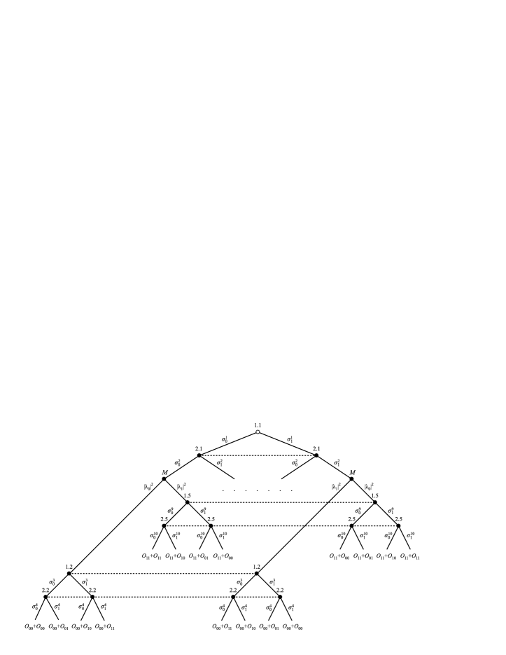
Figure 3: The extensive form for a twice repeated Prisoner Dilemma played through protocol (27)-(32) when the initial state is on the form of (39).

Each outcome associated with a terminal sequence are determined by a pure state from the ensemble given by the sequential procedure. For example, after sequence $(\sigma^{1}_{1},\sigma^{2}_{1})$ the post-measurement state takes the form of $|0\rangle^{\otimes 2}|1\rangle^{\otimes 8}$ (up to a global phase factor) with probability $|\lambda_{1}|^{2}$, and the players choose sequence $(\sigma^{3}_{\kappa_{3}},\sigma^{4}_{\kappa_{4}})$. Then the total outcome $E_{i}\mathrel{\mathop{:}}=E_{i.1}+E_{i.2}$ associated with a sequence $(\sigma^{1}_{1},\sigma^{2}_{1},00,\sigma^{3}_{\kappa_{3}},\sigma^{4}_{\kappa_{4}})$ is calculated according to formulae (32):

$$E_{i}=\mathrm{tr}\left(\left(X_{1}+\sum_{\iota_{1},\iota_{2}}X_{2.\iota_{1},\iota_{2}}\right)(|0\rangle\langle 0|)^{\otimes 2}|\overline{\kappa}_{3},\overline{\kappa}_{4}\rangle\langle\overline{\kappa}_{3},\overline{\kappa}_{4}|(|1\rangle\langle 1|)^{\otimes 6}\right).$$ (41)

The extensive approach allows us to see directly that our scheme coincides with the classical twice repeated $2\times 2$ game when $|\psi_{\mathrm{in}}\rangle=|0\rangle^{\otimes 10}$. Without loss of generality, let the outcomes $O_{\iota_{1},\iota_{2}}$ be the payoff outcomes corresponding to the PD game. Then putting $|\lambda_{0}|^{2}=1$ in (39) and assuming $\sigma^{j}_{0}\mathrel{\mathop{:}}=C$, $\sigma^{j}_{1}\mathrel{\mathop{:}}=D$ the game in Fig. 3 depicts exactly the classical twice repeated PD game (compare Fig. 2 and Fig. 3).

4.3 Twice repeated PD game played by means of the protocol (27)-(32)

Let us study the twice repeated PD game played with the use of our scheme. Analysis of our protocol with the general form initial state (27) is a laborious task and it deserves a separate paper to report about. Nevertheless, we can derive many interesting features with less effort considering the initial state of the form

$$|\psi_{\mathrm{in}}\rangle=\bigotimes^{5}_{j=1}|\varphi_{j}\rangle,\;\mbox{where}\;|\varphi_{j}\rangle\;\mbox{is a state of $2j-1$ and $2j$ qubit}.$$ (42)

Let us consider first the problem of optimization of the equilibrium payoffs, given a space of initial states as a domain.

Proposition 4.3

There are infinitely many settings of the initial state (27) for which the twice repeated PD game played with the use of the protocol (27)-(32) has a unique subgame perfect equilibrium with the equilibrium payoff $(2Q,2Q)$ such that $Q>P$.

Proof. Let us put the initial state (42) into the protocol (27)-(32) assuming that $|\varphi_{j}\rangle=|\varphi\rangle$ for any $j$. Then, the measurement $\{M_{\iota_{1},\iota_{2}}\}$ on the first pair of qubits does affect others qubits. Moreover, given that the outcome $O_{\iota_{1},\iota_{2}}$ has occurred, the expected outcome $E_{i.2}$ depends only on manipulating on one pair of qubits $|\varphi\rangle$ due to the form of (31). Therefore, regardless of the first stage outcome $O_{\iota_{1},\iota_{2}}$, the players are faced with a $2\times 2$ quantum game at the second stage (played via the MW approach). That is, the players are faced with the problem

$$\left(|\varphi\rangle\langle\varphi|,\{\sigma_{0},\sigma_{1}\},X^{\prime}_{i}\right),$$ (43)

where player 1 and 2 apply operators from the set $\{\sigma_{0},\sigma_{1}\}$ on the first and the second qubit of $|\varphi\rangle$, respectively. The outcome operator $X^{\prime}_{i}$ takes the form

$$X^{\prime}_{i}=\sum_{y_{1},y_{2}=0,1}O_{y_{1},y_{2}}|y_{1},y_{2}\rangle\langle y_{1},y_{2}|,$$ (44)

and the expected outcome is equal to

$$E_{i}(\sigma^{1}_{\kappa_{1}},\sigma^{2}_{\kappa_{2}})=\mathrm{tr}\left(\sigma^{1}_{\kappa_{1}}\otimes\sigma^{2}_{\kappa_{2}}|\varphi\rangle\langle\varphi|\sigma^{1}_{\kappa_{1}}\otimes\sigma^{2}_{\kappa_{2}}X^{\prime}_{i}\right).$$ (45)

Obviously, the first stage game is also described exactly as the triple (43). Since a quantum game according to the MW approach is a game expressed by a bimatrix, it leads us to the conclusion that protocol (27)-(32) with the initial state $|\varphi\rangle^{\otimes 5}$, in fact, can be treated as a twice repeated bimatrix game generated by (43).

Let us substitute $O_{y_{1},y_{2}}$ for the payoffs of the PD game in the game (43) and examine it towards uniqueness of Nash equilibria. Putting a state $|\varphi\rangle=\lambda_{0}|00\rangle+\lambda_{1}|11\rangle$, for which the amplitudes of $|\varphi\rangle$ satisfy the condition:

$$0<|\lambda_{0}|^{2}<\frac{\min\{T-R,P-S\}}{T-R+P-S}$$ (46)

the inequalities

$$E_{1}\left(\sigma^{1}_{0},\sigma^{2}_{\kappa_{2}}\right)>E_{1}\left(\sigma^{1}_{1},\sigma^{2}_{\kappa_{2}}\right)\quad\mbox{and}\quad E_{2}\left(\sigma^{1}_{\kappa_{1}},\sigma^{2}_{0}\right)>E_{1}\left(\sigma^{1}_{\kappa_{1}},\sigma^{2}_{1}\right)$$ (47)

are true for any $\kappa_{1},\kappa_{2}=0,1$. Inequalities (47) imply the unique Nash equilibrium $(\sigma^{1}_{0},\sigma^{2}_{0})$. Moreover, the first inequality of condition (46) ensures that

$$E_{1}\left(\sigma^{1}_{0},\sigma^{2}_{0}\right)=|\lambda_{0}|^{2}R+|\lambda_{1}|^{2}P>P.$$ (48)

Since the game constructed in the proof can be regarded as a classical twice repeated game, we are allowed to use all facts of classical repeated game theory. One of these tells us that a unique stage-game Nash equilibrium implies, for any finite number of repetitions, a unique subgame perfect equilibrium in which the stage-game Nash equilibrium is played in every stage. This completes the proof. $\square$

Of course, the protocol (27)-(32) can be re-formulated for any finitely repeated $2\times 2$ game and then statement analogical to Proposition 4.3 can be articulated. Unfortunately, the number of qubits required in our protocol grows exponentially with number of stages. For example, in the case of a game repeated three times, the protocol (27)-(32) needs next 32 qubits to describe the third stage. In general, the number of $\sum^{n}_{j=1}2^{2j-1}$ qubits is required for a $2\times 2$ game repeated $n$ times.

We shall re-examine now the problem of cooperation considered in [2]. We demonstrated in Section 3 that the cooperation at the first stage is not possible in the game defined by the Iqbal and Toor scheme. However, we also showed that this protocol does not take into consideration a player’s move at the second stage as a function of the first stage result. Therefore, in fact it does not allow to study the cooperation problem in a proper way. The following example proves that the cooperation of players is possible if the twice repeated PD game is played via our scheme.

Example 4.4

Let us set the PD game with payoff vectors

$$O_{00}=(4,4),\;O_{01}=(0,5),\;O_{10}=(5,0),\;O_{11}=(1,1)$$ (49)

inserted in (30) and (31). Let us also assume that the initial state (27) takes the form

$$|\psi_{\mathrm{in}}\rangle=|0\rangle^{\otimes 2}\left(\sqrt{0,6}|0\rangle^{\otimes 2}+\sqrt{0,4}|1\rangle^{\otimes 2}\right)|0\rangle^{\otimes 6}.$$ (50)

A game specified in this way differs from the classical one only in the subgame following the outcome $O_{00}$ of the first stage because then $E_{i.2}$ depends on operations on entangled third and fourth qubit. Since two first qubits in the state $|00\rangle$ imply the classical PD game at the first stage, we are permitted to identify the action ‘cooperate’ and the action ‘defect’ with $\sigma_{0}$ and $\sigma_{1}$, respectively, assuming $C\mathrel{\mathop{:}}=\sigma_{0}$ and $D\mathrel{\mathop{:}}=\sigma_{1}$. Moreover, the quantum measurement after the first stage is trivialized in this case and it coincides with the classical observation in an extensive game. It follows that both the game defined by (27)-(32), (49), (50) and the classical game can be represented by the same game tree as well as the same payoff values except when 00 has been measured on the first pair of qubits after the first stage. Let us determine now the payoff outcomes at the second stage given that the post-measurement state of the first pair of qubits is $|00\rangle$ (in other words, when player 1’s strategy is $\tau_{1}=\left(\sigma^{1}_{\kappa_{1}},\sigma^{3}_{\kappa_{3}},\sigma^{5}_{\kappa_{5}},\sigma^{7}_{\kappa_{7}},\sigma^{9}_{\kappa_{9}}\right)$ and player 2’s strategy is $\tau_{2}=\left(\sigma^{2}_{\kappa_{2}},\sigma^{4}_{\kappa_{4}},\sigma^{6}_{\kappa_{6}},\sigma^{8}_{\kappa_{8}},\sigma^{10}_{\kappa_{10}}\right)$, which makes the strategy profile in the form $(\tau_{1},\tau_{2})=\left(\left(\sigma^{1}_{0},\cdot,\cdot,\cdot,\cdot),(\sigma^{2}_{0},\cdot,\cdot,\cdot,\cdot\right)\right)$). Given the initial state (50) and the form of operators (31), the payoff outcome $E_{i.2}$ for each $\kappa_{3},\kappa_{4}\in\{0,1\}$ and $i=1,2$ is as follows:

$$E_{i.2}\left(\left(\sigma^{1}_{0},\sigma^{3}_{\kappa_{3}},\cdot,\cdot,\cdot),(\sigma^{2}_{0},\sigma^{4}_{\kappa_{4}},\cdot,\cdot,\cdot\right)\right)=0,6O_{\kappa_{3},\kappa_{4}}+0,4O_{\overline{\kappa}_{3},\overline{\kappa}_{4}}.$$ (51)

The extensive form of the game with expected payoffs $E_{i.1}+E_{i.2}$ given by (49) is shown in Fig. 4.

Figure 4: The extensive form for a twice repeated Prisoner Dilemma (49) played through protocol (27)-(32) with update on the initial state (50).

Let us examine this game for subgame perfect equilibria. Such profile has to induce the Nash equilibrium in any subgame fixed by an outcome at first stage. In our case, it is a profile in which both players take $\sigma_{1}$ on qubits from the third qubit onward. Consequently, in quest of subgame perfect equilibria, we take only the following profiles into consideration:

$$(\tau_{1},\tau_{2})\in\left\{\sigma^{1}_{\kappa_{1}}\times\sigma^{2}_{\kappa_{2}}\times\prod^{10}_{j=3}\sigma^{j}_{1}\right\}.$$ (52)

Then it turns out that the noncooperative subgame perfect equilibrium is still preserved. If one of the players picks $\sigma_{1}$ at the first stage, the best response of the other one is to pick $\sigma_{1}$ too. Therefore, the profile $(\tau^{\prime}_{1},\tau^{\prime}_{2})=\prod^{10}_{j=1}\sigma^{j}_{1}$ constitutes a subgame perfect equilibrium. However, contrary to the classical twice repeated PD, there is another subgame perfect equilibrium $(\tau^{\prime\prime}_{1},\tau^{\prime\prime}_{2})$ in which each player chooses $\sigma_{0}$ (cooperates) at the first stage i.e., $\tau^{\prime\prime}_{1}=\left(\sigma^{1}_{0},\sigma^{3}_{1},\sigma^{5}_{1},\sigma^{7}_{1},\sigma^{9}_{1}\right)$ and $\tau^{\prime\prime}_{2}=\left(\sigma^{2}_{0},\sigma^{4}_{1},\sigma^{6}_{1},\sigma^{8}_{1},\sigma^{10}_{1}\right)$. Moreover, only the latter equilibrium is reasonable since it yields the payoff 6,2 instead of 2 for each player.

Example 4.4 shows that the cooperation of players is possible when the twice repeated PD game is played according to our scheme. Unfortunately, the example does not solve this problem for any PD game. The condition $2R>T+S$ imposed on the payoffs allows to select an arbitrary large finite number $T$ (if a sufficiently small number $S$ is selected). We suppose that an appropriately large $T$ may convince the players to defect even if the game is played in quantum domain.

5 Conclusion

Our paper proves that repeated games can be quantized. That is, we have shown that appropriately modified the MW scheme for $2\times 2$ quantum games can indeed generalize a twice repeated game. In addition, such quantized game can be further analyzed by strategic as well as extensive form games. Our results also indicate (with the use of the twice repeated Prisoner’s Dilemma) that playing repeated games in the quantum domain can give superior results in comparison with the classical ones. At the same time we have answered why the previous approach [2] cannot be treated as a correct protocol for quantum repeated games. The main objection is that the protocol [2] is unable to consider a full set of strategies available to players. In contrary to the Iqbal and Toor’s scheme, the protocol defined in this paper is free from the mentioned fault.

References

• [1] L. Marinatto and T. Weber (2000), A quantum approach to static games of complete information, Phys. Lett. A, 272, pp. 291-303.
• [2] A. Iqbal and A.H Toor (2002), Quantum repeated games, Phys. Lett. A, 300, pp. 541-546.
• [3] A. Iqbal and T. Cheon (2008), Evolutionary Stability in Quantum Games, Chapter 13 in Quantum Aspects of Life, edited by D. Abbott, P. C. W. Davies and A. K. Pati, Imperial College Press.
• [4] A. Iqbal and A.H Toor (2002), Backwards-induction outcome in a quantum game, Phys. Rev. A, 65, 052328.
• [5] P. Frackiewicz (2011), Quantum approach to normal representation of extensive game, submitted to Int. J. Quantum Inf., arXiv:1107.3245v2.
• [6] P. Fra̧ckiewicz (2011), Application of the Eisert-Wilkens-Lewenstein quantum game scheme to decision problems with imperfect recall, J. Phys. A: Math. Theor., 44, 325304.
• [7] M.J. Osborne and A. Rubinstein (1994), A Course in Game Theory, MIT Press, Cambridge, MA.
• [8] H. Peters (2008), Game Theory: A Multi-Leveled Approach, Springer-Verlag, Berlin.
• [9] A. Rapoport and A. Chammah (1970), Prisoner’s Dilemma, University of Michigan Press.