Optical conductivity of the Holstein polaron

Abstract

The Momentum Average approximation is used to derive a new kind of non-perturbational analytical expression for the optical conductivity (OC) of a Holstein polaron at zero temperature. This provides insight into the shape of the OC, by linking it to the structure of the polaron’s phonon cloud. Our method works in any dimension, properly enforces selection rules, can be systematically improved, and also generalizes to momentum-dependent couplings. Its accuracy is demonstrated by a comparison with the first detailed set of three-dimensional numerical OC results, obtained using the approximation-free diagrammatic Monte Carlo method.

Although the study of polarons is one of the older problems in solid state physics landau:33 , a full understanding of their properties is still missing. This is especially true for the excited states which influence response functions like the optical conductivity (OC). OC measurements have revealed the role of the electron-phonon (el-ph) coupling in many materials, e.g., cuprates calvani:97 and manganites Gunna:08 . In particular, the shape of the OC curve is important, as it signifies large versus small polaron behavior hartinger:06 .

The OC of polarons has been studied numerically using exact diagonalization in 1D loos:07 and for small clusters in higher dimension (here, finite size effects can be an issue) fehske:97 . There are also some diagrammatic Monte Carlo (DMC) results for the 3D Fröhlich and 2D Holstein models mishchenko:03 . DMC gives approximation-free results in the thermodynamic limit, but it requires significant computational effort; this is why there are very few DMC OC sets available in the literature. The conceptual problem associated with all numerical methods, however, is that they do not provide much insight for understanding the shape of the OC and its relation to the properties of the polaron. Analytical expressions are needed for this, but most prior work was limited to perturbational regimes Emin . The one exception is work based on the dynamical mean-field theory (DMFT) Fratini , which however ignores current vertex corrections. The consequences are discussed below; here we state only that a complete understanding of the shape of the OC is still not achieved using it.

It is, then, hard to overemphasize the need for an accurate analytical expression establishing a nonperturbative structure of the OC. In this Letter we obtain such an expression using a generalization of the Momentum Average (MA) approximation. MA was developed for the single-particle Green’s function of the Holstein polaron berciu:06 and then extended to more complex models goodvin:08 , including disorder berciu:10 . It is non-perturbational since it sums all self-energy diagrams, up to exponentially small terms which are discarded. MA becomes exact in various asymptotic limits, satisfies multiple spectral weight sum rules, is quantitatively accurate in any dimension, at all energies for all parameters except in the extreme adiabatic limit, and can be systematically improved berciu:06 .

Here we show how to use MA to calculate two-particle Green’s functions, needed in response functions like the OC. Besides efficient yet accurate results at any coupling, this finally provides the explanation for the physical meaning of the shape of the OC. Moreover, this MA-based approach generalizes to OC calculations for models with momentum-dependent el-ph coupling goodvin:08 .

We use the Holstein model holstein:59 as a specific example since some numerical data is available for comparison:

$${\cal H}=\sum_{\mathbf{k}}\left(\varepsilon_{\mathbf{k}}c^{\dagger}_{\mathbf{k}}c_{\mathbf{k}}+\Omega b^{\dagger}_{\mathbf{k}}b_{\mathbf{k}}\right)+\frac{g}{\sqrt{N}}\sum_{\mathbf{k},\mathbf{q}}c^{\dagger}_{\mathbf{k}-\mathbf{q}}c_{\mathbf{k}}\left(b^{\dagger}_{\mathbf{q}}+b_{-\mathbf{q}}\right).$$

Here, $c_{\mathbf{k}}^{\dagger}$ and $b_{\mathbf{k}}^{\dagger}$ are electron and boson creation operators for a state of momentum $\mathbf{k}$ (the electron’s spin is trivial and we suppress its index). The free electron dispersion $\varepsilon_{\mathbf{k}}=-2t\sum_{i=1}^{d}\cos(k_{i}a)$ is for nearest-neighbor hopping on a $d$-dimensional hypercubic lattice of constant $a$, and the Einstein optical phonons have energy $\Omega$. The last term describes the local el-ph coupling $g\sum_{i}c_{i}^{\dagger}c_{i}(b_{i}^{\dagger}+b_{i})$, written in $\mathbf{k}$-space. All sums over momenta are over the Brillouin zone and we take the total number $N$ of sites to infinity. We set $\hbar=1$ and $a=1$ throughout.

For the case we study here, i.e. a single polaron at $T=0$, the optical conductivity is given by the Kubo formula mahan:81 :

$$\sigma(\omega)=\frac{1}{\omega V}\int_{0}^{\infty}dte^{i\omega t}\langle\psi_{0}|[\hat{j}^{\dagger}(t),\hat{j}(0)]|\psi_{0}\rangle,$$ (1)

with $V$ the volume, $|\psi_{0}\rangle$ the polaron ground state (GS), and the charge current operator $\hat{j}=2et\sum_{\mathbf{q}}\sin qc_{\mathbf{q}}^{\dagger}c_{\mathbf{q}}$ is in the Heisenberg picture. Here, $e$ is the electron charge and $q$ the component of $\mathbf{q}$ parallel to the electric field.

Our main result is that the optical absorption equals:

$$\mathrm{Re}\left[\sigma_{\mathrm{MA}^{(i)}}(\omega)\right]=\frac{4\pi e^{2}t^{2}}{\omega}\sum_{n\geq 1}P_{n}^{(i)}f_{n}^{(i)}(\omega).$$ (2)

Here $i\geq 0$ is the level of MA⁽ⁱ⁾ approximation, denoting an increasing complexity of the variational description of the eigenstates berciu:06 . However, the physical meaning is the same: $P_{n}^{(i)}$ is the GS probability to have $n$ phonons at the electron site, while $f_{n}^{(i)}(\omega)$ are spectral functions describing the electron’s optical absorption in this $n$-phonon environment. Eq. (2) shows the direct link between the OC and the structure of the polaron’s phonon cloud.

Further discussion is provided below. First, we derive Eq. (2) so that the meaning of various quantities becomes clear. Expanding the commutator and doing the integral in Eq. (1), we find $\sigma(\omega)=\sigma_{+}(\omega)+\left(\sigma_{+}(-\omega)\right)^{*}$, with:

$$\sigma_{+}(\omega)={i\over\omega V}\langle\psi_{0}|\hat{j}\hat{G}(\omega+E_{0})\hat{j}|\psi_{0}\rangle,$$ (3)

where $\hat{G}(\omega)=[\omega+i\eta-{\cal H}]^{-1}$ with $\eta\rightarrow 0_{+}$, and $E_{0}$ is the polaron GS energy. The usual route is to use a Lehmann representation, leading to the well-known formula:

$$\sigma(\omega)={\pi\over\omega V}\sum_{n}|\langle\psi_{0}|\hat{j}|\psi_{n}\rangle|^{2}\delta(\omega+E_{0}-E_{n})$$ (4)

in terms of excited polaron eigenstates $|\psi_{n}\rangle$, $E_{n}$. Instead, we use twice the resolution of identity to rewrite:

$$\sigma_{+}(\omega)=\frac{i(2et)^{2}}{\omega V}\sum_{\mathbf{q},\mathbf{Q}}\sin q\sin Q\sum_{\alpha,\beta}\langle\psi_{0}|c_{\mathbf{q}}^{\dagger}|\alpha\rangle\\ \times F_{\alpha\beta}(\mathbf{q},\mathbf{Q},\omega+E_{0})\langle\beta|c_{\mathbf{Q}}|\psi_{0}\rangle,$$ (5)

where $F_{\alpha\beta}(\mathbf{q},\mathbf{Q},\omega)=\langle\alpha|c_{\mathbf{q}}\hat{G}(\omega)c_{\mathbf{Q}}^{\dagger}|\beta\rangle$. Since $|\psi_{0}\rangle$ is the polaron GS, $\{|\alpha\rangle\}$ and $\{|\beta\rangle\}$ are phonon-only states. Moreover, because of invariance to translations, their momentum is $-\mathbf{q}$, respectively $-\mathbf{Q}$. Eq. (5) is exact.

Consider now these matrix elements within MA⁽⁰⁾, whose variational meaning is to expand polaron eigenstates in the basis $\{c_{i}^{\dagger}(b_{j}^{\dagger})^{n}|0\rangle\}$, $(\forall)i,j,n$ berciu:06 ; bar:07 . Then, $|\alpha\rangle\rightarrow|-\mathbf{q},n\rangle=\frac{1}{\sqrt{N}}\sum_{i}e^{-i\mathbf{q}\cdot\mathbf{R}_{i}}(b_{i}^{\dagger})^{n}|0\rangle$, since only such states will have finite overlaps in Eq. (5). The sums over $\alpha,\beta$ are now sums over phonons numbers $n,m\geq 1$. Note that $n,m=0$ do not contribute to the regular part of $\sigma(\omega)$ since $|-\mathbf{q},0\rangle\sim\delta_{\mathbf{q},0}|0\rangle$, and $\sin q\cdot\delta_{\mathbf{q},0}\rightarrow 0$. They do contribute to the Drude peak, ${\cal D}\delta(\omega)$.

The calculation of the single electron Green’s functions $F_{nm}(\mathbf{q},\mathbf{Q},\omega)=\langle-{\mathbf{q}},n|c_{\mathbf{q}}\hat{G}(\omega)c_{\mathbf{Q}}^{\dagger}|-{\mathbf{Q}},m\rangle$ and of the residues $\langle\psi_{0}|c_{\mathbf{q}}^{\dagger}|-{\mathbf{q}},n\rangle$ is now carried out. Details are provided in the supplementary material at the end of this article. Here, we note that because of the odd $\sin q,\sin{Q}$ terms, only the part of $F_{nm}(\mathbf{q},\mathbf{Q},\omega)$ proportional to $\delta_{\mathbf{q},\mathbf{Q}}\delta_{n,m}$ has non-vanishing contribution to Eq. (5), explaining the single sum over $n\geq 1$ in Eq. (2). Finally, the overlap $|\langle\psi_{0}|c_{\mathbf{q}}^{\dagger}|-{\mathbf{q}},n\rangle|^{2}$ is linked to the probability $P_{n}$ to have $n$ phonons at the electron site in the polaron GS berciu:08 . The $P_{n}$ expressions are listed in the supplementary material. Altogether, we obtain the result of Eq. (2), where:

$$f^{(0)}_{n}(\omega)={1\over N}\sum_{\mathbf{q}}\sin^{2}q\left|\frac{G_{0}(\mathbf{q},E_{0}-n\Omega)}{\bar{g}_{0}(E_{0}-n\Omega)}\right|^{2}\\ \times[A_{0}(\mathbf{q},\omega+E_{0}-n\Omega)-A_{0}(\mathbf{q},-\omega+E_{0}-n\Omega)],$$ (6)

with $A_{0}(\mathbf{q},\omega)=-{1\over\pi}\mathrm{Im}\,G_{0}(\mathbf{q},\omega)$ being the free electron spectral weight, where $G_{0}(\mathbf{q},\omega)=(\omega+i\eta-\varepsilon_{\mathbf{q}})^{-1}$. Within the $n$-phonon sector of $|\psi_{0}\rangle$, the electron can carry any momentum $\mathbf{q}$ and $f^{(0)}_{n}(\omega)$ basically describes its optical absorption in the presence of this phonon environment.

At the MA⁽¹⁾ level, the variational basis is supplemented with the states $\{c_{i}^{\dagger}(b_{j}^{\dagger})^{n}b^{\dagger}_{l}|0\rangle\}$, $(\forall)i,j\neq l,n$, which are key to describe the polaron+one-phonon continuum berciu:06 . This enlarges the $\{|\alpha\rangle\}$ and $\{|\beta\rangle\}$ sets with the states $|-\mathbf{q},n,\delta\rangle=\frac{1}{\sqrt{N}}\sum_{i}e^{-i\mathbf{q}\cdot\mathbf{R}_{i}}(b_{i}^{\dagger})^{n}b_{i+\delta}^{\dagger}|0\rangle$ for all $\delta\neq 0$. The new matrix elements are found similarly and give much lengthier yet more accurate formulae for $P_{n}^{(1)}$ and $f_{n}^{(1)}(\omega)$ goodvin:10 , but with the same physical meaning.

We now discuss the key features of the 3D OC results. This is because (i) no accurate Holstein OC results were available in 3D, and we provide the first detailed set of DMC data; and (ii) DMFT is a better approximation for higher D. For the OC, the key approximation of DMFT is to ignore current vertex corrections, so we test its validity in 3D where it should be most accurate.

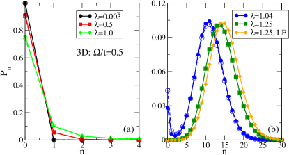
Figure 1: (color online) Phonon statistics for a 3D Holstein polaron with (a) small to intermediate, and (b) large effective couplings, and $\Omega/t=0.5$. MA⁽⁰⁾ (dashed lines, open symbols) and MA⁽¹⁾ (solid lines, solid symbols) results are shown. The Lang-Firsov (LF) asymptotic result is shown for $\lambda=1.25$.

GS phonon probabilities $P_{n}$ for a 3D Holstein polaron at several effective couplings $\lambda=g^{2}/(2dt\Omega)$ are shown in Fig. 1. 1D results are quite similar berciu:08 . At weak el-ph couplings, the polaron has few phonons in its cloud so $P_{n\geq 1}$ are small. At the crossover to a small polaron at $\lambda\sim 1$, the distribution changes abruptly and dramatically. As $\lambda\rightarrow\infty$, $P_{n}\rightarrow\frac{1}{n!}\left(\frac{g}{\Omega}\right)^{2n}e^{-{g^{2}\over\Omega^{2}}}$, the Lang-Firsov (LF) limit, already quite accurate for $\lambda=1.25$. The difference between MA⁽⁰⁾ and MA⁽¹⁾ is small. This is not surprising, since these probabilities are for the GS, which is already very accurately described by MA⁽⁰⁾ berciu:06 . The additional basis states added at the MA⁽¹⁾ level are essential to describe excited states in the polaron+one-phonon continuum, starting at $\Omega$ above the GS, and due to a phonon excited far from the polaron cloud berciu:06 . As we show now, they do have a significant effect on the $f_{n}(\omega)$ functions and therefore on the OC onset.

The $\omega$-dependence of the OC is dictated by $f_{n}(\omega)$. Eq. (6) shows that $f_{n}^{(0)}(\omega)$ becomes finite at $\omega+E_{0}-n\Omega\geq-2dt$, because the free-electron spectral weight is finite in $[-2dt,2dt]$. This implies that the onset of absorption is set by the $n=1$ curve to be $\omega_{\rm th}=-2dt-E_{0}+\Omega$, and larger $n$ contributions are shifted $(n-1)\Omega$ higher. As $\lambda$ increases and $E_{0}$ falls further below $-2dt$, this suggests that $\omega_{\rm th}$ increases monotonically. This is wrong: the OC onset is always expected at $\omega_{\rm th}=\Omega$ loos:07 ; mishchenko:03 . The discrepancy is easy to understand. The onset is due to absorption into the polaron+one-phonon continuum, which is not described by MA⁽⁰⁾, only by MA⁽¹⁾ and higher levels berciu:06 . Indeed, as shown in Fig. 2, there is a significant difference between the corresponding $n=1$ curves, and $f^{(1)}_{n=1}(\omega)$ does have an onset at $\omega_{\rm th}=\Omega$ even though it becomes hard to see at larger $\lambda$. The $n\geq 2$ curves are much less affected, in particular their onset roughly agrees with that predicted at MA⁽⁰⁾ level. Similar behavior is found in 1D, but the peak in each $f_{n}(\omega)$ moves towards the low-energy threshold goodvin:10 , as expected since the 1D free electron density of states is singular at the band-edge.

In Fig. 3, we plot the first, to our knowledge, complete set of OC curves reported for a 3D Holstein polaron, using both MA and DMC methods. On the whole, the agreement is excellent, especially between MA⁽¹⁾ and DMC. We find that MA⁽¹⁾ captures all the qualitative features of the full OC, as well as being able to resolve finer structure near the absorption onset. In particular, the “shoulder” that develops on the low-energy end of the OC spectrum could never be captured with perturbational methods. In the asymptotic $\lambda\rightarrow 0,\infty$ limits the curves are nearly indistinguishable, as expected since MA becomes exact in these limits. In the crossover regime $\lambda\sim 1$, the differences between MA⁽⁰⁾ and MA⁽¹⁾ are largest, as are those between MA and DMC results. Nevertheless, MA does a good job overall, especially considering that it is an efficient analytical approximation.

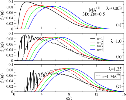
Figure 2: (color online) MA⁽¹⁾ functions $f^{(1)}_{n}(\omega)$, for (a) small, (b) medium, and (c) large el-ph coupling, at $\Omega/t=0.5,\eta=0.005$ in 3D. Also shown is $f^{(0)}_{n=1}(\omega)$ (dashed line).

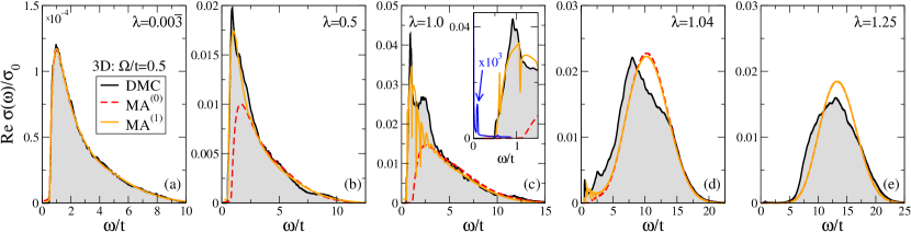
Figure 3: (color online) OC in units of $\sigma_{0}=\pi e^{2}t^{2}$ for a 3D Holstein polaron, calculated using MA⁽⁰⁾, MA⁽¹⁾ and DMC. The inset in panel (c) shows the absorption onset, and the no-vertex correction OC at $k_{B}T=0.01\Omega$, scaled by $10^{3}$ (thin blue line).

The shapes of the OC curves can now be understood using Eq. (2) and the data shown in Figs. 1 and 2. For small $\lambda$, $P_{n=1}$ is dominant and the OC is basically proportional to $f_{n=1}(\omega)$. Indeed, its rich structure is clearly visible in the OC, as is its threshold $\omega_{\rm th}=\Omega$. The $n\geq 2$ terms serve only to alter the high-energy tail. In the small polaron limit, however, $P_{n=1}\rightarrow 0$ and the OC is dominated by large $n$ contributions. Since these $f_{n}(\omega)$ curves have similar shapes and are shifted by $\Omega$ with respect to one other, the OC mirrors the LF Poissonian distribution of $P_{n}$. The peak location is also in good agreement with $2|E_{0}|=12\lambda t$, expected as $\lambda\rightarrow\infty$ Emin . This is because when the electron is moved to a neighboring site by optical absorption, it loses the polaronic binding energy $E_{0}$ and it also leaves behind excited phonons with the same energy. The structure of our expression (2) proves that not only the peak energy, but the very shape of the OC curve is determined by the probabilities $P_{n}^{(i)}$. In 1D (not shown), the $f_{n}(\omega)$ functions are more peaked and individual contributions can be seen in the OC, as $\Omega$-spaced kinks. The agreement with available 1D numerical data is of similar quality with that of Fig. 3 goodvin:10 .

Consider now the DMFT-like no-vertex correction approximation, in which the two-particle Green’s function in Eq. (3) is replaced by a convolution of polaron spectral weights (for details, see the supplementary material). The scaled result for $\lambda=1$, $k_{B}T=0.01\Omega$, is shown in Fig. 3(c). A prominent feature is the peak (marked by arrow) below $\omega_{\rm th}$, in agreement with low-$T$ data in Ref.  Fratini , where it was identified as an excitation from the GS into the first bound-state. Indeed, the peak is at $\sim 0.12t$, their energy difference. The peak likely vanishes at $T=0,\eta=0$, however this shows that a naive consideration of the convolution may lead to a qualitatively wrong idea of the OC structure. DMC and MA results do not show this peak, although the second bound state is visible in their spectral weight (see the supplementary material). Its absence implies a vanishing matrix element in Eq. (4), likely due to the different symmetry of the polaron wavefunction in the two states bayo . Clearly, Eq. (2) properly accounts for such selection rules. More analysis is provided in the supplementary material found at the end of this article.

$\lambda=$	$0.00\bar{3}$	$0.5$	$1.0$	$1.04$	$1.25$
MA(0)	0.0003	0.037	0.084	0.180	0.145
MA(1)	0.0003	0.048	0.107	0.180	0.145
DMC	0.0003	0.050	0.125	0.190	0.150

Table 1: Total integrated OC $S(\infty)/\sigma_{0}$ for the parameters used in Fig. 3, for MA⁽⁰⁾, MA⁽¹⁾, and DMC.

To further prove the accuracy of MA, we compare in Table 1 the total integrated OC, $S(\infty)=\int_{0}^{\infty}d\omega\,\sigma(\omega)$, for MA and DMC. The agreement is again very good, particularly at small and large $\lambda$, where we typically find less than $5\%$ difference. At intermediate couplings MA accounts for over $85\%$ of the total integrated OC, which is quite remarkable for an analytical approximation.

Knowledge of the total integrated OC can also be used to verify that MA satisfies the f-sum rule, given by maldague:77 :

$$-e^{2}aE_{\mathrm{kin}}=\frac{1}{\pi}{\cal D}+\frac{2}{\pi}S(\infty),$$ (7)

where $E_{\mathrm{kin}}$ is the GS polaron kinetic energy and ${\cal D}=\pi e^{2}a/m^{*}$ is the Drude weight kohn:64 , $m^{*}$ being the polaron effective mass. Both these quantities can be calculated from the GS properties of the polaron, using known MA methods berciu:06 . In all cases reported here, we have verified that the total integrated OC matches the expected value from the f-sum rule to at least three decimal places.

In conclusion, we have obtained the first accurate analytical non-perturbational expression for the $T=0$ optical conductivity of a Holstein polaron. It explains the shape of the OC curve by explicitly relating it to the statistics of the polaron cloud. We find no absorption below the threshold at $\Omega$ even if a second bound state exists, proving that Eq. (2) accounts for selection rules. Moreover, this work can be generalized for OC studies of polaronic systems with momentum-dependent el-ph coupling, and also disorder, in any dimension.

Acknowledgments: Work supported by NSERC and CIfAR (GLG and MB), and RFBR 10-02-00047a (ASM).

I Supplementary Material

I.1 Calculation of the matrix elements within MA⁽⁰⁾

First, we need to calculate the generalized single particle Green’s functions:

$$F_{nm}(\mathbf{q},\mathbf{Q},\omega)=\langle-{\mathbf{q}},n|c_{\mathbf{q}}\hat{G}(\omega)c_{\mathbf{Q}}^{\dagger}|-{\mathbf{Q}},m\rangle$$ (8)

where

$$|-\mathbf{q},n\rangle=\frac{1}{\sqrt{N}}\sum_{i}e^{-i\mathbf{q}\cdot\mathbf{R}_{i}}(b_{i}^{\dagger})^{n}|0\rangle$$ (9)

We use Dyson’s identity $\hat{G}(\omega)=\hat{G}_{0}(\omega)+\hat{G}(\omega)V\hat{G}_{0}(\omega)$ where $V$ is the el-ph interaction and $\hat{G}_{0}(\omega)$ is the resolvent for ${\cal H}_{0}={\cal H}-V$, plus the MA⁽⁰⁾ one-site cloud restriction, to find $F_{nm}(\mathbf{q},\mathbf{Q},\omega)=G_{0}(\mathbf{Q},\omega-m\Omega)[\delta_{\mathbf{q},\mathbf{Q}}\delta_{n,m}n!+mgf_{n,m-1}(\mathbf{q},\omega)+gf_{n,m+1}(\mathbf{q},\omega)]$. Here, the free propagator is $G_{0}(\mathbf{k},\omega)=(\omega+i\eta-\varepsilon_{\mathbf{k}})^{-1}$, and $f_{n,m}(\mathbf{q},\omega)=\frac{1}{N}\sum_{\mathbf{Q}}F_{nm}(\mathbf{q},\mathbf{Q},\omega)$ are partial momentum averages related to the ones calculated in Ref. berciu:06alt . They can therefore be calculated similarly; however, they depend on $\mathbf{q}$ only through $\varepsilon_{\mathbf{q}}$, therefore they are even functions whose contribution to $\sigma_{+}(\omega)$ vanishes after the sum over $\mathbf{q}$ because of the odd prefactor $\sin q$ coming from the current operator. As a result, within MA⁽⁰⁾ we can replace

$$F_{nm}(\mathbf{q},\mathbf{Q},\omega)\rightarrow G_{0}(\mathbf{Q},\omega-m\Omega)\delta_{\mathbf{q},\mathbf{Q}}\delta_{n,m}n!$$

in Eq. (5). The delta functions remove the sums over $m,\mathbf{Q}$. All that is left, then, is to find the residues $|\langle\psi_{0}|c_{\mathbf{q}}^{\dagger}|-{\mathbf{q}},n\rangle|^{2}$. To achieve this, consider the generalized single-electron Green’s functions:

$$F_{n}(\mathbf{q},\omega)=\langle 0|c_{\mathbf{k}=0}\hat{G}(\omega)c^{\dagger}_{\mathbf{q}}|-\mathbf{q},n\rangle.$$ (10)

These are also similar to the single particle Green’s functions calculated in Ref. berciu:06alt , and can be calculated in terms of continued fractions by the same means. Within MA⁽⁰⁾, they are equal to:

$$F_{n}(\mathbf{q},\omega)=\frac{G_{0}(\mathbf{q},\omega-n\Omega)}{\bar{g}_{0}(\omega-n\Omega)}A_{n,1}(\omega)G(\mathbf{k}=0,\omega).$$ (11)

where $G(\mathbf{k},\omega)=\langle 0|c_{\mathbf{k}}\hat{G}(\omega)c_{\mathbf{k}}^{\dagger}|0\rangle$ is the usual single-particle polaron Green’s function, and we define $A_{n,k}(\omega)=A_{n}(\omega)A_{n-1}(\omega)\cdots A_{k}(\omega)$ where the continuous fractions are berciu:06alt ; glen:07 :

$$A_{n}(\omega)=\frac{ng\bar{g}_{0}(\omega-n\Omega)}{1-g\bar{g}_{0}(\omega-n\Omega)A_{n+1}(\omega)}$$ (12)

and

$$\bar{g}_{0}(\omega)=\frac{1}{N}\sum_{\mathbf{q}}G_{0}(\mathbf{q},\omega)$$ (13)

is the momentum average of the bare propagator.

On the other hand, from its Lehmann representation:

$$F_{n}(\mathbf{q},\omega)=\sum_{\alpha}\frac{\langle 0|c_{\mathbf{k}=0}|\psi_{\alpha}\rangle\langle\psi_{\alpha}|c_{\mathbf{q}}^{\dagger}|-\mathbf{q},n\rangle}{\omega-E_{\alpha}+i\eta},$$ (14)

so its residue for $\omega=E_{0}$, the GS energy, is the product $\langle 0|c_{\mathbf{k}=0}|\psi_{\alpha}\rangle\langle\psi_{\alpha}|c_{\mathbf{q}}^{\dagger}|-\mathbf{q},n\rangle$. The first term is related to the GS quasiparticle weight $Z_{0}$, and the second is the overlap that we need. It follows that:

$$\langle\psi_{0}|c_{\mathbf{q}}^{\dagger}|-\mathbf{q},n\rangle=\frac{G_{0}(\mathbf{q},\omega-n\Omega)}{\bar{g}_{0}(\omega-n\Omega)}\sqrt{Z_{0}}A_{n,1}(E_{0}),$$ (15)

The $\omega$-independent part can be shown to be related to the probability to have $n$-particles at the electron site in the GS. In Ref. berciu:08alt , these probabilities were found to be:

$$P_{n}^{(0)}={Z_{0}\over n!}\left|A_{n,1}(E_{0})\right|^{2}$$ (16)

The $\omega$-dependent terms can be grouped together with the one from $F_{nm}(\mathbf{q},\mathbf{Q},\omega)$ into the corresponding function $f_{n}^{(0)}(\omega)$, whose expression is given in Eq. (6).

The MA⁽¹⁾ calculations proceed along similar lines, but are much more involved because of the enlarged basis. The full details will be presented in a longer publication.

I.2 The approximation of no current vertex corrections

The essence of this approximation is to replace the two-particle Green’s functions appearing in $\sigma^{+}(\omega)$, namely $\langle\psi_{0}|c^{\dagger}_{\mathbf{Q}}c_{\mathbf{Q}}\hat{G}(\omega)c^{\dagger}_{\mathbf{q}}c_{\mathbf{q}}|\psi_{0}\rangle$, by a convolution of the single-particle spectral weights. The procedure is reviewed in detail in Ref. loos . The regular part of the conductivity, at finite $T$ and on a cubic lattice, is then found to be [their Eq. (19)]:

$$\sigma(\omega)={4\sigma_{0}\over\omega N}\sum_{\mathbf{k}}\sin^{2}k\int_{-\infty}^{\infty}d\omega^{\prime}A(\mathbf{k},\omega^{\prime})A(\mathbf{k},\omega+\omega^{\prime})\\ \times\left[f(\omega^{\prime})-f(\omega+\omega^{\prime})\right].$$ (17)

Here $A(\mathbf{k},\omega)$ is the polaron spectral weight and $f(\epsilon)=(e^{\beta\epsilon}+1)^{-1}$ is the Dirac function. This is the same formula used in DMFT, see for example Eq. (3) in Ref. Fratini1 . The difference is that in DMFT, the integral over the Brillouin zone is replaced by an integral over energies $\epsilon=\epsilon_{\mathbf{k}}$ (they also replace $\omega^{\prime}\rightarrow\nu$). This explains the appearance of the density of states $N_{\epsilon}$ of the free lattice, and of the DMFT vertex $\Phi_{\epsilon}$ which is the equivalent of the $\sin^{2}k$ in the above equation. Of course, within DMFT one uses the DMFT self-energy in the spectral weight.

In order to limit the quantitative differences of the DOS used in DMFT, which is for a Bethe lattice, whereas our other results are for a cubic lattice, we use Eq. (17) for a cubic lattice to test this approximation. Also, for convenience, we use the MA self-energy in the spectral weight. This is simpler because in order to calculate the DMFT self-energy, one needs to go through iterations to reach self-consistency. In any event, the MA and DMFT self-energies are qualitatively and even quantitatively in fairly good agreement, as shown in the Appendix of Ref. berciu:06alt . Moreover, it has been shown that the MA spectral weights are very accurate, satisfying eight sum rules exactly (within MA⁽¹⁾), therefore using the MA self-energy and its corresponding spectral weight can lead, at most, to modest quantitative differences.

Since the MA⁽¹⁾ self-energy is momentum-independent (momentum dependence appears only from the MA⁽²⁾ level), we can carry the integral over the Brillouin zone as follows. We rewrite the spectral weights as

$$A(\mathbf{k},\omega)=-{1\over\pi}G(\mathbf{k},\omega)={i\over 2\pi}\left[{1\over\omega+i\eta-\epsilon_{\mathbf{k}}-\Sigma(\omega)}-{1\over\omega-i\eta-\epsilon_{\mathbf{k}}-\Sigma^{*}(\omega)}\right]$$

The product of two spectral weights will result in a sum of 4 terms that can be further factorized, for example:

$${1\over\omega^{\prime}+i\eta-\epsilon_{\mathbf{k}}-\Sigma(\omega^{\prime})}\cdot{1\over\omega+\omega^{\prime}+i\eta-\epsilon_{\mathbf{k}}-\Sigma(\omega+\omega^{\prime})}\\ ={1\over\omega-\Sigma(\omega+\omega^{\prime})+\Sigma(\omega^{\prime})}\left[{1\over\omega^{\prime}+i\eta-\epsilon_{\mathbf{k}}-\Sigma(\omega^{\prime})}-{1\over\omega+\omega^{\prime}+i\eta-\epsilon_{\mathbf{k}}-\Sigma(\omega+\omega^{\prime})}\right\}$$ (18)

As a result, the integral over the Brillouin zone now becomes a simple momentum average of the bare propagator (with shifted frequency) times the $\sin^{2}{k_{x}}$ term. One integral can be done analytically, and the other two numerically like other similar momentum averages calculated for MA⁽²⁾, see Ref. berciu:06alt . One is then left with evaluating the integral over $\omega^{\prime}$ numerically as well.

One can approach the $T=0$ limit either directly by replacing the Fermi-Dirac distribution with a Heaviside function, as done in Ref. loos ; or by calculating the $T\rightarrow 0$ limit of the ratio detailed in Refs. Fratini1 ; Fratini2 . Either approach has its own numerical challenges, and overall we find both procedures to be more time consuming than evaluating our OC formula, even when the computationally trivial MA self-energy is used in the spectral weight. Note, also, that our OC formula is formulated directly for $T=0$ and therefore one needs not worry about how to properly approach this limit.

The $\mathbf{k}=0$ spectral weight for the polaron, at intermediary coupling $\lambda=1$, is shown in Fig. 4. The GS peak still has considerable weight $Z_{0}\sim 0.5$, and just above it we see the peak corresponding to the second bound state, followed by the continuum and higher energy features. The rough expectation is that a convolution of this curve with itself will show a first peak when the two curves are shifted by $E_{1}-E_{0}$, the energy difference between the two bound states; also, absorption into the continuum will appear for frequencies $\omega>\Omega$.

Figure 4: Spectral weight $A(\mathbf{k}=0,\omega)$ for the 3D Holstein polaron, for $\lambda=1,\Omega=0.5t,\eta=10^{-3}$. The GS energy is $E_{0}=-6.65t$, and the first bound state is at $E_{1}=-6.53t$. The continuum onset is visible at $E_{0}+\Omega$.

Thus, the naive expectation based on the convolution is that as soon as the second bound state is formed, there should be absorption into it, at energies below the threshold $\Omega$. This is also what is shown by the full DMFT calculations at very low temperatures, see curve of Fig. 2 and its interpretation from Fig. 3 in Ref. Fratini1 , in qualitative agreement with our own calculation for $k_{B}T=0.01\Omega$, shown in Fig. 3(c) of the main article.

In reality, very careful analysis suggests that the weight of this peak decreases monotonically with $T$, and therefore at $T=0$ it is very likely that this approach also predicts no absorption below the threshold at $\Omega$, in agreement with the DMC and MA approaches. Our understanding of the disappearance of this peak is that it comes from the fact that the $k=0$ convolution is multiplied by $\sin^{2}k$, so strictly speaking there is no contribution to the OC from the GS momentum, unless some “thermal broadening” is allowed at non-zero temperatures.

Since the exact DMC calculation finds no such absorption into the second bound state at any $\lambda$, the matrix element for this transition must be zero, likely because of the different symmetry of the phonon clouds in the two states, as discussed in detail for 1D systems in Ref. new . Clearly, our MA-based OC formula captures this selection rule properly – note that the generalized single-particle Green’s functions that appear in it are different from the Green’s function that gives the spectral weight.

On the other hand, there is nothing in the spectral weight that encodes the symmetry of the wavefunction associated with a bound state, for example one cannot distinguish the parity of a state by looking at the plot of the spectral weight. Thus, it seems to us that generically, one should expect the convolution approximation to fail to properly account for selection rules.

In fact, this statement can be tested in 1D, where as shown in Ref. new , one may expect higher energy bound states, some of which are optically active. In other models, it has been suggested that there may even be bound-states below the continuum which are not visible in the spectral weight, because their quasiparticle weight vanishes for symmetry reasons bayoalt – if such states are optically active, absorption associated with them would certainly not be predicted by the convolution approximation. Such a study will be undertaken elsewhere, and should clarify whether the agreement in 3D regarding the lack of sub-threshold absorption in the no-current vertex approximation is accidental, or it actually has a more robust explanation. In any event, this is probably somewhat of an academic discussion, since such multiple bound states appear only at large effective couplings $\lambda$ where the bulk of the optical absorption is at very much higher energies, and in measurements the very small signal at the threshold may be buried in noise.

Be that as it may, to us it appears that besides being numerically more difficult to evaluate and less tested in terms of its accuracy for sum rules etc, the no-current vertex approximation also fails to provide the insight into the overall evolution of the OC curves that is afforded by our new formula. Moreover, MA has already been demonstrated to generalize very successfully to models where the coupling depends on the phonon and electron momentum, and we expect similar success in modeling their OC. Such models have strongly momentum-dependent self-energies, and are unlikely to be described accurately with a local-approximation like DMFT.

References

- (1) L. D. Landau, Phys. Z. Sowjet 3, 644 (1933).
- (2) P. Calvani et al., J. Supercond. 10, 293 (1997).
- (3) O. Gunnarsson and O. Rösch, J. Phys.: Condens. Matter 20, 043201 (2008).
- (4) Ch. Hartinger et al., Phys. Rev. B, 73, 024408 (2006).
- (5) S. El Shawish et al., Phys. Rev. B 67, 014301 (203); J. Loos et al., J. Phys.: Cond. Matt. 19, 236233 (2007); A. Alvermann et al., Phys. Rev. B 81, 165113 (2010); G. De Filippis et al., Phys. Rev. B 72, 014307 (2005).
- (6) H. Fehske et al., Z. Phys. B 104, 619 (1997).
- (7) A. S. Mishchenko et al., Phys. Rev. Lett. 91, 236401 (2003); G. De Filippis et al., Phys. Rev. Lett. 96, 136405 (2006); A. S. Mishchenko et al., Phys. Rev. Lett. 100, 166401 (2008).
- (8) for example, see D. Emin, Adv. Phys. 24, 305 (1975).
- (9) S. Fratini, F. de Pasquale, and S. Ciuchi, Phys. Rev. B 63, 153101 (2001); S. Fratini and S. Ciuchi, Phys. Rev. B 74, 075101 (2006).
- (10) M. Berciu and G. L. Goodvin, Phys. Rev. B 76, 165109 (2007); M. Berciu, Phys. Rev. Lett. 98, 209702 (2007).
- (11) G. L. Goodvin and M. Berciu, Phys. Rev. B 78, 235120 (2008); M. Berciu and H. Fehske, Phys. Rev. B 82, 085116 (2010); D. Marchand et al., Phys. Rev. Lett. 105, 266605 (2010).
- (12) M. Berciu, A.S. Mishchenko, and N. Nagaosa, EuroPhys. Lett. 89, 37007 (2010); G. L. Goodvin, L. Covaci, and M. Berciu, Phys. Rev. Lett. 103, 176402 (2009).
- (13) T. Holstein, Ann. Phys. (N.Y.) 8, 325 (1959).
- (14) G. D. Mahan, Many particle physics (Plenum, NY, 1981).
- (15) H. Fehske et al., Phys. Rev. B 61, 8016 (2000).
- (16) O. S. Barisic, Phys. Rev. Lett. 98, 209701 (2007).
- (17) M. Berciu, Can. J. Phys. 86, 523 (2007).
- (18) G. L. Goodvin and M. Berciu, unpublished.
- (19) O. S. Barisic, Phys. Rev. B 69, 064302 (2004); B. Lau, M. Berciu and G.A. Sawatzky, Phys. Rev. B 76, 174305 (2007).
- (20) P. F. Maldague, Phys. Rev. B 16, 2437 (1977).
- (21) W. Kohn, Phys. Rev. 133, A171 (1964).

References

- (1) M. Berciu and G. L. Goodvin, Phys. Rev. B 76, 165109 (2007).
- (2) M. Berciu, Phys. Rev. Lett. 97, 036402 (2006); G.L. Goodvin, M. Berciu, and G.A. Sawatzky, Phys. Rev. B 74, 245104 (2006).
- (3) M. Berciu, Can. J. Phys. 86, 523 (2007).
- (4) J. Loos, M. Hohenadler, A. Alvermann, H. Fehske, J. Phys.: Cond. Matt. 19, 236233 (2007).
- (5) S. Fratini, F. de Pasquale, and S. Ciuchi, Phys. Rev. B 63, 153101 (2001).
- (6) S. Fratini and S. Ciuchi, Phys. Rev. B 74, 075101 (2006).
- (7) O. S. Barisic, Phys. Rev. B 69, 064302 (2004).
- (8) B. Lau, M. Berciu and G.A. Sawatzky, Phys. Rev. B 76, 174305 (2007).