Trispectrum estimation in various models of equilateral type non-Gaussianity

Abstract

We calculate the shape correlations between trispectra in various equilateral non-Gaussian models, including DBI inflation, ghost inflation and Lifshitz scalars, using the full trispectrum as well as the reduced trispectum. We find that most theoretical models are distinguishable from the shapes of primordial trispectra except for several exceptions where it is difficult to discriminate between the models, such as single field DBI inflation and a Lifshitz scalar model. We introduce an estimator for the amplitude of the trispectrum, $g_{\rm NL}^{equil}$ and relate it to model parameters in various models. Using constraints on $g_{\rm NL}^{equil}$ from WMAP5, we give constraints on the model parameters.

I Introduction

Almost scale-invariant and Gaussian primordial cosmological perturbations predicted by inflation are consistent with observational data. While this suggests that inflation did happen in the early universe, there still remain many important questions about inflation. One of the most important problems is to distinguish between various inflationary models as there are still many models that are consistent with observational data at present. For this purpose, it is necessary to have further information about the early universe such as deviations from Gaussianity (non-Gaussianity) of the primordial perturbations and primordial gravitational waves. In this paper, we focus on primordial non-Gaussianity.

Actually, the statistical properties of primordial fluctuations provide crucial information on the physics of the very early universe Komatsu:2010fb ; Smith:2009jr ; Senatore:2009gt ; Fergusson:2010dm (see Bartolo:2004if for a review). In the simplest single field inflation models where the scalar field has a canonical kinetic term and quantum fluctuations are generated from the standard Bunch-Davis vacuum, non-Gaussianity of the fluctuations is too small to be observed even with future experiments Acquaviva:2002ud ; Maldacena:2002vr ; Seery:2005wm . Thus, the detection of non-negligible deviations from Gaussianity of primordial fluctuations will have a huge impact on the models of the early universe. So far, most of the studies have focused on the leading order non-Gaussianity measured by the three-point function of Cosmic Microwave Background (CMB) anisotropies, i.e. the bispectrum Verde:1999ij ; Wang:1999vf ; Komatsu:2001rj . Especially, the optimal method of extracting the bispectrum from the CMB data has been sufficiently developed Komatsu:2003iq ; Babich:2004gb ; Babich:2005en ; Creminelli:2005hu ; Creminelli:2006gc ; Yadav:2007rk ; Yadav:2007ny (for a more general approach, see Fergusson:2006pr ; Fergusson:2008ra ; Fergusson:2009nv ). However, the bispectrum includes only a part of information about non-Gaussianity and many models can predict similar bispectra.

For example, k-inflation ArmendarizPicon:1999rj ; Garriga:1999vw and Dirac-Born-Infeld (DBI) inflation Silverstein:2003hf are shown to predict almost equilateral type bispectrum (see Koyama:2010xj ; Chen:2010xka for reviews). However, future experiments like Planck Planck can also prove the higher order statistics such as the trispectrum Hu:2001fa ; Okamoto:2002ik ; Kogo:2006kh which gives information that cannot be obtained from the bispectrum Seery:2006js ; Seery:2006vu ; Byrnes:2006vq .

Non-Gaussianity of the observed CMB anisotropies comes from not only the primordial origin but also the non-linear effects in the CMB at late times such as the coupling between Integrated Sachs-Wolfe (ISW) effect and the weak gravitational lensing arXiv:1003.6097 . However, these non-linear effects can be negligible compared with the primordial non-Gaussainity in the models such as DBI inflation and ghost inflation where large primordial non-Gaussianity is predicted and it is the dominant contribution to the observed non-Gaussianity. In this paper, we focus on large primordial non-Gaussianity.

While the trispectrum has more information, it requires more work to understand how to distinguish between various trispectra predicted in many theoretical models and how to measure the amplitude of the trispectrum because it has more parameters than the bispectrum. To estimate an overlap between the shapes of two different trispectra, the shape correlator was introduced by Regan et.al Regan et al. (2010) based on the reduced trispectrum. Furthermore, based on this shape correlator, two of us investigated an estimator $g_{\rm NL}^{equil}$ to measure the amplitude of the trispectrum in some equilateral type non-Gaussian models, like k-inflation, single field DBI inflation and multi-field DBI inflation Mizuno:2010by .

Recently, the shape dependence of the trispectra from ghost inflation model ArkaniHamed:2003uy ; ArkaniHamed:2003uz and Lifshitz scalar model have been calculated in Refs. Izumi:2010wm ; Huang:2010ab and Ref. Izumi:2010yn . These models are known to give equilateral type bispectra. For Lifshitz scalar model, we will see that there is no natural way to decompose the full trispectrum into the reduced trispectra in some cases and the shape correlator based on the reduced trispectrum is not necessarily well-defined. Therefore, in this paper, we consider an implementation of the shape correlator of the primordial trispectrum using the full trispectrum so that we can calculate the shape correlations and investigate estimators in equilateral type non-Gaussian models including ghost inflation and Lifshitz scalar.

The rest of this paper is organised as follows. In section II, we introduce two shape correlators defined in different ways where one is defined based on the reduced trispectrum and the other is based on the full trispectrum. In section III, we calculate the shape correlations of the trispectra among various theoretical models; DBI inflation, ghost inflation and Lifshitz scalar. In section IV, we express the estimators $g_{\rm NL}^{equil}$ in terms of the model parameters, which is useful to constrain the model parameters from future experiments. We also give constraints on model parameters using WMAP constraints on $g_{\rm NL}^{equil}$ obtained in Fergusson:2010gn . Section V is devoted to the summary and discussions of this paper. In appendix sections A, B and C, we review the shape functions of the reduced trispectra in DBI inflation model, ghost inflation model and Lifshitz scalar model.

II Two types of shape correlators

In this section, we introduce two shape correlators. One is introduced by Regan Regan et al. (2010) and we review this method in section II.1. In this method, the shape correlators are defined based on the reduced trispectrum. Although the reduced trispectum includes all information of the original trispectrum, there is no unique way to decompose the total trispectrum into the reduced trispectrum. Then there appears an ambiguity in the definition of shape correlator based on the reduced trispectrum; a different choice of the reduced trispectrum gives a different shape correlator.

Before discussing the shape correlators, we review the definition of the trispectrum. The trispectrum $T_{\zeta}({\bf k}_{1},{\bf k}_{2},{\bf k}_{3},{\bf k}_{4})$ of the curvature perturbation $\zeta$ is defined as

$$\langle\zeta({\bf k}_{1})\zeta({\bf k}_{2})\zeta({\bf k}_{3})\zeta({\bf k}_{4})\rangle_{c}=(2\pi)^{3}\delta^{3}({\bf k}_{1}+{\bf k}_{2}+{\bf k}_{3}+{\bf k}_{4})T_{\zeta}({\bf k}_{1},{\bf k}_{2},{\bf k}_{3},{\bf k}_{4}),$$ (1)

where $\zeta({\bf k}_{1})$ is a Fourier component with the momentum ${\bf k}_{1}$ and the subscript “$c$” in the left hand side denotes the connected component. The trispectrum $T_{\zeta}({\bf k}_{1},{\bf k}_{2},{\bf k}_{3},{\bf k}_{4})$ generally depends on four three-momenta, namely twelve parameters. Assuming isotropy and homogeneity of the universe on large scales, the number of parameters reduces to six.

II.1 The shape correlator based on the reduced trispectrum

Here, we review the shape correlator discussed in Regan et al. (2010). First we exploit the symmetry of the trispectrum to define the reduced trispectrum as follows Hu:2001fa . We rewrite the definition of the trispectrum as

$$\langle\zeta({\bf k_{1}})\zeta({\bf k_{2}})\zeta({\bf k_{3}})\zeta({\bf k_{4}})\rangle_{c} = (2\pi)^{3}\int d^{3}K\bigl{[}\delta({\bf k_{1}}+{\bf k_{2}}-{\bf K})\delta({\bf k_{3}}+{\bf k_{4}}+{\bf K})\mathcal{T}_{\zeta}({\bf k_{1}},{\bf k_{2}},{\bf k_{3}},{\bf k_{4}};{\bf K})$$ (2)

$$+({\bf k_{2}}\leftrightarrow{\bf k_{3}})+({\bf k_{2}}\leftrightarrow{\bf k_{4}})\bigr{]}\,.$$

Because of the symmetry of the trispectrum, the reduced trispectrum includes all information of the original trispectrum Hu:2001fa . However, this decomposition of the trispectrum is not unique because there is an ambiguity in choosing K in Eq. (2). In some cases, there is a natural choice of the reduced trispectrum. For example, in the case of trispectrum produced by two three-point vertices, it consists of s-, t- and u-channels. Then we can decompose the trispectrum into three parts accordingly and define the reduced trispectrum in a natural way.

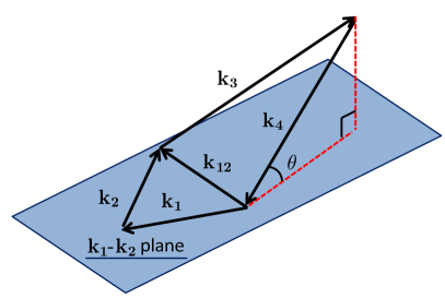
Figure 1: definition of $\theta_{4}$

The reduced trispectrum $\mathcal{T}_{\zeta}({\bf k_{1}},{\bf k_{2}},{\bf k_{3}},{\bf k_{4}};{\bf K})$ depends on six variables and we can choose them to be $(k_{1},k_{2},k_{3},k_{4},k_{12},\theta_{4})$ where $\theta_{4}$ represents the deviation of the quadrilateral from planarity which is specified by the triangle $(k_{1},k_{2},k_{12})$ (see Fig 1). From the geometric restriction, the range of $\theta_{4}$ is constrained as

$$\frac{|k_{4}^{2}+k_{12}^{2}-k_{3}^{2}|}{2k_{12}k_{4}}\leq\cos\theta_{4}\leq 1.$$ (3)

Motivated by the relation between the CMB trispectrum and the trispectrum for $\zeta$, we define the shape function for the reduced trispectrum as

$$S_{\mathcal{T}}(k_{1},k_{2},k_{3},k_{4},k_{12},\theta_{4})=(k_{1}k_{2}k_{3}k_{4})^{2}k_{12}\mathcal{T}_{\zeta}(k_{1},k_{2},k_{3},k_{4};k_{12},\theta_{4})\,.$$ (4)

Regan et al. Regan et al. (2010) proposed to define an inner product between two different shape functions $S_{\mathcal{T}}$ and $S_{\mathcal{T}^{\prime}}$ as

$$F(S_{\mathcal{T}},S_{\mathcal{T}^{\prime}})$$

$$\qquad=\int dk_{1}dk_{2}dk_{3}dk_{4}dk_{12}\int d(\cos\theta_{4})S_{\mathcal{T}}(k_{1},k_{2},k_{3},k_{4},k_{12},\theta_{4})S_{\mathcal{T}^{\prime}}(k_{1},k_{2},k_{3},k_{4},k_{12},\theta_{4})w(k_{1},k_{2},k_{3},k_{4},k_{12})\,,$$ (5)

where $w$ is an appropriate weight function. The weight function should be chosen such that $S^{2}w$ in $k$ space produces the same scaling as the estimator in $l$ space and we adopt the one used in Ref. Regan et al. (2010) ,

$$w(k_{1},k_{2},k_{3},k_{4},k_{12})=\frac{k_{12}}{(k_{1}+k_{2}+k_{12})^{2}(k_{3}+k_{4}+k_{12})^{2}}\,.$$ (6)

The integration range of the momenta $k_{1}$, $k_{2}$, $k_{3},$ $k_{4}$, $k_{12}$ in the integral of Eq. (5) is determined by the triangle inequality of the momenta. Namely, the conditions to satisfy ${\bf k_{12}}={\bf k_{1}}+{\bf k_{2}}$ are

$$k_{12}\leq k_{1}+k_{2},\qquad k_{1}\leq k_{12}+k_{2}\qquad\mbox{and}\qquad k_{2}\leq k_{12}+k_{1}.$$ (7)

Moreover, from the momentum conservation we obtain $-{\bf k_{12}}={\bf k_{3}}+{\bf k_{4}}$, and thus the conditions

$$k_{12}\leq k_{3}+k_{4},\qquad k_{3}\leq k_{12}+k_{4}\qquad\mbox{and}\qquad k_{4}\leq k_{12}+k_{3},$$ (8)

must be also imposed. The integration range of $\cos\theta_{4}$ is fixed by inequality (3). Due to the symmetry under interchange of $k_{1}$ and $k_{2}$, we can confine the integration range to $k_{1}\geq k_{2}$. With this choice of weight, the shape correlator is defined as

$$\bar{\mathcal{C}}(S_{\mathcal{T}},S_{\mathcal{T}^{\prime}})=\frac{F(S_{\mathcal{T}},S_{\mathcal{T}^{\prime}})}{\sqrt{F(S_{\mathcal{T}},S_{\mathcal{T}})F(S_{\mathcal{T}^{\prime}},S_{\mathcal{T}^{\prime}})}}\,.$$ (9)

II.2 The shape correlator based on the full trispectrum

In this subsection, we implement the shape correlator using the full trispectrum $T_{\zeta}$. As we mentioned in the previous subsection, while the reduced trispectrum has all information of the original trispectrum, the decomposition of the full trispectrum into the reduced trispectra is not unique. If all momenta appear symmetrically in the definition of the correlator, the obtained correlation is independent of the choice of the reduced trispectrum. However, the definition given by Eq. (5) apparently breaks the symmetry because of the integration variables $k_{12}$ and $\theta_{4}$. Therefore, in order to define the correlator uniquely, we must use the full trispectrum in the definition of the shape correlator.

The shape correlator based on the full trispectrum is defined in a similar way with the one based on the reduced trispectrum. Namely, we begin with defining the shape function as

$$S_{T}(k_{1},k_{2},k_{3},k_{4},k_{12},\theta_{4})=(k_{1}k_{2}k_{3}k_{4})^{2}k_{12}T_{\zeta}(k_{1},k_{2},k_{3},k_{4};k_{12},\theta_{4})\,.$$ (10)

The inner product is defined as

$$F(S_{T},S_{T^{\prime}})$$

$$\quad=\int dk_{1}dk_{2}dk_{3}dk_{4}dk_{12}\int d(\cos\theta_{4})S_{T}(k_{1},k_{2},k_{3},k_{4},k_{12},\theta_{4})S_{T^{\prime}}(k_{1},k_{2},k_{3},k_{4},k_{12},\theta_{4})w(k_{1},k_{2},k_{3},k_{4},k_{12})\,.$$ (11)

where we use the same weight function $w$ as that in the case of reduced trispectrum. The domain of integration in Eq. (11) is basically the same as that for the reduced trispectrum, i.e. inequalities (3), (7) and (8). However, since the symmetry under interchange of $k_{1}$ and $k_{2}$ still remains, the additional condition $k_{1}\geq k_{2}$ does not change the final value of the shape correlator.Therefore, we adopt inequalities (3), (7), (8) and $k_{1}\geq k_{2}$ as the domain of integration.

The shape correlator is defined in the same way

$$\bar{\mathcal{C}}(S_{T},S_{T^{\prime}})=\frac{F(S_{T},S_{T^{\prime}})}{\sqrt{F(S_{T},S_{T})F(S_{T^{\prime}},S_{T^{\prime}})}}\,.$$ (12)

III Shape correlations

In this section, we explicitly calculate the shape correlations among trispectra predicted by various theoretical models. The main purpose of investing the trispectrum is discriminating between models which are hard to be distinguished by the bispectrum. Thus we concentrate on the shape correlations among the models where the bispectrum is dominated by the equilateral type one; single field and multi-field DBI inflation models, ghost inflation model and Lifshitz scalar model.

The explicit forms of the shape functions are calculated in Appendixes. $S_{\mathcal{T}}^{DBI(\sigma)}$, $S_{\mathcal{T}}^{DBI(s)}$ and $S_{\mathcal{T}}^{ghost}$ are defined as the shape functions in single field DBI Inflation, multi-field DBI inflation and ghost inflation, respectively. Explicit forms of them are written in Eqs.(57), (60) and (63). In Lifshitz scalar field, there are a few contributions of Trispectrum and it depends on the parameters in the theory. We define $S_{\mathcal{T}}^{h(se,11)}$, $S_{\mathcal{T}}^{h(se,12)}$, $S_{\mathcal{T}}^{h(se,13)}$, $S_{\mathcal{T}}^{h(ci,1)}$, $S_{\mathcal{T}}^{h(ci,2)}$, and $S_{\mathcal{T}}^{h(ci,3)}$ as the shape functions of respective contributions. We show explicit forms of them in Eqs.(65) and (66).

Furthermore, the shape given by $S^{c1}_{\mathcal{T}}$ (see Eq. (35)) can be written in a separable form Chen:2009bc and it provides a fast estimator for the equilateral type trispectrum Regan et al. (2010); Mizuno:2010by . This means that if the shape function for the trispectrum is highly correlated with $S^{c1}_{\mathcal{T}}$, we can constrain the model parameters from the amplitude of the trispectrum in a very simple and fast way as we will discuss in Sec. IV. Therefore, we also calculate the shape correlations of the trispectra predicted by theories mentioned above with $S^{c1}_{\mathcal{T}}$.

Another motivation for calculating the shape correlations is to check the difference between the two shape correlators that we introduced in the previous section. As we mentioned in the previous section, the shape correlation based on the reduced trispectrum depends on the way to decompose the full trispectrum into the reduced trispectra. Thus strictly speaking, we should use the full tripsectrum when calculating the shape correlation. However, the calculation is easier for the shape correlation using the reduced trispectrum. If the difference is insignificant, we may still use the reduced trispectrum to calculate the shape correlator.

III.1 Shape correlations based on the reduced trispectrum

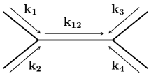
Figure 2: scalar exchange diagram with $k_{12}$ inner propagator

Here, we calculate the shape correlations among the theoretical models based on the reduced trispectrum. We must specify how we decompose the full trispectrum into reduced trispectra. One natural way is to decompose it so that one of the reduced trispectrum depends only on five parameters $k_{1}$, $k_{2}$, $k_{3}$, $k_{4}$ and $k_{12}$. Except for the case of the trispectrum obtained by the contact interaction in Lifshitz scalar model for $i=3$ in Eq. (66), it is possible to find such a decomposition. In fact, in the case of the scalar exchange trispectrum, this is always the case. The contribution of the trispectrum from the scalar exchange can be decomposed into s-, t- and u-channels and one of the channel depends only on five parameters $k_{1}$, $k_{2}$, $k_{3}$, $k_{4}$ and $k_{12}$. This can be understood as follows. The diagram of the scalar exchange trispectrum has one inner propagator. In the diagram where the momentum of the inner propagator is $k_{12}$, the propagators with momenta $k_{1}$ and $k_{2}$ meet directly at one vertex. On the other hand, the propagators with momenta $k_{3}$ and $k_{4}$ meet at the other vertex (see Fig. 2). Then, the trispectrum from Fig. 2 is written in terms of $k_{1}$, $k_{2}$, $k_{3}$, $k_{4}$, $k_{12}$, $\bf k_{1}\cdot k_{2}$ and $\bf k_{3}\cdot k_{4}$. The inner products $\bf k_{1}\cdot k_{2}$ and $\bf k_{3}\cdot k_{4}$ can be expressed as $(k_{12}^{2}-k_{1}^{2}-k_{2}^{2})/2$ and $(k_{12}^{2}-k_{3}^{2}-k_{4}^{2})/2$, respectively. Therefore, the trispectrum from Fig. 2 depends only on $k_{1}$, $k_{2}$, $k_{3}$, $k_{4}$ and $k_{12}$. Moreover, in most models even the contact interaction trispectrum can be also decomposed in such a way that the reduced trispectrum only depends on $k_{1}$, $k_{2}$, $k_{3}$, $k_{4}$ and $k_{12}$. In the contact interaction, there are no inner propagators. Thus the dependence on $k_{12}$, $k_{13}$ and $k_{14}$ stem only from the derivative coupling such as $(\vec{\nabla}_{i}\phi)^{2}\phi^{2}$. Only when the product of $k_{12}$ and $k_{13}$ appear in a contact interaction trispectrum, the trispectrum can not be decomposed in the way so that reduced trispectrum depends only on $k_{1}$, $k_{2}$, $k_{3}$, $k_{4}$ and $k_{12}$. This actually happens for the contact interaction in Lifshitz scalar field for $i=3$ in Eq. (66).

In appendix A, B, C, we summarise the explicit expressions of the shape functions defined by the reduced trispectra in single field and multi-field DBI inflation models, ghost inflation model and Lifshitz scalar model, respectively. As is mentioned above, except for the one corresponding to the contact interaction in Lifshitz scalar field for $i=3$ in (66), they depend only on five parameters $k_{1}$, $k_{2}$, $k_{3}$, $k_{4}$ and $k_{12}$. For the trispectrum coming from the contact interaction in Lifshitz scalar field for $i=3$ in Eq. (66), we need to define the reduced trispectrum so that it is symmetric under the transpose among $\boldsymbol{k_{1}}$, $\boldsymbol{k_{2}}$, $\boldsymbol{k_{3}}$ and $\boldsymbol{k_{4}}$.

The shape correlations among the models are summarised in Table 1. From this table, $S^{DBI(\sigma)}_{\mathcal{T}}$ and $S^{h(se,22)}_{\mathcal{T}}$ turn out to be highly correlated with $S^{c1}_{\mathcal{T}}$.

III.2 Shape correlations based on the full trispectrum

Now, we move to the shape correlations based on the full trispectrum. With Eqs. (1) and (2), the full trispectrum is obtained from the reduced trispectrum summarised in the appendix sections, by adding their permutations $(k_{2}\leftrightarrow k_{3})$ and $(k_{2}\leftrightarrow k_{4})$. Then, the shape functions based on the full trispectrum can be written by $k_{1}$, $k_{2}$, $k_{3}$, $k_{4}$, $k_{12}$, $k_{13}$ and $k_{14}$. We substitute the shape functions of the full trispectra into the definition of the shape correlator (12). Thus, we need to express $k_{13}$ and $k_{14}$ in terms of $k_{1}$, $k_{2}$, $k_{3}$, $k_{4}$, $k_{12}$ and $\theta_{4}$. We find that these variables are expressed as

$$k_{13} = \biggl{\{}(k_{2}^{2}+k_{4}^{2}-\frac{1}{2k_{12}^{2}}(k_{2}^{2}+k_{12}^{2}-k_{1}^{2})(k_{4}^{2}+k_{12}^{2}-k_{3}^{2})$$

$$\mp\frac{1}{2k_{12}^{2}}\sqrt{4k_{2}^{2}k_{12}^{2}-(k_{2}^{2}+k_{12}^{2}-k_{1}^{2})^{2}}\sqrt{4k_{4}^{2}k_{12}^{2}\cos^{2}\theta_{4}-(k_{4}^{2}+k_{12}^{2}-k_{3}^{2})^{2}})\biggr{\}}^{1/2}\,,$$

$$k_{14} = \biggl{\{}(k_{1}^{2}+k_{4}^{2}-\frac{1}{2k_{12}^{2}}(k_{1}^{2}+k_{12}^{2}-k_{2}^{2})(k_{4}^{2}+k_{12}^{2}-k_{3}^{2})$$ (13)

$$\mp\frac{1}{2k_{12}^{2}}\sqrt{4k_{1}^{2}k_{12}^{2}-(k_{1}^{2}+k_{12}^{2}-k_{2}^{2})^{2}}\sqrt{4k_{4}^{2}k_{12}^{2}\cos^{2}\theta_{4}-(k_{4}^{2}+k_{12}^{2}-k_{3}^{2})^{2}})\biggr{\}}^{1/2}\,,$$

where $\pm$ is determined by the configurations of the momenta; if the angle between the planes which are specified by $(k_{1},k_{2},k_{12})$-triangle and $(k_{3},k_{4},k_{12})$-triangle, $\alpha$, is smaller than the right angle (see Fig. 3), the corresponding sign is the minus ($-$). Otherwise, we should choose the plus ($+$).

Table 1: The shape correlations among the models based on the reduced trispectra

	$S^{DBI(\sigma)}_{\mathcal{T}}$	$S^{DBI(s)}_{\mathcal{T}}$	$S^{ghost}_{\mathcal{T}}$	$S^{h(se,11)}_{\mathcal{T}}$	$S^{h(se,12)}_{\mathcal{T}}$	$S^{h(se,22)}_{\mathcal{T}}$	$S^{h(ci,1)}_{\mathcal{T}}$	$S^{h(ci,2)}_{\mathcal{T}}$	$S^{h(ci,3)}_{\mathcal{T}}$
$S^{c1}_{\mathcal{T}}$	0.87	0.33	0.24	0.24	-0.62	0.95	0.35	0.32	0.53
$S^{DBI(\sigma)}_{\mathcal{T}}$		0.19	0.41	0.42	-0.78	0.96	0.60	0.48	0.68
$S^{DBI(s)}_{\mathcal{T}}$			0.59	0.13	-0.25	0.28	0.21	0.42	-0.78
$S^{ghost}_{\mathcal{T}}$				0.23	-0.31	0.30	0.86	0.90	-0.36
$S^{h(se,11)}_{\mathcal{T}}$					-0.75	0.33	0.37	0.15	0.25
$S^{h(se,12)}_{\mathcal{T}}$						-0.73	-0.50	-0.32	-0.52
$S^{h(se,22)}_{\mathcal{T}}$							0.44	0.39	0.63
$S^{h(ci,1)}_{\mathcal{T}}$								0.88	0.19
$S^{h(ci,2)}_{\mathcal{T}}$									-0.01

Table 2: The shape correlations among the models based on the full trispectra

	$S^{DBI(\sigma)}_{T}$	$S^{DBI(s)}_{T}$	$S^{ghost}_{T}$	$S^{h(se,11)}_{T}$	$S^{h(se,12)}_{T}$	$S^{h(se,22)}_{T}$	$S^{h(ci,1)}_{T}$	$S^{h(ci,2)}_{T}$	$S^{h(ci,3)}_{T}$
$S^{c1}_{T}$	0.96	0.42	0.41	0.24	-0.70	0.99	0.54	0.52	0.38
$S^{DBI(\sigma)}_{T}$		0.40	0.51	0.36	-0.80	0.98	0.71	0.62	0.43
$S^{DBI(s)}_{T}$			0.76	0.25	-0.45	0.45	0.39	0.60	-0.40
$S^{ghost}_{T}$				0.24	-0.42	0.48	0.83	0.92	-0.10
$S^{h(se,11)}_{T}$					- 0.70	0.32	0.36	0.19	0.06
$S^{h(se,12)}_{T}$						-0.77	-0.60	-0.45	-0.22
$S^{h(se,22)}_{T}$							0.62	0.58	0.38
$S^{h(ci,1)}_{T}$								0.90	0.28
$S^{h(ci,2)}_{T}$									0.09

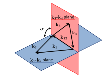
Figure 3: definition of $\alpha$

The shape correlations among the models are summarised in Table 2. In most of the models, the shape correlations based on the reduced trispectra are close to those based on the full trispectra. Especially, if the correlation based on the reduced trispectra is high, there is a little difference between the two shape correlations. Thus as long as the shape correlation is high, it is possible to use the reduced trispectrum to calculate the shape correlation. On the other hand, a care must be taken if the correlation is low.

IV Theoretical predictions and observational constraints

In this section, in order to constrain the model parameters from the amplitude of the trispectrum, we will calculate the amplitude of the estimators $g_{\rm NL}^{equil}$ based on the shape $S_{\cal T}^{c1}$ (see Eq. (35)), which can be written in a separable form Chen:2009bc . We also discuss the amplitude of the trispectrum in the regular tetrahedron limit, $t_{\rm NL}$ and the maximally symmetric configuration, $\tau_{\rm NL}$.

IV.1 $g_{\rm NL}^{equil}$

Here, following Ref. Mizuno:2010by , we discuss the theoretical predictions for the amplitude of the trispectrum $g_{\rm NL}^{equil}$. We first define the equilateral shape using $S_{\cal T}^{c1}$,

$$S_{\cal T}^{equil}=\frac{64}{3}(2\pi^{2}{\cal P}_{\zeta})^{3}S_{\cal T}^{c1},$$ (14)

where ${\cal P}_{\zeta}$ is defined as $\left\langle\zeta({\bf k}_{1})\zeta_{(}{\bf k}_{2})\right\rangle=16\pi^{5}\delta^{3}({\bf k}_{1}+{\bf k}_{2})k_{1}^{-3}{\cal P}_{\zeta}$. The parameter $g_{\rm NL}^{equil}$ is defined as the normalised shape correlation between $S_{\cal T}$ and $S_{\cal T}^{equil}$;

$$g_{\rm NL}^{equil}\equiv\frac{F(S_{\cal T},S_{\cal T}^{equil})}{F(S_{\cal T}^{equil},S_{\cal T}^{equil})}.$$ (15)

We explicitly calculate $g_{\rm NL}^{equil}$ in single field DBI inflation model, multi-field DBI inflation model, ghost inflation model and Lifshitz scalar model. The results are summarised in Table 3. Since we have two kinds of the shape correlators (one is based on the reduced trispectrum and the other is based on the full trispectrum), we show the two results in Table 3. Here, we use the fact that the power specrta of the primordial perturbations in single field and multi-field DBI inflation models, ghost inflation model and Lifshitz scalar model are given by

$$\mathcal{P}_{\zeta}^{\sigma}=\frac{1}{2\pi^{2}}\frac{H^{4}}{2\dot{\phi}^{2}},$$ (16)

$$\mathcal{P}_{\zeta}^{s}=\frac{1}{2\pi^{2}}\frac{H^{4}T_{\cal RS}}{2\dot{\phi}^{2}},$$ (17)

$$\mathcal{P}_{\zeta}^{ghost}=\frac{1}{\pi\left(\Gamma(1/4)\right)^{2}\alpha^{3/4}}\left(\frac{H}{M}\right)^{\frac{5}{2}},$$ (18)

$$\mathcal{P}_{\zeta}^{h}=\frac{1}{2\pi^{2}}\frac{M^{2}}{2\mu^{2}}.$$ (19)

Moreover, in Lifshitz scalar model, we individually show the contributions from each shape function.

Notice that although we obtain $g_{\rm NL}^{equil}$ for all theoretical models mentioned above, this $g_{\rm NL}^{equil}$ can be meaningful only in the case where the shape correlation with the equilateral shape is sufficiently high, like $>0.7$. Otherwise, this template based on the equilateral shape $S_{\cal T}^{equil}$ does not fit the shape of the trispectrum well and the noise dominates over the signal .

From this table, we find that there are little differences between $g_{\rm NL}^{equil}$ based on the reduced trispectrum and that based on the full trispectrum in most of shape functions, especially for $S_{\cal T}^{DBI(\sigma)}$, $S_{\cal T}^{h(se,12)}$ and $S_{\cal T}^{h(se,22)}$ where the shape correlation with $S_{\cal T}^{equil}$ is high enough and the use of $g_{\rm NL}^{equil}$ to measure the amplitude is justified.

Table 3: The value of $g_{\rm NL}^{equil}$ based on reduced trispectrum and full trispectrum.

	$S^{DBI(\sigma)}_{T}$	$S^{DBI(s)}_{T}$	$S^{ghost}_{T}$	$S^{h(se,11)}_{T}$	$S^{h(se,12)}_{T}$
reduced	$1.4\times 10\frac{1}{c_{s}^{4}}$	$2.3\frac{1}{c_{s}^{4}T_{\cal RS}^{2}}$	$4.9\times 10^{5}\frac{\tilde{\gamma}}{\alpha^{8/5}}\left(\frac{\mathcal{P}_{\zeta}^{1/2}}{4.8\times 10^{-5}}\right)^{-8/5}$	$1.6\times 10^{7}b_{1}^{2}\left(\frac{\mathcal{P}_{\zeta}^{1/2}}{4.8\times 10^{-5}}\right)^{-2}$	$-1.8\times 10^{8}b_{1}b_{2}\left(\frac{\mathcal{P}_{\zeta}^{1/2}}{4.8\times 10^{-5}}\right)^{-2}$
full	$1.3\times 10\frac{1}{c_{s}^{4}}$	$2.7\frac{1}{c_{s}^{4}T_{\cal RS}^{2}}$	$6.0\times 10^{5}\frac{\tilde{\gamma}}{\alpha^{8/5}}\left(\frac{\mathcal{P}_{\zeta}^{1/2}}{4.8\times 10^{-5}}\right)^{-8/5}$	$1.1\times 10^{7}b_{1}^{2}\left(\frac{\mathcal{P}_{\zeta}^{1/2}}{4.8\times 10^{-5}}\right)^{-2}$	$-1.6\times 10^{8}b_{1}b_{2}\left(\frac{\mathcal{P}_{\zeta}^{1/2}}{4.8\times 10^{-5}}\right)^{-2}$

	$S^{h(se,22)}_{T}$	$S^{h(ci,1)}_{T}$	$S^{h(ci,2)}_{T}$	$S^{h(ci,3)}_{T}$
reduced	$4.5\times 10^{8}b_{2}^{2}\left(\frac{\mathcal{P}_{\zeta}^{1/2}}{4.8\times 10^{-5}}\right)^{-2}$	$9.1\times 10^{7}t_{1}\left(\frac{\mathcal{P}_{\zeta}^{1/2}}{4.8\times 10^{-5}}\right)^{-2}$	$2.0\times 10^{8}t_{2}\left(\frac{\mathcal{P}_{\zeta}^{1/2}}{4.8\times 10^{-5}}\right)^{-2}$	$3.7\times 10^{8}t_{3}\left(\frac{\mathcal{P}_{\zeta}^{1/2}}{4.8\times 10^{-5}}\right)^{-2}$
full	$4.3\times 10^{8}b_{2}^{2}\left(\frac{\mathcal{P}_{\zeta}^{1/2}}{4.8\times 10^{-5}}\right)^{-2}$	$9.3\times 10^{7}t_{1}\left(\frac{\mathcal{P}_{\zeta}^{1/2}}{4.8\times 10^{-5}}\right)^{-2}$	$2.2\times 10^{8}t_{2}\left(\frac{\mathcal{P}_{\zeta}^{1/2}}{4.8\times 10^{-5}}\right)^{-2}$	$6.2\times 10^{7}t_{3}\left(\frac{\mathcal{P}_{\zeta}^{1/2}}{4.8\times 10^{-5}}\right)^{-2}$

IV.2 $t_{\rm NL}$ and $\tau_{NL}$

In order to estimate the amplitude of the trispectrum with different shapes, Chen et al. Chen:2009bc define the amplitude of the trispectrum $t_{\rm NL}$ using a particular configuration as follows;

$$\langle\zeta^{4}\rangle\to(2\pi)^{9}\mathcal{P}_{\zeta}^{3}\delta^{3}(\sum_{i}{\mathbb{k}_{i}})\frac{1}{k^{9}}t_{\rm NL},$$ (20)

where the limit stands for the regular tetrahedron limit $(k_{1}=k_{2}=k_{3}=k_{4}=k_{12}=k_{13}=k)$. Theoretical predictions for $t_{\rm NL}$ are summarised in Tables 4.

It is clear that $t_{\rm NL}$ gives only a rough estimation of the amplitude of the trispectrum as it is obtained by using only one specific configuration. In fact, for $S^{h(ci,3)}_{T}$, $t_{\rm NL}$ is $0$ because $S^{h(ci,3)}_{T}$ happens to vanish for the configuration given by $(k_{1}=k_{2}=k_{3}=k_{4}=k_{12}=k_{13}=k)$. On the other hand, if we consider all the configurations, there is a small but non-negligible over-lap between this shape and $S_{\cal T}^{c1}$. This clearly demonstrates that it is necessary to use all the configurations to estimate the amplitude of the trispectrum.

We also show the amplitude of the trispectrum in another definition. The configuration $(k_{1}=k_{2}=k_{3}=k_{4}=k$ and $k_{12}=k_{13}=k_{14}=2k/\sqrt{3})$ is maximally symmetric while the configuration of tetrahedron is not invariant under interchange of $\bf k_{1}$ and $\bf k_{2}$. Therefore, the maximally symmetric configuration is probably useful to analyze the trispectrum. Here, we define the amplitude of the trispectrum $\tau_{\rm NL}$ as in Arroja:2009pd ;

$$\tau_{NL}=\frac{2}{9\sqrt{3}}k^{9}\frac{T_{\zeta}}{(2\pi^{2}{\mathcal{P}_{\zeta}})^{3}},$$ (21)

where $T_{\zeta}$ is the trispectrum of the maximally symmetric configuration. Theoretial predictions for $\tau_{NL}$ are also summarised in Tables 4.

Table 4: The value of $t_{\rm NL}$ and $\tau_{NL}$.

	$S^{DBI(\sigma)}_{T}$	$S^{DBI(s)}_{T}$	$S^{ghost}_{T}$	$S^{h(se,11)}_{T}$	$S^{h(se,12)}_{T}$
$t_{\rm NL}$	$5.4\times 10^{-1}\frac{1}{c_{s}^{4}}$	$1.4\times 10^{-1}\frac{1}{c_{s}^{4}T_{\cal RS}^{2}}$	$-1.2\times 10^{5}\frac{\tilde{\gamma}}{\alpha^{8/5}}\left(\frac{\mathcal{P}_{\zeta}^{1/2}}{4.8\times 10^{-5}}\right)^{-8/5}$	$5.1\times 10^{6}b_{1}^{2}\left(\frac{\mathcal{P}_{\zeta}^{1/2}}{4.8\times 10^{-5}}\right)^{-2}$	$-2.3\times 10^{7}b_{1}b_{2}\left(\frac{\mathcal{P}_{\zeta}^{1/2}}{4.8\times 10^{-5}}\right)^{-2}$
$\tau_{\rm NL}$	$5.6\times 10^{-1}\frac{1}{c_{s}^{4}}$	$1.2\times 10^{-1}\frac{1}{c_{s}^{4}T_{\cal RS}^{2}}$	$-1.0\times 10^{4}\frac{\tilde{\gamma}}{\alpha^{8/5}}\left(\frac{\mathcal{P}_{\zeta}^{1/2}}{4.8\times 10^{-5}}\right)^{-8/5}$	$1.2\times 10^{7}b_{1}^{2}\left(\frac{\mathcal{P}_{\zeta}^{1/2}}{4.8\times 10^{-5}}\right)^{-2}$	$-9.9\times 10^{7}b_{1}b_{2}\left(\frac{\mathcal{P}_{\zeta}^{1/2}}{4.8\times 10^{-5}}\right)^{-2}$

	$S^{h(se,22)}_{T}$	$S^{h(ci,1)}_{T}$	$S^{h(ci,2)}_{T}$	$S^{h(ci,3)}_{T}$
$\tau_{\rm NL}$	$2.8\times 10^{7}b_{2}^{2}\left(\frac{\mathcal{P}_{\zeta}^{1/2}}{4.8\times 10^{-5}}\right)^{-2}$	$2.7\times 10^{6}t_{1}\left(\frac{\mathcal{P}_{\zeta}^{1/2}}{4.8\times 10^{-5}}\right)^{-2}$	$6.9\times 10^{5}t_{2}\left(\frac{\mathcal{P}_{\zeta}^{1/2}}{4.8\times 10^{-5}}\right)^{-2}$	0
$t_{\rm NL}$	$2.1\times 10^{8}b_{2}^{2}\left(\frac{\mathcal{P}_{\zeta}^{1/2}}{4.8\times 10^{-5}}\right)^{-2}$	$2.8\times 10^{6}t_{1}\left(\frac{\mathcal{P}_{\zeta}^{1/2}}{4.8\times 10^{-5}}\right)^{-2}$	$3.1\times 10^{5}t_{2}\left(\frac{\mathcal{P}_{\zeta}^{1/2}}{4.8\times 10^{-5}}\right)^{-2}$	$3.1\times 10^{5}t_{3}\left(\frac{\mathcal{P}_{\zeta}^{1/2}}{4.8\times 10^{-5}}\right)^{-2}$

IV.3 Constraints on model parameters

Observational constraints on the equilateral non-Gaussianity were obtained from WMAP5 data by applying the estimator with the shape given by $S_{\cal T}^{c1}$ Fergusson:2010gn . The constraints on the amplitude of the trispectrum in the regular tetrahedron limit is obtained as

$$t_{\rm NL}^{equil}=(-3.11\pm 7.5)\times 10^{6}\;(68\%{\rm CL}).$$ (22)

This constraint can be converted to that on $g_{\rm NL}^{equil}$ as follows. We define the following shape function

$$S_{{\cal T}}=g_{\rm NL}^{equil}\frac{64}{3}(2\pi^{2}{\cal P}_{\zeta})^{3}S_{\cal T}^{c1},$$ (23)

which by definition gives $g_{\rm NL}^{equil}$ when we apply Eq. (15). Now using the relation between the shape function and the full trispectrum and evaluating the full trispectrum in the regular tetrahedron limit, we can calculate $t_{\rm NL}^{equil}$ for this trispectrum as

$$t_{\rm NL}^{equil}=\frac{1}{32}g_{\rm NL}^{equil}.$$ (24)

Then we obtain the constraints on $g_{\rm NL}^{equil}$ as

$$g_{\rm NL}^{equil}=(-9.95\pm 24)\times 10^{7}\;(68\%{\rm CL}).$$ (25)

From the theoretical predictions for $g_{\rm NL}^{equil}$ in various models obtained by using the full trispectrum as well as the reduced trispectrum, we can derive the constraints on model parameters as in Table 5.

Table 5: Constraints on model parameters from $g_{\rm NL}^{equil}$ in various models.

	reduced	full
$S^{DBI(\sigma)}_{T}$	$1.8\times 10^{-2}<c_{s}$	$1.7\times 10^{-2}<c_{s}$
$S^{DBI(s)}_{T}$	$1.1\times 10^{-2}<c_{s}\sqrt{T_{\cal RS}}$	$1.2\times 10^{-2}<c_{s}\sqrt{T_{\cal RS}}$
$S^{ghost}_{T}$	$-6.9\times 10^{2}<\frac{\tilde{\gamma}}{\alpha^{8/5}}\left(\frac{\mathcal{P}_{\zeta}^{1/2}}{4.8\times 10^{-5}}\right)^{-8/5}<2.9\times 10^{2}$	$-5.7\times 10^{2}<\frac{\tilde{\gamma}}{\alpha^{8/5}}\left(\frac{\mathcal{P}_{\zeta}^{1/2}}{4.8\times 10^{-5}}\right)^{-8/5}<2.3\times 10^{2}$
$S^{h(se,11)}_{T}$	$(0<)\;b_{1}^{2}\left(\frac{\mathcal{P}_{\zeta}^{1/2}}{4.8\times 10^{-5}}\right)^{-2}<8.8$	$(0<)\;b_{1}^{2}\left(\frac{\mathcal{P}_{\zeta}^{1/2}}{4.8\times 10^{-5}}\right)^{-2}<1.3\times 10$
$S^{h(se,12)}_{T}$	$-7.8\times 10^{-1}<b_{1}b_{2}\left(\frac{\mathcal{P}_{\zeta}^{1/2}}{4.8\times 10^{-5}}\right)^{-2}<1.9$	$-8.8\times 10^{-1}<b_{1}b_{2}\left(\frac{\mathcal{P}_{\zeta}^{1/2}}{4.8\times 10^{-5}}\right)^{-2}<2.1$
$S^{h(se,22)}_{T}$	$(0<)\;b_{2}^{2}\left(\frac{\mathcal{P}_{\zeta}^{1/2}}{4.8\times 10^{-5}}\right)^{-2}<3.1\times 10^{-1}$	$(0<)\;b_{2}^{2}\left(\frac{\mathcal{P}_{\zeta}^{1/2}}{4.8\times 10^{-5}}\right)^{-2}<3.3\times 10^{-1}$
$S^{h(ci,1)}_{T}$	$-3.7<t_{1}\left(\frac{\mathcal{P}_{\zeta}^{1/2}}{4.8\times 10^{-5}}\right)^{-2}<1.5$	$-3.7<t_{1}\left(\frac{\mathcal{P}_{\zeta}^{1/2}}{4.8\times 10^{-5}}\right)^{-2}<1.5$
$S^{h(ci,2)}_{T}$	$-1.7<t_{2}\left(\frac{\mathcal{P}_{\zeta}^{1/2}}{4.8\times 10^{-5}}\right)^{-2}<7.0\times 10^{-1}$	$-1.5<t_{2}\left(\frac{\mathcal{P}_{\zeta}^{1/2}}{4.8\times 10^{-5}}\right)^{-2}<6.4\times 10^{-1}$
$S^{h(ci,3)}_{T}$	$-9.2\times 10^{-1}<t_{3}\left(\frac{\mathcal{P}_{\zeta}^{1/2}}{4.8\times 10^{-5}}\right)^{-2}<3.8\times 10^{-1}$	$-5.5<t_{3}\left(\frac{\mathcal{P}_{\zeta}^{1/2}}{4.8\times 10^{-5}}\right)^{-2}<2.3$

V Summary and Discussions

There are many interesting early universe models motivated by string theory and the effective field theory that predict large primordial non-Gaussianity with the equilateral type bispectrum. Given that future experiments like Planck can prove even higher-order statistics, it is important to investigate whether the shape of the trispectrum can distinguish such equilateral type non-Gaussian models. For this purpose, the shape correlator of the trispectrum is particularly useful.

So far, the shape correlator constructed from the reduced trispectrum has been adopted Regan et al. (2010). While the reduced trispectrum has all information of the full trispectrum, the shape correlator based on the reduced trispectrum depends on the way in which the full trispectrum is decomposed into reduced trispectra because the form of the integration variables in the shape correlator breaks the transposition invariance of momenta $\bf k_{1}$, $\bf k_{2}$, $\bf k_{3}$ and $\bf k_{4}$. In most equilateral type non-Gaussian models such as DBI inflation model, there is a natural way to decompose the full trispectrum into the reduced trispectra so that one of the reduced trispectra depends only on five parameters $k_{1}$, $k_{2}$, $k_{3}$, $k_{4}$ and $k_{12}$. However, for some classes of equilateral type non-Gaussian model like Lifshitz scalar model, this decomposition is not possible. Therefore, in this paper, we studied the shape correlator of the primordial trispectrum based on the full trispectrum.

In order to check the difference between the two shape correlators, we calculated the shape correlations among trispectra in various equilateral non-Gaussian models; DBI inflation, ghost inflation and Lifshitz scalar models. We found that both shape correlators give similar results as long as the shape correlations are high.

From the shape correlations, it is possible to judge whether we can distinguish between various equilateral non-Gaussian models using the tripsectrum. For example, we showed that it is difficult to distinguish between the single field DBI inflation model and the $b_{2}b_{2}$-dominated Lifshitz scalar model by the shape of the trispectrum. Since both single field DBI inflation model Alishahiha:2004eh and $b_{2}b_{2}$-dominated Lifshitz scalar model Izumi:2010yn predict almost the same equilateral type bispectrum, we can not distinguish between these two models by the primordial non-Gaussianity up to this order. In order to distinguish between these models, we need other information such as the primordial gravitational wave. A similar conclusion holds for the comparison between the ghost inflation model and $t_{1}$-dominated Lifshitz scalar model. Despite these exceptions, our result suggests that we can distinguish between many equilateral non-Gaussian models, which predict almost the same equilateral type bispectrum, from the shape of the trispectrum.

On the other hand, in order to measure the amplitude of the trispectrum and constrain parameters in the theoretical models, it is necessary to develop an estimator for the trispectrum. Since the form of the trispectrum is too complicated for this class of models, it is generally impossible to construct an optimal estimator (see however Regan et al. (2010) for the model independent approach). Using the fact that the shape $S_{\mathcal{T}}^{c1}$ given by Eq. (35) can be written as a separable form, it is possible to construct a fast optimal estimator $g_{\rm NL}^{equil}$ Mizuno:2010by ; Fergusson:2010gn . We expressed the estimator in terms of models parameters in various models. The constraint on $g_{\rm NL}^{equil}$ was obtained from WMAP5 in Fergusson:2010gn . From this constraint, we obtained constraints on model parameters. We emphasized that the amplitude of the trispectrum for a particular configuration such as the regular tetrahedron limit cannot be reliably used to characterise the amplitude of the trispectrum and we need to use all configurations to define the amplitude $g_{\rm NL}^{equil}$.

Finally, it is known that that inflation models based on Galileon and its generalisations, which are shown to be the most general single field inflation model with second-order field equations Kobayashi:2011nu ; Charmousis:2011bf give also the equilateral type bispectrum Mizuno:2010ag ; Burrage:2010cu ; Creminelli:2010qf ; Kobayashi:2011pc ; RenauxPetel:2011dv ; RenauxPetel:2011uk ; Gao:2011qe ; DeFelice:2011uc (see also for the discussion about the shape dependence of the bispectrum in this type of inflation model RenauxPetel:2011sb ). It would be interesting to study the amplitude of the trispectrum $g_{\rm NL}^{equil}$ in these models.

Appendix A Shape functions in general single field k-inflation

Here, based on our previous work Arroja:2009pd , we summarise the shape functions for the reduced trispectra in general single field k-inflation models described by the following action:

$$S=\frac{1}{2}\int d^{4}x\sqrt{-g}\left[R+2P(X,\phi)\right],$$ (26)

where $\phi$ is the inflaton field, $R$ is the Ricci scalar and $X\equiv-(1/2)g^{\mu\nu}\partial_{\mu}\phi\partial_{\nu}\phi$, where $g_{\mu\nu}$ is the metric tensor.

In this class of models, the third and the fourth order interaction Hamiltonian of the field perturbation $\delta\phi$ in the flat gauge at leading order in the slow-roll expansion are given by

$$H_{I}^{(3)}(\eta) = \int d^{3}x\left[Aa\delta\phi^{\prime 3}+Ba\delta\phi^{\prime}\left(\partial\delta\phi\right)^{2}\right]\,,$$ (27)

$$H_{I}^{(4)}(\eta) = \int d^{3}x\left[\beta_{1}\delta\phi^{\prime 4}+\beta_{2}\delta\phi^{\prime 2}\left(\partial\delta\phi\right)^{2}+\beta_{3}\left(\partial\delta\phi\right)^{4}\right]\,,$$ (28)

where prime denotes derivative with respect to conformal time $\eta$ and coefficients $A$, $B$, $\beta_{1}$, $\beta_{2}$ and $\beta_{3}$ are given by

$$A=-\frac{\sqrt{2X}}{2}\left(P_{,XX}+\frac{2}{3}XP_{,XXX}\right),\quad B=\frac{\sqrt{2X}}{2}P_{,XX}.$$ (29)

$$\beta_{1} = P_{,XX}\left(1-\frac{9}{8}c_{s}^{2}\right)-2XP_{,XXX}\left(1-\frac{3}{4}c_{s}^{2}\right)+\frac{X^{3}c_{s}^{2}}{P_{,X}}P_{,XXX}^{2}-\frac{1}{6}X^{2}P_{,4X},$$

$$\beta_{2} = -\frac{1}{2}P_{,XX}\left(1-\frac{3}{2}c_{s}^{2}\right)+\frac{1}{2}Xc_{s}^{2}P_{,XXX},$$

$$\beta_{3} = -\frac{c_{s}^{2}}{8}P_{,XX}.$$ (30)

Here, $P_{,X}$ denotes the derivative of $P$ with respect to $X$, $P_{,XX}$ denotes the second derivative of $P$ with respect to $X$, and so on. $c_{s}$ is the sound speed of the perturbation of the scalar field $\phi$ which is defined as

$$c_{s}^{2}\equiv\frac{P_{,X}}{P_{,X}+2XP_{,XX}}.$$ (31)

The shape function $S^{k}_{T}$ is composed of two parts

$$S^{k}_{T}=S^{k(cont)}_{T}+S^{k(scalar)}_{T}\,,$$ (32)

where $S^{k(cont)}_{T}$ denotes the contribution from the contact interaction and $S^{k(scalar)}_{T}$ denotes that from the scalar exchange interaction, respectively.

The shape function for the reduced trispectrum arising from the contact interaction $S^{k(cont)}_{\mathcal{T}}$ depend on five parameters $k_{1}$, $k_{2}$, $k_{3}$, $k_{4}$ and $k_{12}$. It is given by

$$S^{k(cont)}_{\mathcal{T}}=\left(-24\beta_{1}c_{s}^{3}S^{c_{1}}_{\mathcal{T}}-\beta_{2}c_{s}S^{c_{2}}_{\mathcal{T}}-2\beta_{3}c_{s}^{-1}S^{c_{3}}_{\mathcal{T}}\right)\frac{H^{4}}{4X^{2}}N^{8}\,.$$ (33)

Here $S^{c_{1}}_{\mathcal{T}}$, $S^{c_{2}}_{\mathcal{T}}$ and $S^{c_{3}}_{\mathcal{T}}$ are the following shape functions:

$$S^{c_{1}}_{\mathcal{T}} = \frac{k_{12}\Pi_{i=1}^{4}k_{i}}{\left(\sum_{i=1}^{4}k_{i}\right)^{5}}+3\;\;{\rm perms.}\,,$$ (34)

$$S^{c_{2}}_{\mathcal{T}} = \Biggl{[}\frac{k_{12}k_{1}^{2}k_{2}^{2}(\mathbf{k_{3}}\cdot\mathbf{k_{4}})}{\left(\sum_{i=1}^{4}k_{i}\right)^{3}\Pi_{i=1}^{4}k_{i}}\left(1+3\frac{(k_{3}+k_{4})}{\sum_{i=1}^{4}k_{i}}+12\frac{k_{3}k_{4}}{\left(\sum_{i=1}^{4}k_{i}\right)^{2}}\right)$$ (35)

$$+\frac{k_{12}k_{3}^{2}k_{4}^{2}(\mathbf{k_{1}}\cdot\mathbf{k_{2}})}{\left(\sum_{i=1}^{4}k_{i}\right)^{3}\Pi_{i=1}^{4}k_{i}}\left(1+3\frac{(k_{1}+k_{2})}{\sum_{i=1}^{4}k_{i}}+12\frac{k_{1}k_{2}}{\left(\sum_{i=1}^{4}k_{i}\right)^{2}}\right)\Biggr{]}+3\;\;{\rm perms.}\,,$$

$$S^{c_{3}}_{\mathcal{T}} = \frac{k_{12}(\mathbf{k_{1}}\cdot\mathbf{k_{2}})(\mathbf{k_{3}}\cdot\mathbf{k_{4}})}{\sum_{i=1}^{4}k_{i}\,\Pi_{i=1}^{4}k_{i}}\left(1+\frac{\sum_{i<j}k_{i}k_{j}}{\left(\sum_{i=1}^{4}k_{i}\right)^{2}}+3\frac{\Pi_{i=1}^{4}k_{i}}{\left(\sum_{i=1}^{4}k_{i}\right)^{3}}\sum_{i=1}^{4}\frac{1}{k_{i}}+12\frac{\Pi_{i=1}^{4}k_{i}}{\left(\sum_{i=1}^{4}k_{i}\right)^{4}}\right)+3\;\;{\rm perms.}\,,$$ (36)

where “$3\;\;{\rm perms.}$” denotes the permutations $(k_{1}\leftrightarrow k_{2})$, $(k_{3}\leftrightarrow k_{4})$ and $(k_{1}\leftrightarrow k_{2},k_{3}\leftrightarrow k_{4})$. In Eq. (33), $H$ is the Hubble parameter at inflation era and $N=H/\sqrt{2P_{,X}c_{s}}$.

Similarly, $S^{k(scalar)}_{\mathcal{T}}$ is given by

$$S^{k(scalar)}_{\mathcal{T}}=\left(A^{2}c_{s}^{4}S^{s_{1}}_{\mathcal{T}}+ABc_{s}^{2}S^{s_{3}}_{\mathcal{T}}+B^{2}S^{s_{2}}_{\mathcal{T}}\right)\frac{c_{s}^{2}H^{2}N^{10}}{8X^{2}}\,.$$ (37)

Here $S^{s_{1}}_{\mathcal{T}}$, $S^{s_{2}}_{\mathcal{T}}$ and $S^{s_{3}}_{\mathcal{T}}$ are the following shape functions:

$$S^{s_{1}}_{\mathcal{T}} = -9k_{12}(k_{1}k_{2}k_{3}k_{4})^{1/2}\biggl{[}\tilde{\mathcal{F}}_{1}(k_{1},k_{2},-k_{12},k_{3},k_{4},k_{12})-\tilde{\mathcal{F}}_{1}(-k_{1},-k_{2},-k_{12},k_{3},k_{4},k_{12})$$ (38)

$$+\tilde{\mathcal{F}}_{1}(k_{3},k_{4},-k_{12},k_{1},k_{2},k_{12})-\tilde{\mathcal{F}}_{1}(-k_{3},-k_{4},-k_{12},k_{3},k_{4},k_{12})\biggr{]}+3\;\;{\rm perms.}\,,$$

$$S^{s_{2}}_{\mathcal{T}} = S^{s_{2a}}_{\mathcal{T}}+S^{s_{2b}}_{\mathcal{T}}+S^{s_{2c}}_{\mathcal{T}}+S^{s_{2d}}_{\mathcal{T}}\,,$$ (39)

$$S^{s_{2a}}_{\mathcal{T}} = -k_{12}(k_{1}k_{2}k_{3}k_{4})^{1/2}(\mathbf{k_{1}}\cdot\mathbf{k_{2}})(\mathbf{k_{3}}\cdot\mathbf{k_{4}})\biggl{[}\tilde{\mathcal{F}}_{2}(-k_{12},k_{1},k_{2},k_{12},k_{3},k_{4})-\tilde{\mathcal{F}}_{2}(-k_{12},-k_{1},-k_{2},k_{12},k_{3},k_{4})$$ (40)

$$+\tilde{\mathcal{F}}_{2}(-k_{12},k_{3},k_{4},k_{12},k_{1},k_{2})-\tilde{\mathcal{F}}_{2}(-k_{12},-k_{3},-k_{4},k_{12},k_{1},k_{2})\biggr{]}+3\;\;{\rm perms.}\,,$$

$$S^{s_{2b}}_{\mathcal{T}} = -2k_{12}(k_{1}k_{2}k_{3}k_{4})^{1/2}(\mathbf{k_{1}}\cdot\mathbf{k_{2}})(\mathbf{k_{12}}\cdot\mathbf{k_{4}})\biggl{[}\tilde{\mathcal{F}}_{2}(-k_{12},k_{1},k_{2},k_{3},k_{4},k_{12})-\tilde{\mathcal{F}}_{2}(-k_{12},-k_{1},-k_{2},k_{3},k_{4},k_{12})$$ (41)

$$+\tilde{\mathcal{F}}_{2}(k_{3},k_{4},-k_{12},k_{12},k_{1},k_{2})-\tilde{\mathcal{F}}_{2}(-k_{3},-k_{4},-k_{12},k_{12},k_{1},k_{2})\biggr{]}+3\;\;{\rm perms.}\,,$$

$$S^{s_{2c}}_{\mathcal{T}} = 2k_{12}(k_{1}k_{2}k_{3}k_{4})^{1/2}(\mathbf{k_{12}}\cdot\mathbf{k_{2}})(\mathbf{k_{3}}\cdot\mathbf{k_{4}})\biggl{[}\tilde{\mathcal{F}}_{2}(k_{1},k_{2},-k_{12},k_{12},k_{3},k_{4})-\tilde{\mathcal{F}}_{2}(-k_{1},-k_{2},-k_{12},k_{12},k_{3},k_{4})$$ (42)

$$+\tilde{\mathcal{F}}_{2}(-k_{12},k_{3},k_{4},k_{1},k_{2},k_{12})-\tilde{\mathcal{F}}_{2}(-k_{12},-k_{3},-k_{4},k_{1},k_{2},k_{12})\biggr{]}+3\;\;{\rm perms.}\,,$$

$$S^{s_{2d}}_{\mathcal{T}} = 4k_{12}(k_{1}k_{2}k_{3}k_{4})^{1/2}(\mathbf{k_{12}}\cdot\mathbf{k_{2}})(\mathbf{k_{12}}\cdot\mathbf{k_{4}})\biggl{[}\tilde{\mathcal{F}}_{2}(k_{1},k_{2},-k_{12},k_{3},k_{4},k_{12})-\tilde{\mathcal{F}}_{2}(-k_{1},-k_{2},-k_{12},k_{3},k_{4},k_{12})$$ (43)

$$+\tilde{\mathcal{F}}_{2}(k_{3},k_{4},-k_{12},k_{1},k_{2},k_{12})-\tilde{\mathcal{F}}_{2}(-k_{3},-k_{4},-k_{12},k_{1},k_{2},k_{12})\biggr{]}+3\;\;{\rm perms.}\,,$$

$$S^{s_{3}}_{\mathcal{T}} = S^{s_{3a}}_{\mathcal{T}}+S^{s_{3b}}_{\mathcal{T}}+S^{s_{3c}}_{\mathcal{T}}+S^{s_{3d}}_{\mathcal{T}}\,,$$ (44)

$$S^{s_{3a}}_{\mathcal{T}} = 3k_{12}(k_{1}k_{2}k_{3}k_{4})^{1/2}(\mathbf{k_{3}}\cdot\mathbf{k_{4}})\biggl{[}\tilde{\mathcal{F}}_{3}(k_{1},k_{2},-k_{12},k_{12},k_{3},k_{4})-\tilde{\mathcal{F}}_{3}(-k_{1},-k_{2},-k_{12},k_{12},k_{3},k_{4})$$ (45)

$$+\tilde{\mathcal{F}}_{4}(-k_{12},k_{3},k_{4},k_{1},k_{2},k_{12})-\tilde{\mathcal{F}}_{4}(-k_{12},-k_{3},-k_{4},k_{1},k_{2},k_{12})\biggr{]}+3\;\;{\rm perms.}\,,$$

$$S^{s_{3b}}_{\mathcal{T}} = 6k_{12}(k_{1}k_{2}k_{3}k_{4})^{1/2}(\mathbf{k_{12}}\cdot\mathbf{k_{4}})\biggl{[}\tilde{\mathcal{F}}_{3}(k_{1},k_{2},-k_{12},k_{3},k_{4},k_{12})-\tilde{\mathcal{F}}_{3}(-k_{1},-k_{2},-k_{12},k_{3},k_{4},k_{12})$$ (46)

$$+\tilde{\mathcal{F}}_{4}(k_{3},k_{4},-k_{12},k_{1},k_{2},k_{12})-\tilde{\mathcal{F}}_{4}(-k_{3},-k_{4},-k_{12},k_{1},k_{2},k_{12})\biggr{]}+3\;\;{\rm perms.}\,,$$

$$S^{s_{3c}}_{\mathcal{T}} = 3k_{12}(k_{1}k_{2}k_{3}k_{4})^{1/2}(\mathbf{k_{1}}\cdot\mathbf{k_{2}})\biggl{[}\tilde{\mathcal{F}}_{4}(-k_{12},k_{1},k_{2},k_{3},k_{4},k_{12})-\tilde{\mathcal{F}}_{4}(-k_{12},-k_{1},-k_{2},k_{3},k_{4},k_{12})$$ (47)

$$+\tilde{\mathcal{F}}_{3}(k_{3},k_{4},-k_{12},k_{12},k_{1},k_{2})-\tilde{\mathcal{F}}_{3}(-k_{3},-k_{4},-k_{12},k_{12},k_{1},k_{2})\biggr{]}+3\;\;{\rm perms.}\,,$$

$$S^{s_{3d}}_{\mathcal{T}} = -6k_{12}(k_{1}k_{2}k_{3}k_{4})^{1/2}(\mathbf{k_{12}}\cdot\mathbf{k_{2}})\biggl{[}\tilde{\mathcal{F}}_{4}(k_{1},k_{2},-k_{12},k_{3},k_{4},k_{12})-\tilde{\mathcal{F}}_{4}(-k_{1},-k_{2},-k_{12},k_{3},k_{4},k_{12})$$ (48)

$$+\tilde{\mathcal{F}}_{3}(k_{3},k_{4},-k_{12},k_{1},k_{2},k_{12})-\tilde{\mathcal{F}}_{3}(-k_{3},-k_{4},-k_{12},k_{1},k_{2},k_{12})\biggr{]}+3\;\;{\rm perms.}\,,$$

where again “$3\;\;{\rm perms.}$” denotes the permutations $(k_{1}\leftrightarrow k_{3})$, $(k_{3}\leftrightarrow k_{4})$ and $(k_{1}\leftrightarrow k_{2},k_{3}\leftrightarrow k_{4})$. Here we have defined four $\tilde{\mathcal{F}}_{i}$ functions (with $i=1,\ldots,4$) as follows;

$$\tilde{\mathcal{F}}_{1}(k_{1},k_{2},k_{3},k_{4},k_{5},k_{6}) = -4|k_{1}k_{2}k_{3}k_{4}k_{5}k_{6}|^{\frac{1}{2}}\frac{1}{\mathcal{A}^{3}\mathcal{C}^{3}}\left(1+3\frac{\mathcal{A}}{\mathcal{C}}+6\frac{\mathcal{A}^{2}}{\mathcal{C}^{2}}\right)\,,$$ (49)

$$\tilde{\mathcal{F}}_{2}(k_{1},k_{2},k_{3},k_{4},k_{5},k_{6}) = -\frac{|k_{1}k_{4}|^{\frac{1}{2}}}{|k_{2}k_{3}k_{5}k_{6}|^{\frac{3}{2}}}\frac{1}{\mathcal{A}\mathcal{C}}\bigg{[}1+\frac{k_{5}+k_{6}}{\mathcal{A}}+2\frac{k_{5}k_{6}}{\mathcal{A}^{2}}$$ (50)

$$+\frac{1}{\mathcal{C}}\left(k_{2}+k_{3}+k_{5}+k_{6}+\frac{1}{\mathcal{A}}\left(\left(k_{2}+k_{3}\right)\left(k_{5}+k_{6}\right)+2k_{5}k_{6}\right)+2\frac{k_{5}k_{6}\left(k_{2}+k_{3}\right)}{\mathcal{A}^{2}}\right)$$

$$+\frac{2}{\mathcal{C}^{2}}\bigl{(}k_{5}k_{6}+\left(k_{2}+k_{3}\right)\left(k_{5}+k_{6}\right)+k_{2}k_{3}+\frac{1}{\mathcal{A}}\left(k_{2}k_{3}\left(k_{5}+k_{6}\right)+2k_{5}k_{6}\left(k_{2}+k_{3}\right)\right)$$

$$+2\frac{k_{2}k_{3}k_{5}k_{6}}{\mathcal{A}^{2}}\bigr{)}+\frac{6}{\mathcal{C}^{3}}\left(k_{2}k_{3}\left(k_{5}+k_{6}\right)+k_{5}k_{6}\left(k_{2}+k_{3}\right)+2\frac{k_{2}k_{3}k_{5}k_{6}}{\mathcal{A}}\right)$$

$$+24\frac{k_{2}k_{3}k_{5}k_{6}}{\mathcal{C}^{4}}\bigg{]}\,,$$

$$\tilde{\mathcal{F}}_{3}(k_{1},k_{2},k_{3},k_{4},k_{5},k_{6}) = 2\frac{|k_{1}k_{2}k_{3}k_{4}|^{\frac{1}{2}}}{|k_{5}k_{6}|^{\frac{3}{2}}}\frac{1}{\mathcal{A}\mathcal{C}^{3}}\left[1+\frac{k_{5}+k_{6}}{\mathcal{A}}+2\frac{k_{5}k_{6}}{\mathcal{A}^{2}}+\frac{3}{\mathcal{C}}\left(k_{5}+k_{6}+2\frac{k_{5}k_{6}}{\mathcal{A}}\right)+12\frac{k_{5}k_{6}}{\mathcal{C}^{2}}\right]\,,$$ (51)

$$\tilde{\mathcal{F}}_{4}(k_{1},k_{2},k_{3},k_{4},k_{5},k_{6}) = 2\frac{|k_{1}k_{4}k_{5}k_{6}|^{\frac{1}{2}}}{|k_{2}k_{3}|^{\frac{3}{2}}}\frac{1}{\mathcal{A}^{3}\mathcal{C}}\bigg{[}1+\frac{\mathcal{A}}{\mathcal{C}}+\frac{\mathcal{A}^{2}}{\mathcal{C}^{2}}+\frac{k_{2}+k_{3}}{\mathcal{C}}+2\frac{\mathcal{A}\left(k_{2}+k_{3}\right)+k_{2}k_{3}}{\mathcal{C}^{2}}$$ (52)

$$\qquad\qquad\qquad\qquad\qquad\quad+3\frac{\mathcal{A}}{\mathcal{C}^{3}}\left(\mathcal{A}\left(k_{2}+k_{3}\right)+2k_{2}k_{3}\right)+12k_{2}k_{3}\frac{\mathcal{A}^{2}}{\mathcal{C}^{4}}\bigg{]}\,,$$

where $\mathcal{A}$ is defined by the sum of the last three arguments of the $\tilde{\mathcal{F}}_{i}$ functions as $\mathcal{A}=k_{4}+k_{5}+k_{6}$ and $\mathcal{C}$ is defined by the sum of all the arguments as $\mathcal{C}=k_{1}+k_{2}+k_{3}+k_{4}+k_{5}+k_{6}$.

To simplify the calculation, it is useful to notice that the following properties

$$F(S^{c_{1}}_{\mathcal{T}},\;S_{\mathcal{T}}) = \sum_{i}a_{i}F(S^{c_{1}}_{\mathcal{T}},\;S^{i}_{\mathcal{T}})\,,$$ (53)

$$F(S_{\mathcal{T}},\;S_{\mathcal{T}}) = \sum_{i,j}a_{i}a_{j}F(S^{i}_{\mathcal{T}},\;S^{j}_{\mathcal{T}})\,,$$ (54)

hold for the shape function given by

$$S_{\mathcal{T}}=\sum_{i}a_{i}S^{i}_{\mathcal{T}}\,,$$ (55)

where $i=c_{1},c_{2},c_{3},s_{1},s_{2},s_{3}$ and $a_{i}$’s are corresponding coefficients.

Especially, in the case of single field DBI inflation, the coefficients in the Hamiltonians (27) and (28) are given by

$$A=-\frac{1}{2\dot{\phi}c_{s}^{5}}\,,\;\;\;\;B=\frac{1}{2\dot{\phi}c_{s}^{3}}\,,$$

$$\beta_{1}=\frac{1}{2c_{s}^{7}\dot{\phi}^{2}}\,,\;\;\;\;\beta_{2}=\frac{1}{4c_{s}^{3}\dot{\phi}^{2}}\,,\;\;\;\;\beta_{3}=-\frac{1}{8c_{s}\dot{\phi}^{2}}\,,$$ (56)

and then the shape function based on the reduced trispectrum becomes

$$S_{\mathcal{T}}^{DBI(\sigma)}=\frac{H^{12}}{{\dot{\phi}}^{6}c_{s}^{4}}\left[-3S_{\mathcal{T}}^{c1}+\frac{1}{64}S_{\mathcal{T}}^{s1}+\frac{1}{64}S_{\mathcal{T}}^{s2}-\frac{1}{64}S_{\mathcal{T}}^{s3}\right]\,.$$ (57)

In multi-field DBI inflation model Mizuno:2009mv , in addition to the shape functions $S^{c_{1}}_{\mathcal{T}}$, $S^{c_{2}}_{\mathcal{T}}$, $S^{c_{3}}_{\mathcal{T}}$, $S^{s_{1}}_{\mathcal{T}}$ $S^{s_{2}}_{\mathcal{T}}$, $S^{s_{3}}_{\mathcal{T}}$, we find it convenient to define the following shape functions $S^{\tilde{s}_{2}}_{\mathcal{T}}$ and $S^{\tilde{s}_{3}}_{\mathcal{T}}$ given by

$$S^{\tilde{s}_{2}}_{\mathcal{T}} = S^{s_{2a}}_{\mathcal{T}}-S^{s_{2b}}_{\mathcal{T}}-S^{s_{2c}}_{\mathcal{T}}+S^{s_{2d}}_{\mathcal{T}}\,,$$ (58)

$$S^{\tilde{s}_{3}}_{\mathcal{T}} = S^{s_{3a}}_{\mathcal{T}}-S^{s_{3b}}_{\mathcal{T}}+S^{s_{3c}}_{\mathcal{T}}-S^{s_{3d}}_{\mathcal{T}}\,.$$ (59)

With the above functions, the shape function based on the reduced trispectrum of the multi-field DBI inflation model can be expressed as

$$S_{\mathcal{T}}^{DBI(s)}=\frac{H^{12}}{{\dot{\phi}}^{6}c_{s}^{4}}T_{\cal RS}\left[-\frac{1}{8}S_{\mathcal{T}}^{c2}+\frac{1}{576}S_{\mathcal{T}}^{s1}+\frac{1}{64}S_{\mathcal{T}}^{\tilde{s}_{2}}+\frac{1}{192}S_{\mathcal{T}}^{\tilde{s}_{3}}\right],$$ (60)

where $T_{\cal RS}$ is the transfer coefficient that relate the amplitude of original entropy perturbations to the final curvature perturbation .

Appendix B Shape function in ghost inflation

In this appendix, based on our paper Izumi:2010wm , we review the trispectrum in ghost inflation and summarise its shape functions. Ghost inflation is an inflation model where the inflation is driven by a scalar field $\phi$ in the ghost condensation model. The ghost condensation is the simplest Higgs phase for gravity in infrared and in this model the four dimensional diffeomorphism is spontaneously broken by the timelike vacuum expectation value of the derivative of the scalar field $\phi$. Thus, the action for the perturbative field $\pi$ of $\phi$ does not invariant under four dimensional diffeomorphism and relevant terms up to fourth order are written generally as

$$S=\int dtdx^{3}a^{3}\left[\frac{1}{2}(\partial_{t}\pi)^{2}-\frac{\alpha}{2M^{2}}\left(\frac{\vec{\nabla}^{2}}{a^{2}}\pi\right)^{2}-\frac{\beta}{2M^{2}}\partial_{t}\pi\frac{(\vec{\nabla}\pi)^{2}}{a^{2}}-\frac{\gamma}{8M^{4}}\frac{(\vec{\nabla}\pi)^{4}}{a^{4}}\right],$$ (61)

where $\alpha$, $\beta$ and $\gamma$ are dimensionless constants of order unity and $M$ is a constant with a dimension of mass. Then, interaction Hamiltonian is written as

$$H_{I}=\int dtd^{3}xa^{3}\left[\frac{\beta}{2M^{2}}\partial_{t}\pi\frac{\left({\vec{\nabla}}\pi\right)^{2}}{a^{2}}+\frac{\tilde{\gamma}}{8M^{4}}\frac{\left({\vec{\nabla}}\pi\right)^{4}}{a^{4}}\right],$$ (62)

where $\tilde{\gamma}=\gamma+2\beta^{2}$.

Trispectrum from the tree level contribution can be decomposed into two parts. One is obtained by the fourth order interaction Hamiltonian and proportional to $\tilde{\gamma}$ which is called the contact interaction contribution. The other is obtained by the product of the third order interaction Hamiltonian and independent of $\tilde{\gamma}$ which is called the scalar exchange contribution.

Here, for simplicity we work only on the contact interaction contribution of the trispectrum as only this contribution has new information related with the four-point vertex. From Eq. (62), if the condition $\gamma\gg\beta^{2}$ is satisfied, this treatment can be justified.

According to Izumi:2010wm , the shape function of the contact interaction contribution from the ghost inflation based on the reduced trispectrum can be written as

$$S_{\mathcal{T}}^{ghost} \!\!=\!\! \frac{\tilde{\gamma}}{2^{3}\alpha^{3/2}}\left(\frac{H}{M}\right)^{9}\left(\frac{\pi}{\Gamma(1/4)}\right)^{4}\left(k_{1}k_{2}k_{3}k_{4}\right)^{1/2}k_{12}({\bf k_{1}}\cdot{\bf k_{2}})({\bf k_{3}}\cdot{\bf k_{4}})$$ (63)

$$\qquad\qquad\Re\biggl{\{}i\int^{0}_{-\infty}d\eta^{\prime}\left((-\eta^{\prime})^{3/2}H_{3/4}^{(1)}(q_{1}{\eta^{\prime}}^{2})\right)\left((-\eta^{\prime})^{3/2}H_{3/4}^{(1)}(q_{2}{\eta^{\prime}}^{2})\right)$$

$$\qquad\qquad\qquad\qquad\qquad\qquad\qquad\qquad\qquad\left((-\eta^{\prime})^{3/2}H_{3/4}^{(1)}(q_{3}{\eta^{\prime}}^{2})\right)\left((-\eta^{\prime})^{3/2}H_{3/4}^{(1)}(q_{4}{\eta^{\prime}}^{2})\right)\biggr{\}},$$

where $q_{i}=\sqrt{\alpha}Hk_{i}^{2}/(2M)$. Here, we choose the reduced trispectrum such that depends on the 5 parameters $k_{1}$, $k_{2}$, $k_{3}$, $k_{4}$ and $k_{12}$ as is the case in DBI inflation (see Appendix A).

Appendix C Shape function in Lifshitz scalar

In this appendix, based on our previous paper Izumi:2010yn , we derive the shape function for the trispectrum in Lifshitz scalar. Generally, some shapes of bispectra and trispectra from the Lifshitz scalar are generated because the action is not severely constrained by symmetries. As we discuss in our previous paper Izumi:2010yn , however, only the local type bispectrum stems from the term which does not have the shift symmetry. In this paper, since we want to distinguish between the models where the equilateral type bispectrum are generated, we concentrate on the model with the shift symmetry. Moreover, only in the case with the dynamical critical exponent $z=3$ we can have the scale invariant power spectrum. Thus we choose $z=3$.

The terms up to fourth order of the action of Lifshitz scalar with $z=3$ and with the shift symmetry in the ultra violet is written as

$$S=\frac{1}{2}\int dtd^{3}x\,a(t)^{3}\biggl{[}(\partial_{t}\phi)^{2}+\frac{1}{M^{4}a(t)^{6}}\phi\Delta^{3}\phi+\frac{1}{M^{5}a(t)^{6}}\left\{b_{1}(\Delta^{2}\phi)(\partial_{i}\phi)^{2}+b_{2}(\Delta\phi)^{3}\right\}$$

$$\qquad\qquad\qquad+\frac{1}{M^{6}a(t)^{6}}\left\{t_{1}\left(\Delta\phi\right)^{2}\left(\partial_{i}\phi\right)^{2}+t_{2}\left(\partial_{i}\partial_{j}\phi\right)^{2}\left(\partial_{k}\phi\right)^{2}+t_{3}(\partial_{i}\partial_{j}\partial_{k}\phi)(\partial_{i}\phi)(\partial_{j}\phi)(\partial_{k}\phi)\right\}\biggr{]},$$ (64)

where $M$, $b_{1}$, $b_{2}$, $t_{1}$, $t_{2}$ and $t_{3}$ are constants. Then, the interaction Hamiltonian conforms with the non-linear terms of the action given by Eq. (64).

We can decompose the contributions of the trispectrum into six parts which are proportional to $b_{1}^{2}$, $b_{1}b_{2}$, $b_{2}^{2}$, $t_{1}$, $t_{2}$ and $t_{3}$. The scalar exchange contributions are the first three and the others are the contact interaction contributions. According to our previous paper Izumi:2010yn , the shape functions of these contributions can be written as

$$S_{\mathcal{T}}^{h(se,ij)}=\frac{M^{4}}{2^{3}\mu^{4}}\frac{(k_{1}^{3}+k_{2}^{3}+k_{3}^{3}+k_{4}^{3}+k_{12}^{3})f_{i}(\boldsymbol{k_{1}},\boldsymbol{k_{2}})f_{j}(\boldsymbol{k_{3}},\boldsymbol{k_{4}})}{k_{1}k_{2}k_{3}k_{4}k_{12}^{2}(k_{1}^{3}+k_{2}^{3}+k_{12}^{3})(k_{3}^{3}+k_{4}^{3}+k_{12}^{3})(k_{1}^{3}+k_{2}^{3}+k_{3}^{3}+k_{4}^{3})},$$ (65)

$$S_{\mathcal{T}}^{h(ci,i)}=-\frac{M^{4}}{2^{3}\mu^{4}}\frac{k_{12}r_{i}(\boldsymbol{k_{1}},\boldsymbol{k_{2}},\boldsymbol{k_{3}},\boldsymbol{k_{4}})}{k_{1}k_{2}k_{3}k_{4}(k_{1}^{3}+k_{2}^{3}+k_{3}^{3}+k_{4}^{3})},$$ (66)

$$f_{1}(\boldsymbol{k_{i}},\boldsymbol{k_{j}})\equiv b_{1}(k_{i}^{6}+k_{j}^{6}+k_{ij}^{6}-k_{i}^{2}k_{j}^{4}-k_{i}^{4}k_{j}^{2}-k_{i}^{2}k_{ij}^{4}-k_{i}^{4}k_{ij}^{2}-k_{j}^{2}k_{ij}^{4}-k_{j}^{4}k_{ij}^{2}),$$ (67)

$$f_{2}(\boldsymbol{k_{i}},\boldsymbol{k_{j}})\equiv 6b_{2}k_{i}^{2}k_{j}^{2}k_{ij}^{2},$$ (68)

$$r_{1}(\boldsymbol{k_{i}},\boldsymbol{k_{j}},\boldsymbol{k_{k}},\boldsymbol{k_{l}})=4t_{1}\left(k_{i}^{2}k_{j}^{2}(\boldsymbol{k_{k}}\cdot\boldsymbol{k_{l}})+k_{k}^{2}k_{l}^{2}(\boldsymbol{k_{i}}\cdot\boldsymbol{k_{j}})\right),$$ (69)

$$r_{2}(\boldsymbol{k_{i}},\boldsymbol{k_{j}},\boldsymbol{k_{k}},\boldsymbol{k_{l}})=4t_{2}\left((\boldsymbol{k_{i}}\cdot\boldsymbol{k_{j}})^{2}(\boldsymbol{k_{k}}\cdot\boldsymbol{k_{l}})+(\boldsymbol{k_{k}}\cdot\boldsymbol{k_{l}})^{2}(\boldsymbol{k_{i}}\cdot\boldsymbol{k_{j}})\right),$$ (70)

$$r_{3}(\boldsymbol{k_{i}},\boldsymbol{k_{j}},\boldsymbol{k_{k}},\boldsymbol{k_{l}})=2t_{3}\,\Bigl{(}(\boldsymbol{k_{i}}\cdot\boldsymbol{k_{j}})(\boldsymbol{k_{i}}\cdot\boldsymbol{k_{k}})(\boldsymbol{k_{i}}\cdot\boldsymbol{k_{l}})+(\boldsymbol{k_{j}}\cdot\boldsymbol{k_{i}})(\boldsymbol{k_{j}}\cdot\boldsymbol{k_{k}})(\boldsymbol{k_{j}}\cdot\boldsymbol{k_{l}})$$

$$\qquad\qquad\qquad\qquad\qquad\qquad+(\boldsymbol{k_{k}}\cdot\boldsymbol{k_{i}})(\boldsymbol{k_{k}}\cdot\boldsymbol{k_{j}})(\boldsymbol{k_{k}}\cdot\boldsymbol{k_{l}})+(\boldsymbol{k_{l}}\cdot\boldsymbol{k_{i}})(\boldsymbol{k_{l}}\cdot\boldsymbol{k_{j}})(\boldsymbol{k_{l}}\cdot\boldsymbol{k_{k}})\Bigr{)},$$ (71)

where $S_{\mathcal{T}}^{h(se,ij)}$ and $S_{\mathcal{T}}^{h(ci,i)}$ are shape function propotional to $b_{i}b_{j}$ and $t_{i}$, respectively. Here, except for $S_{\mathcal{T}}^{h(ci,3)}$, we can choose the reduced trispectrum such that it depends only on the 5 parameters $k_{1}$, $k_{2}$, $k_{3}$, $k_{4}$ and $k_{12}$ as is the case in DBI inflation (see Appendix A). Only $S_{\mathcal{T}}^{h(ci,3)}$ cannot be reduced in such a manner because of the presence of the product of $(\boldsymbol{k_{1}}\cdot\boldsymbol{k_{2}})$ and $(\boldsymbol{k_{1}}\cdot\boldsymbol{k_{3}})$, etc. Therefore, in the case of $S_{\mathcal{T}}^{h(ci,3)}$, we define the redused trispectrum so that it is symmetric under the transpose among $\boldsymbol{k_{1}}$, $\boldsymbol{k_{2}}$, $\boldsymbol{k_{3}}$ and $\boldsymbol{k_{4}}$.

References

- (1) E. Komatsu et al. [WMAP Collaboration], Astrophys. J. Suppl. 192, 18 (2011) [arXiv:1001.4538 [astro-ph.CO]].
- (2) K. M. Smith, L. Senatore and M. Zaldarriaga, JCAP 0909 (2009) 006 [arXiv:0901.2572 [astro-ph]].
- (3) L. Senatore, K. M. Smith and M. Zaldarriaga, JCAP 1001 (2010) 028 [arXiv:0905.3746 [astro-ph.CO]].
- (4) J. R. Fergusson, M. Liguori and E. P. S. Shellard, arXiv:1006.1642 [astro-ph.CO].
- (5) N. Bartolo, E. Komatsu, S. Matarrese and A. Riotto, Phys. Rept. 402, 103 (2004) [arXiv:astro-ph/0406398].
- (6) V. Acquaviva, N. Bartolo, S. Matarrese and A. Riotto, Nucl. Phys. B 667 (2003) 119 [arXiv:astro-ph/0209156].
- (7) J. M. Maldacena, JHEP 0305 (2003) 013 [arXiv:astro-ph/0210603].
- (8) D. Seery and J. E. Lidsey, JCAP 0506 (2005) 003 [arXiv:astro-ph/0503692].
- (9) L. Verde, L. M. Wang, A. Heavens and M. Kamionkowski, Mon. Not. Roy. Astron. Soc. 313 (2000) L141 [arXiv:astro-ph/9906301].
- (10) L. M. Wang and M. Kamionkowski, Phys. Rev. D 61 (2000) 063504 [arXiv:astro-ph/9907431].
- (11) E. Komatsu and D. N. Spergel, Phys. Rev. D 63, 063002 (2001) [arXiv:astro-ph/0005036].
- (12) E. Komatsu, D. N. Spergel and B. D. Wandelt, Astrophys. J. 634 (2005) 14 [arXiv:astro-ph/0305189].
- (13) D. Babich, P. Creminelli and M. Zaldarriaga, JCAP 0408, 009 (2004) [arXiv:astro-ph/0405356].
- (14) D. Babich, Phys. Rev. D 72 (2005) 043003 [arXiv:astro-ph/0503375].
- (15) P. Creminelli, A. Nicolis, L. Senatore, M. Tegmark and M. Zaldarriaga, JCAP 0605 (2006) 004 [arXiv:astro-ph/0509029].
- (16) P. Creminelli, L. Senatore and M. Zaldarriaga, JCAP 0703, 019 (2007) [arXiv:astro-ph/0606001].
- (17) A. P. S. Yadav, E. Komatsu and B. D. Wandelt, Astrophys. J. 664 (2007) 680 [arXiv:astro-ph/0701921].
- (18) A. P. S. Yadav, E. Komatsu, B. D. Wandelt, M. Liguori, F. K. Hansen and S. Matarrese, Astrophys. J. 678 (2008) 578 [arXiv:0711.4933 [astro-ph]].
- (19) J. R. Fergusson and E. P. S. Shellard, Phys. Rev. D 76 (2007) 083523 [arXiv:astro-ph/0612713].
- (20) J. R. Fergusson and E. P. S. Shellard, Phys. Rev. D 80 (2009) 043510 [arXiv:0812.3413 [astro-ph]].
- (21) J. R. Fergusson, M. Liguori and E. P. S. Shellard, Phys. Rev. D 82, 023502 (2010) [arXiv:0912.5516 [astro-ph.CO]].
- (22) C. Armendariz-Picon, T. Damour and V. F. Mukhanov, Phys. Lett. B 458 (1999) 209 [arXiv:hep-th/9904075].
- (23) J. Garriga and V. F. Mukhanov, Phys. Lett. B 458 (1999) 219 [arXiv:hep-th/9904176].
- (24) E. Silverstein and D. Tong, Phys. Rev. D 70 (2004) 103505 [arXiv:hep-th/0310221].
- (25) K. Koyama, Class. Quant. Grav. 27 (2010) 124001 [arXiv:1002.0600 [hep-th]].
- (26) X. Chen, Adv. Astron. 2010, 638979 (2010) [arXiv:1002.1416 [astro-ph.CO]].
- (27) http://www.rssd.esa.int/index.php?project=Planck
- (28) W. Hu, Phys. Rev. D 64, 083005 (2001) [arXiv:astro-ph/0105117].
- (29) T. Okamoto and W. Hu, Phys. Rev. D 66, 063008 (2002) [arXiv:astro-ph/0206155].
- (30) N. Kogo and E. Komatsu, Phys. Rev. D 73, 083007 (2006) [arXiv:astro-ph/0602099].
- (31) D. Seery and J. E. Lidsey, JCAP 0701, 008 (2007), astro-ph/0611034.
- (32) D. Seery, J. E. Lidsey and M. S. Sloth, JCAP 0701, 027 (2007) [arXiv:astro-ph/0610210].
- (33) C. T. Byrnes, M. Sasaki, and D. Wands, Phys. Rev. D74, 123519 (2006), astro-ph/0611075.
- (34) E. Komatsu, Class. Quant. Grav. 27, 124010 (2010) [arXiv:1003.6097 [astro-ph.CO]].
- Regan et al. (2010) D. M. Regan, E. P. S. Shellard and J. R. Fergusson, Phys. Rev. D 82, 023520 (2010) [arXiv:1004.2915 [astro-ph.CO]].
- (36) S. Mizuno and K. Koyama, JCAP 1010 (2010) 002 [arXiv:1007.1462 [hep-th]].
- (37) N. Arkani-Hamed, H. C. Cheng, M. A. Luty and S. Mukohyama, JHEP 0405, 074 (2004) [arXiv:hep-th/0312099].
- (38) N. Arkani-Hamed, P. Creminelli, S. Mukohyama and M. Zaldarriaga, JCAP 0404 (2004) 001 [arXiv:hep-th/0312100].
- (39) K. Izumi and S. Mukohyama, JCAP 1006, 016 (2010) [arXiv:1004.1776 [hep-th]].
- (40) Q. G. Huang, JCAP 1007, 025 (2010) [arXiv:1004.0808 [astro-ph.CO]].
- (41) K. Izumi, T. Kobayashi and S. Mukohyama, JCAP 1010, 031 (2010) [arXiv:1008.1406 [hep-th]].
- (42) X. Chen, B. Hu, M. x. Huang, G. Shiu and Y. Wang, JCAP 0908 (2009) 008 [arXiv:0905.3494 [astro-ph.CO]].
- (43) J. R. Fergusson, D. M. Regan and E. P. S. Shellard, arXiv:1012.6039 [astro-ph.CO].
- (44) M. Alishahiha, E. Silverstein and D. Tong, Phys. Rev. D 70 (2004) 123505 [arXiv:hep-th/0404084].
- (45) T. Kobayashi, M. Yamaguchi and J. Yokoyama, arXiv:1105.5723 [hep-th].
- (46) C. Charmousis, E. J. Copeland, A. Padilla and P. M. Saffin, arXiv:1106.2000 [hep-th].
- (47) S. Mizuno and K. Koyama, Phys. Rev. D 82, 103518 (2010) [arXiv:1009.0677 [hep-th]].
- (48) C. Burrage, C. de Rham, D. Seery and A. J. Tolley, JCAP 1101, 014 (2011) [arXiv:1009.2497 [hep-th]].
- (49) P. Creminelli, G. D’Amico, M. Musso, J. Norena and E. Trincherini, JCAP 1102, 006 (2011) [arXiv:1011.3004 [hep-th]].
- (50) T. Kobayashi, M. Yamaguchi and J. Yokoyama, Phys. Rev. D 83, 103524 (2011) [arXiv:1103.1740 [hep-th]].
- (51) S. Renaux-Petel, arXiv:1105.6366 [astro-ph.CO].
- (52) S. Renaux-Petel, S. Mizuno and K. Koyama, arXiv:1108.0305 [astro-ph.CO].
- (53) X. Gao and D. A. Steer, arXiv:1107.2642 [astro-ph.CO].
- (54) A. De Felice and S. Tsujikawa, arXiv:1107.3917 [gr-qc].
- (55) S. Renaux-Petel, arXiv:1107.5020 [astro-ph.CO].
- (56) F. Arroja, S. Mizuno, K. Koyama and T. Tanaka, Phys. Rev. D 80, 043527 (2009) [arXiv:0905.3641 [hep-th]].
- (57) S. Mizuno, F. Arroja and K. Koyama, Phys. Rev. D 80 (2009) 083517 [arXiv:0907.2439 [hep-th]].
- (58) S. Renaux-Petel, JCAP 0910, 012 (2009) [arXiv:0907.2476 [hep-th]].