An MHD Model of the December 13 2006 Eruptive Flare

Abstract

We present a 3D MHD simulation that qualitatively models the coronal magnetic field evolution associated with the eruptive flare that occurred on December 13, 2006 in the emerging $\delta$-sunspot region NOAA 10930 observed by the Hinode satellite. The simulation is set up where we drive the emergence of an east-west oriented magnetic flux rope at the lower boundary into a pre-existing coronal field constructed from the SOHO/MDI full-disk magnetogram at 20:51:01 UT on December 12, 2006. The resulting coronal flux rope embedded in the ambient coronal magnetic field first settles into a stage of quasi-static rise, and then undergoes a dynamic eruption, with the leading edge of the flux rope cavity accelerating to a steady speed of about 830 km/s. The pre-eruption coronal magnetic field shows morphology that is in qualitative agreement with that seen in the Hinode soft X-ray observation in both the magnetic connectivity as well as the development of an inverse-S shaped X-ray sigmoid. We examine the properties of the erupting flux rope and the morphology of the post-reconnection loops, and compare them with the observations.

1 Introduction

Coronal mass ejections (CMEs) are large-scale, spontaneous ejections of plasma and magnetic flux from the lower solar corona into interplanetary space and are major drivers of space weather near earth (e.g. Hundhausen, 1993; Lindsay et al., 1999; Webb et al., 2000). CMEs and eruptive flares are believed to result from a sudden, explosive release of the free magnetic energy stored in the previously quasi-equilibrium, twisted/sheared coronal magnetic field (see e.g. reviews by Forbes et al., 2006; Chen, 2011). Using idealized constructions, both analytical studies and numerical simulations have been carried out to understand the basic underlying magnetic field structures of the eruption precursors, and the physical mechanisms of their sudden eruption (e.g. Mikić and Linker, 1994; Antiochos et al., 1999; Forbes and Priest, 1995; Lin et al., 1998; Amari et al., 2000; Sturrock et al., 2001; Roussev et al., 2003; Török and Kliem, 2005, 2007; Fan and Gibson, 2007; Isenberg and Forbes, 2007; Fan, 2010; Aulanier et al., 2010; Demoulin and Aulanier, 2010). Magneto-hydrodynamic (MHD) models of observed CME events have also been constructed to determine the actual magnetic field evolution and causes for the eruption and the properties of the magnetic ejecta, which are critical for determining the geo-effectiveness of the resulting interplanetary coronal mass ejections (ICMEs) (e.g. Mikić et al., 2008; Titov et al., 2008; Kataoka et al., 2009).

The eruptive event in active region 10930 on December 13, 2006 produced an X3.4 flare and a fast, earth-directed CME with an estimated speed of at least 1774 km/s. The ICME reached the Earth on 14-15 December 2006, with a strong and prolonged southward directed magnetic field in the magnetic cloud, causing a major geomagnetic storm (e.g. Liu et al., 2008; Kataoka et al., 2009). This event is particularly well observed by Hinode for both the coronal evolution as well as the photospheric magnetic field evolution over a period of several days preceding, during, and after the eruption. The photospheric magnetic field evolution of AR 10930 was characterized by an emerging $\delta$-sunspot with a growing positive polarity, which displayed substantial (counter-clockwise) rotation and eastward motion as it grew (see e.g. the movie provided at the NOAJ website http://solar-b.nao.ac.jp/news/070321Flare/me_20061208_15arrow_6fps.mpg and see also Min and Chae (2009)). This is indicative of the emergence of a twisted magnetic flux rope with the positive rotating spot being one of its photospheric footpoints. The total rotation of the positive, growing sunspot prior to the onset of the flare is measured to be $240^{\circ}$ by Zhang, Li, and Song (2007) and $540^{\circ}$ by Min and Chae (2009), which gives an estimate of the minimum amount of twist that has been transported into the corona in the emerged flux rope.

Several studies based on non-linear force-free field extrapolations from the photospheric vector magnetic field measurement for AR 10930 have been carried out to study the coronal magnetic field and the associated free magnetic energy before and after the flare (e.g. Schrijver et al., 2008; Inoue et al., 2008). In this paper, we present an MHD simulation that model the coronal magnetic field evolution associated with the onset of the eruptive flare in AR 10930 on December 13 2006. The simulation assumes the emergence of an east-west oriented magnetic flux rope into a pre-existing coronal magnetic field constructed based on the SOHO/MDI full-disk magnetogram of the photospheric magnetic field at 20:51:01 UT on December 12. Our simulated coronal magnetic field first achieves a quasi-equilibrium phase during which the coronal flux rope rises quasi-statically as more twisted flux is being transported into the corona through a slow flux emergence. The evolution is then followed by a dynamic eruption, where the erupting flux rope accelerate to a final steady speed of about 830 km/s. The erupting flux rope is found to undergo substantial writhing or rotational motion, and the erupting trajectory is non-radial, being deflected southward and eastward from the local radial direction of the source region. The coronal magnetic field structure just prior to the onset of the eruption reproduces qualitatively the observed morphology and connectivity of the coronal magnetic field, including the formation of an inverse-S shaped pre-eruption sigmoid, as seen in the Hinode XRT images. After the onset of the eruption, the evolution of the post-reconnection loops and their foot-points resulting from the simulated magnetic field is also in qualitative agreement with the morphology of the observed X-ray post-flare brightening and the evolution of the chromosphere flare ribbons.

We organize the remainder of the paper as follows. In Section 2, we describe the MHD numerical model and how the simulation is set up. In Section 3 we describe the resulting evolution of the simulated coronal magnetic field and compare with observations. We summarize the conclusions and discuss future directions for improving the model in Section 4.

2 Model Description

For the simulation carried out in this study, we solve the following magneto-hydrodynamic equations in a spherical domain:

$$\frac{\partial\rho}{\partial t}+\nabla\cdot(\rho{\bf v})=0,$$ (1)

$$\rho\left(\frac{\partial{\bf v}}{dt}+({\bf v}\cdot\nabla){\bf v}\right)=-\nabla p-\rho\frac{GM_{\odot}}{r^{2}}\hat{\bf r}+\frac{1}{4\pi}(\nabla\times{\bf B})\times{\bf B},$$ (2)

$$\frac{\partial{\bf B}}{\partial t}=\nabla\times({\bf v}\times{\bf B}),$$ (3)

$$\nabla\cdot{\bf B}=0,$$ (4)

$$\frac{\partial e}{\partial t}=-\nabla\cdot\left[\left(\varepsilon+\rho\frac{v^{2}}{2}+p\right){\bf v}-\frac{1}{4\pi}({\bf v}\times{\bf B})\times{\bf B}\right]-\rho{\bf v}\cdot\frac{GM_{\odot}}{r^{2}}\hat{\bf r},$$ (5)

$$p=\frac{\rho RT}{\mu},$$ (6)

where

$$\varepsilon={p\over{\gamma-1}}.$$ (7)

$$e=\varepsilon+\rho\frac{v^{2}}{2}+\frac{B^{2}}{8\pi}.$$ (8)

In the above ${\bf v}$, ${\bf B}$, $\rho$, $p$, $T$, $\varepsilon$, $e$ $R$, $\mu$, $\gamma$, $G$, and $M_{\odot}$ denote respectively the velocity field, the magnetic field, density, pressure, temperature, the internal energy density, the total energy density (internal+kinetic+magnetic), the gas constant, the mean molecular weight, the ratio of specific heats, the gravitational constant, and the mass of the Sun. We have assumed an ideal polytropic gas with $\gamma=1.1$ for the corona plasma. The above MHD equations are solved numerically without any explicit viscosity, magnetic diffusion, and non-adiabatic effects. However numerical dissipations are present, and since we are solving the total energy equation in conservative form, the numerical dissipation of kinetic, and magnetic energy is effectively being put back into the internal energy.

The basic numerical schemes we use to solve the above MHD equations are as follows. The equations are discretized in spherical domain with $r$, $\theta$, $\phi$ coordinates using a staggered finite-difference scheme (Stone and Norman, 1992a), and advanced in time with an explicit, second order accurate, two-step predictor-corrector time stepping. A modified, second order accurate Lax-Friedrichs scheme similar to that described in Rempel, Schüssler, and Knölker (2009, see eq. (A3) in that paper) is applied for evaluating the fluxes in the continuity and energy equations. Compared to the standard second order Lax-Friedrichs scheme, this scheme significantly reduces numerical diffusivity for regions of smooth variation, while retaining the same robustness in regions of shocks. The standard second order Lax-Friedrichs scheme is used for evaluating the fluxes in the momentum equation. A method of characteristics that is upwind in the Alfvén waves (Stone and Norman, 1992b) is used for evaluating the ${\bf v}\times{\bf B}$ term in the induction equation, and the constrained transport scheme is used to ensure $\nabla\cdot{\bf B}=0$ to the machine precision.

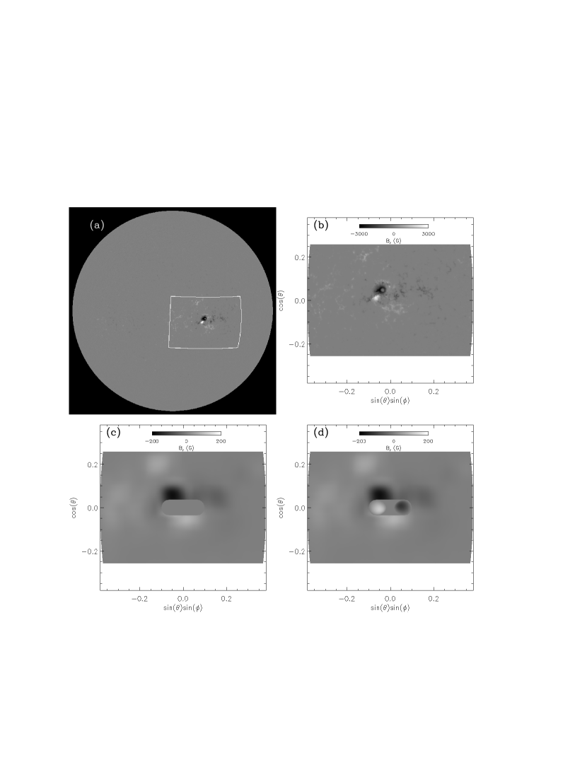
Figure 1: (a) MDI full-disk magnetogram taken at 20:51:01 UT on December 12, 2006. The surface area enclosed by the white box corresponds to the lower boundary surface of the simulation domain. (b) $B_{r}$ on the lower boundary region as viewed straight-on from the center of the region. (c) $B_{r}$ on the lower boundary after applying a Gaussian smoothing and with the field in a central region being zeroed out for imposing the emergence of a twisted magnetic flux rope. The potential field extrapolated from the $B_{r}$ shown here is the assumed initial field in the simulation domain (see Fig. 2 below) . (d) $B_{r}$ on the lower boundary at the end of emergence of the twisted flux rope.

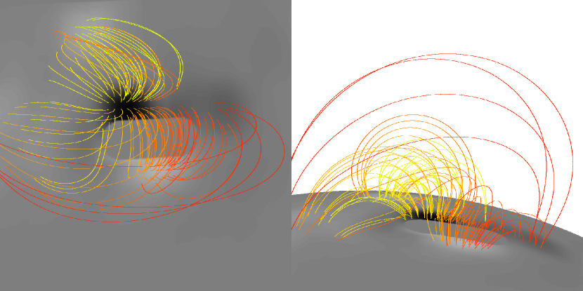
Figure 2: Selected field lines of the initial potential magnetic field for the simulation as viewed from two different perspectives.

The simulation is set up where we drive the emergence of a part of a twisted magnetic torus at the lower boundary into a pre-existing coronal potential field, constructed based on the MDI full-disk magnetogram from 20:51:01 UT on December 12, 2006 (Figure 1a). First, from the full-disk MDI magnetogram, a region centered on the $\delta$-spot (the white box in Figure 1a), with an latitudinal extent of $30^{\circ}$ and a longitudinal extent of $45^{\circ}$ is extracted as the lower boundary of the spherical simulation domain. In terms of the the simulation coordinates, the domain spans $r\in[R_{\odot},6.25R_{\odot}]$, $\theta\in[75^{\circ},105^{\circ}]$, $\phi\in[-22.5^{\circ},22.5^{\circ}]$, with the center of its lower boundary: $\theta=90^{\circ}$ and $\phi=0^{\circ}$, corresponding to the center of the white-boxed area in Figure 1a. This domain is resolved by a grid of $512\times 352\times 528$, with 512 grid points in $r$, 352 grid points in $\theta$, and 528 grid points in $\phi$. The grid is uniform in the $\theta$ and $\phi$ directions but non-uniform in $r$, with a uniform grid spacing of $dr=1.028$ Mm in the range of $r=R_{\odot}$ to about $1.6R_{\odot}$ and a geometrically increasing grid spacing above $1.6R_{\odot}$, reaching about $dr=173.4$ Mm at the outer boundary. We assume perfectly conducting walls for the side boundaries, and for the outer boundary we use a simple outward extrapolating boundary condition that allows plasma and magnetic field to flow through. The lower boundary region extracted from the MDI full disk magnetogram (as viewed straight-on) is shown in Figure 1b, where we simply take the interpolated line-of-sight flux density from the full-disk magnetogram and assume that the magnetic field is normal to the surface to obtain the $B_{r}$ shown in the Figure. The region contains roughly all the flux of the $\delta$-spot and the surrounding pores and plages, to which some of the flux of the $\delta$-spot is connected. The peak field strength in the region is about $3000$ G. A smoothing using a Gaussian filter is carried out on the lower boundary region until the peak field strength is reduced to about $200$ G. This is necessary since the simulation domain corresponds to the corona, with the lower boundary density assumed to be that of the base of the corona, and thus a significant reduction of the field strength from that measured on the photosphere is needed to avoid unreasonably high Alfv́en speeds, which would put too severe a limit on the time step of numerical integration. After the smoothing, the magnetic flux in a central area, which roughly encompasses the region of the observed flux emergence (including the rotating, positive sunspot) is zeroed out (see Figure 1c) to be the area where the emergence of an idealized, twisted magnetic torus is driven on the lower boundary. The potential field constructed from this lower boundary normal flux distribution in Figure 1c is assumed to be the initial coronal magnetic field for our simulation, which is shown in Figure 2. We zero out the normal flux in the area for driving the flux emergence so that we can specify analytically the subsurface emergence structure in a field free region without the complication of the subsurface extension of a pre-existing flux in the same area.

The initial atmosphere in the domain is assumed to be a static polytropic gas:

$$\rho=\rho_{0}\left[1-\left(1-\frac{1}{\gamma}\right)\frac{GM_{\odot}}{R_{\odot}}\frac{\rho_{0}}{p_{0}}\left(1-\frac{R_{\odot}}{r}\right)\right]^{\frac{1}{1-\gamma}}$$ (9)

$$p=p_{0}\left[1-\left(1-\frac{1}{\gamma}\right)\frac{GM_{\odot}}{R_{\odot}}\frac{\rho_{0}}{p_{0}}\left(1-\frac{R_{\odot}}{r}\right)\right]^{\frac{\gamma}{1-\gamma}}$$ (10)

where $\rho_{0}=8.365\times 10^{-16}$ g ${\rm cm}^{-3}$, and $p_{0}=0.152$ dyne ${\rm cm}^{-2}$ are respectively the density and pressure at the lower boundary of the coronal domain, and the corresponding assumed temperature at the lower boundary is 1.1 MK. The initial magnetic field in the domain is potential, and thus does not exert any forcing on the atmosphere which is in hydrostatic equilibrium. Figure 3 shows the height profiles of the Alfvén speed and the sound speed along a vertical line rooted in the peak $B_{r}$ of the main pre-existing negative polarity spot. For the initial state constructed, the peak Alfvén speed is about 24 Mm/s, and the sound speed is 141 km/s at the bottom and gradually declines with height. In most of the simulation domain, the Alfvén speed is significantly greater than the sound speed.

At the lower boundary (at $r=R_{\odot}$), we impose (kinematically) the emergence of a twisted torus ${\bf B}_{\rm tube}$ by specifying a time dependent transverse electric field ${\bf E}_{\perp}|_{r=R_{\odot}}$ that corresponds to the upward advection of the torus with a velocity ${\bf v}_{\rm rise}$:

$${\bf E}_{\perp}|_{r=R_{\odot}}={\hat{\bf r}}\times\left[\left(-\frac{1}{c}\,{\bf v}_{\rm rise}\times{\bf B}_{\rm tube}(R_{\odot},\theta,\phi,t)\right)\times{\hat{\bf r}}\right].$$ (11)

The magnetic field ${\bf B}_{\rm tube}$ used for specifying ${\bf E}_{\perp}|_{r=R_{\odot}}$ is an axisymmetric torus defined in its own local spherical polar coordinate system ($r^{\prime}$, $\theta^{\prime}$, $\phi^{\prime}$) whose polar axis is the symmetric axis of the torus. In the sun-centered simulation spherical coordinate system, the origin of the ($r^{\prime}$, $\theta^{\prime}$, $\phi^{\prime}$) system is located at ${\bf r}={\bf r}_{c}=(r_{c},\theta_{c},\phi_{c})$, and its polar axis (the symmetric axis of the torus) is in the plane of the ${\hat{\bf\theta}}$ and ${\hat{\bf\phi}}$ vectors at position ${\bf r}_{c}$ and tilted from the $-{\hat{\bf\theta}}$ direction clockwise (towards the ${\hat{\bf\phi}}$ direction) by an angle $\delta$. In the ($r^{\prime}$, $\theta^{\prime}$, $\phi^{\prime}$) system,

$${\bf B}_{\rm tube}=\nabla\times\left(\frac{A(r^{\prime},\theta^{\prime})}{r^{\prime}\sin\theta^{\prime}}\hat{\bf\phi^{\prime}}\right)+B_{\phi^{\prime}}(r^{\prime},\theta^{\prime})\hat{\bf\phi^{\prime}},$$ (12)

where

$$A(r^{\prime},\theta^{\prime})=\frac{1}{4}qa^{2}B_{t}\left(1-\frac{\varpi^{2}(r^{\prime},\theta^{\prime})}{a^{2}}\right)^{2},$$ (13)

$$B_{\phi^{\prime}}(r^{\prime},\theta^{\prime})=\frac{aB_{t}}{r^{\prime}\sin\theta^{\prime}}\left(1-\frac{\varpi^{2}(r^{\prime},\theta^{\prime})}{a^{2}}\right).$$ (14)

In the above, $a$ is the minor radius of the torus, $\varpi=(r^{\prime 2}+R^{\prime 2}-2r^{\prime}R^{\prime}\sin\theta^{\prime})^{1/2}$ is the distance to the curved axis of the torus, where $R^{\prime}$ is the major radius of the torus, $q$ denotes the angular amount (in rad) of field line rotation about the axis over a distance $a$ along the axis, and $B_{t}a/R^{\prime}$ gives the field strength at the curved axis of the torus. The magnetic field ${\bf B}_{\rm tube}$ is truncated to zero outside of the flux surface whose distance to the torus axis is $\varpi=a$. We use $a=0.035R_{\odot}$, $R^{\prime}=0.063R_{\odot}$, $q/a=-0.0308$ rad ${\rm Mm}^{-1}$, $B_{t}a/R^{\prime}=111$ G. The torus center is assumed to be initially located at ${\bf r}_{c}=(r_{c}=0.902R_{\odot},\,\theta_{c}=90^{\circ},\,\phi_{c}=0^{\circ})$, and the tilt of the torus $\delta=0$. Thus the torus is initially entirely below the lower boundary and is in the azimuthal plane. For specifying ${\bf E}_{\perp}|_{r=R_{\odot}}$, we assume that the torus moves bodily towards the lower boundary at a velocity ${\bf v}_{\rm rise}=v_{\rm rise}\hat{{\bf r}}_{c}$, where $v_{\rm rise}$ is described later. The imposed velocity field at the lower boundary is a constant ${\bf v}_{\rm rise}$ in the area where the emerging torus intersects the lower boundary and zero in the rest of the area. The resulting normal flux distribution on the lower boundary after the imposed emergence has stopped is shown in Figure 1d. In it an east-west oriented bipolar pair has emerged, where the positive spot represents the emerging, rotating positive sunspot at the south edge of the dominant negative spot in Figure 1b, and the negative spot corresponds to the flux in the fragmented pores and plages to the west of the rotating positive sunspot in Figure 1b. Observational study by Min and Chae (2009) found that the minor, fragmented pores of negative polarity emerged and moved westward while the positive rotating sunspot moved eastward, suggesting that they are the counterpart to which the positive rotating sunspot is at least partly connected to (see Figure 2 in Min and Chae (2009)). This is one of the reasons that we model the coronal magnetic field in this study with the emergence of an east-west oriented twisted flux rope. After the emergence is stopped, the transverse electric field on the lower boundary (eq. [11]) is set to zero and the magnetic field is line-tied at the lower boundary. At the end of the emergence, the peak normal field strength in the emerged bipolar region on the lower boundary reaches 121 G, compared to the 178 G peak normal field strength in the dominant negative pre-existing spot in the initial lower boundary field. Due to the substantial smoothing of the observed normal magnetic flux density, the total unsigned flux on the lower boundary of our simulation is only about 30% of that on the photosphere in the boxed area shown in Figure 1a. However, the ratio of the emerged flux (in the flux rope) over the total flux on the lower boundary, $\sim 10$%, for our simulation is about the same as the ratio of the observed emerged flux (in the positive rotating sunspot) over the total flux in the boxed area in Figure 1a.

Note that although the coronal temperature and density are used at the lower boundary, the dynamic property of the lower boundary reflects the property of the photosphere. The lower boundary is assumed to be “infinitely heavy” such that the magnetic stress exerted on it from the corona does not result in any motion of the field line foot-points (field anchoring or line-tying) and that the lower boundary evolves in a prescribed way by a kinematically imposed flux emergence associated with the upward advection of a twisted flux rope. Thus dynamically the lower boundary is meant to approximate the photosphere, which can support cross-field currents and the resulting magnetic stresses. However the thermodynamic conditions of the corona (instead of the photosphere) are used for the lower boundary so that (1) we do not have to resolve the small (about 150 km) photospheric pressure scale height in a simulation of the large scale coronal evolution of a CME (size scale on the order of a solar radius), and (2) we avoid solving the complex energy transport associated with coronal heating, radiative cooling, and thermal conduction, which would be required if we were to include the thermodynamics of the photosphere-chromosphere-corona system in the simulation. Here for modeling the large scale, magnetically dominated dynamic evolution of the CME initiation, we greatly simplify the thermodynamics (assuming an ideal polytropic gas for the coronal plasma throughout the domain), and focus on the magnetic field evolution of the corona in response to the imposed flux emergence and field-line anchoring representative of the heavy photospheric lower boundary.

In the remainder of the paper, quantities are expressed in the following units unless otherwise specified: $R_{\odot}=6.96\times 10^{10}\,{\rm cm}$, $\rho_{0}=8.365\times 10^{-16}\,{\rm g/cm^{3}}$, $B_{0}=20\,{\rm G}$, $v_{a0}=B_{0}/\sqrt{4\pi\rho_{0}}=1951\,{\rm km/s}$, $\tau_{a0}=R_{\odot}/v_{a0}=356.8\,{\rm s}$, as units for length, density, magnetic field, velocity and time respectively. Due to the large peak Alfvén speed ($\sim 12v_{a0}\sim 24,000$ km/s) in the domain (see Figure 3), we initially drive the emergence of the twisted torus through the lower boundary at a fairly high speed over a period of $t=0$ to $t=1.2$ with $v_{\rm rise}=0.05v_{a0}\sim 98$km/s, which is just under the sound speed at the lower boundary but significantly slower than the Alfvén speed. In this way we build up the pre-eruption coronal magnetic field approximately quasi-statically and yet fast enough to minimize numerical diffusion. After $t=1.2$, we significantly reduce the driving speed of the flux emergence at the lower boundary to $v_{\rm rise}=0.01v_{a0}$ and thus allow the coronal magnetic field to evolve quasi-statically until it erupts dynamically.

3 Results

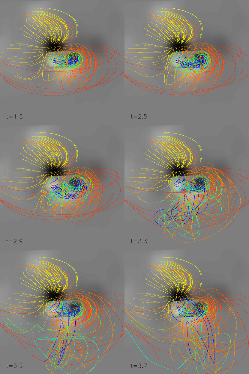
Figure 4: Snapshots of the 3D coronal magnetic field evolution after $t=1.2$ (when the initial fast emergence phase has ended), showing the quasi-static rise and then the eruption of the coronal flux rope. The field is viewed from the observation perspective at the time of the observed flare, where the center of the emerging flux rope is located at $7.1^{\circ}$S and $24^{\circ}$W from the solar disk center (or the line-of-sight). A .gif movie of the above evolution is available in the electronic version of the paper

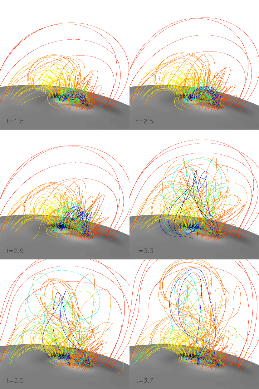
Figure 5: Same as Figure 4 except viewed from a different perspective. A .gif movie of the evolution is available in the electronic version of the paper

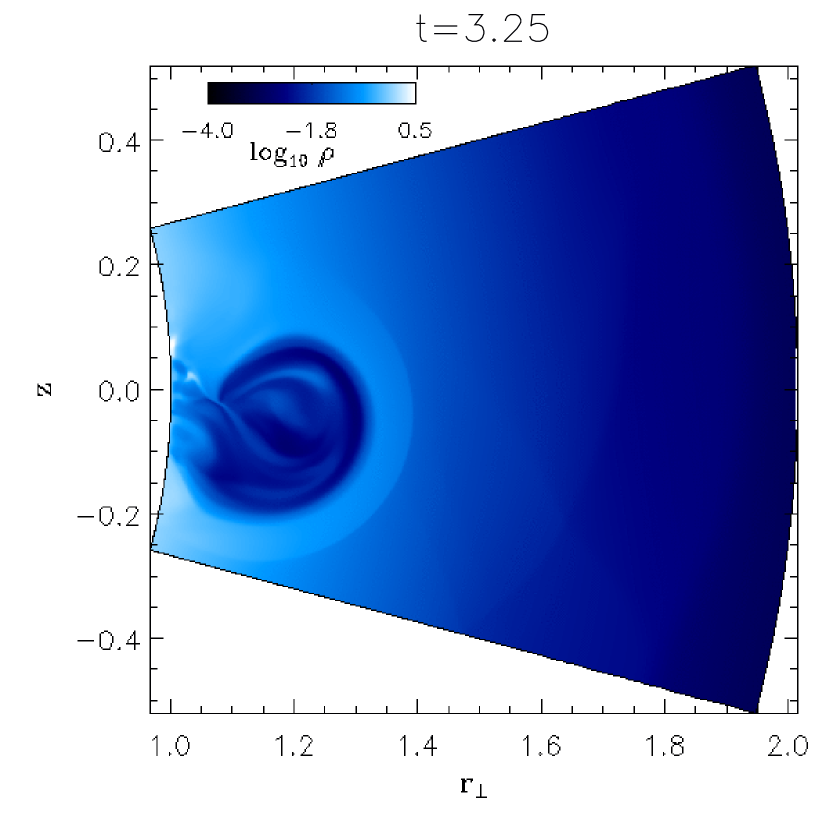
Figure 7: A meridional slice of density through the middle of the erupting flux rope. It shows a low density cavity corresponding to the expanding flux rope. A shock front has formed with a dense sheath compressed between the flux rope and the shock front.

Figures 4 and 5 show snapshots of the 3D coronal magnetic field evolution (as viewed from 2 different perspectives) after the initial stage of relatively fast emergence has ended at $t=1.2$, and the speed for driving the flux emergence at the lower boundary has been reduced to $v_{\rm rise}=0.01v_{a0}$. The view shown in Figure 4 corresponds to the observation perspective at the time of the flare, for which the center of the emerging region (also the center of the simulation lower boundary) is located at $7.1^{\circ}$S and $24^{\circ}$W from the solar disk center (or the line-of-sight). GIF movies for the evolution shown in Figure 4 and Figure 5 are available in the electronic version of the paper. We see that the emerged coronal flux rope settles into a quasi-static rise phase and then undergoes a dynamic eruption. Figure 6 shows the evolution of the rise velocity $v_{r}$ measured at the apex of the tracked axis of the emerged flux rope (triangle points), and also measured at the leading edge of the flux rope (crosses). After the emergence is slowed down at $t=1.2$, the rise velocity at the apex of the flux rope axis slows down, and undergoes some small oscillations as the flux rope settles into a quasi-static rise. The quasi-static rise phase extends from about $t=1.2$ until about $t=2.5$, over a time period of $1.3$, long compared to the dynamic time scale of $\sim 0.1$ for the estimated Alfvén crossing time of the flux rope. At about $t=2.5$, the flux rope axis starts to accelerate significantly and a dynamic eruption ensues. The flux emergence is stopped at $t=2.8$, after which the flux rope continues to accelerate outward. We are able to follow the acceleration of the axial field line up to $v_{r}=0.54=1050$ km/s at $t=3.$, when the axial field line undergoes a reconnection and we are subsequently unable to track it. Figure 6 also shows $v_{r}$ measured at the leading edge of the low density cavity (as shown in Figure 7), corresponding to the expanding flux rope. We find that by the time of about $t=3.2$, a shock front followed by a condensed sheath has formed ahead of the flux rope cavity (see Figure 7 at $t=3.25$), and the $v_{r}$ measured at the front edge of the cavity (or the inner edge of the sheath) reaches a steady speed of about 0.425 or 830 km/s (see crosses in Figure 6).

When the flux rope begins significant acceleration (at $t\approx 2.5$), the decay index $n\equiv d\ln|{\bf B}_{p}|/d\ln h$ which describes the rate of decline of the corresponding potential field ${\bf B}_{p}$ with height $h$ is found to be $n\approx 1.2$ at the apex of the flux rope axis, and $n\approx 1.4$ at the apex of the flux rope cavity. These values are smaller than the critical value of $n_{\rm crit}=1.5$ for the onset of the torus instability for a circular current ring (Bateman, 1978; Kliem and Török, 2006; Demoulin and Aulanier, 2010), although there is a range of variability for the critical value $n_{\rm crit}$, which can be as low as $1$, depending on the shape of the current channel of the flux rope (e.g. Demoulin and Aulanier, 2010). For a 3D anchored flux rope, as is the case here, it is difficult to obtain an analytical determination of $n_{\rm crit}$ for the instability or loss of equilibrium of the flux rope (Isenberg and Forbes, 2007). The exact critical point for the onset of the torus instability would depend on the detailed 3D magnetic field configuration. On the other hand, a substantial amount of twist has been transported into the corona at the onset of eruption. At $t=2.5$, the self-helicity of the emerged flux rope reaches about $-1.02\Phi_{\rm rope}^{2}$, where $\Phi_{\rm rope}$ is the total magnetic flux in the rope, corresponding to field lines in the flux rope winding about the central axis by about 1.02 rotations between the anchored foot points. This suggests the possible development of the helical kink instability of the flux rope (e.g. Hood and Priest, 1981; Török and Kliem, 2005; Fan and Gibson, 2007). The erupting flux rope is found to undergo substantial writhing or kinking motion as can be seen in the sequences of images (also the movies in the electronic version) in Figures 4 and 5.

We also find that the trajectory for the eruption of the flux rope is not radial because of the ambient coronal magnetic field: the erupting flux rope is deflected southward and eastward from the local radial direction (see Figures 4, 5, and 7 and the associated movies). Using the apex location of the erupting flux rope cavity at $t=3.25$ (Figure 7), we find that the erupting trajectory at that time is deflected by $2.3^{\circ}$ southward and $1.3^{\circ}$ eastward from the local radial direction at the center of flux emergence, and further deflection of the trajectory continues with time. Since the local radial direction at the center of the flux emergence corresponds to $7.1^{\circ}$S and $24^{\circ}$W from the solar disk center (or the line-of-sight), the deflection during the eruption is sending the flux rope towards the line-of-sight in the east-west direction, but further southward away from the line-of-sight in the north-south direction. This is consistent with the observed halo of the CME seen in LASCO C2 and C3 coronagraphs (Figure 2 in Kataoka et al. (2009) and Figure 1 in Ravindra and Howard (2010)), where the north-south and east-west asymmetries of the halo distribution indicate that the direction of ejection is more southward and less westward than what would have been expected for a radial ejection from the location of the source region on the solar disk.

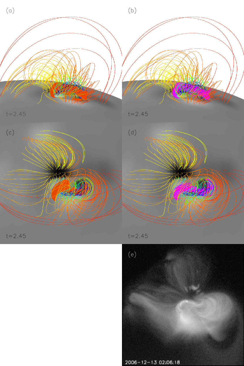
Figure 8: Coronal magnetic field as viewed from the side (a and b) and viewed from the observing perspective (c and d) just before the onset of eruption at $t=2.45$, compared with the Hinode XRT image of the region (e) just before the flare. The orange surfaces are the iso-surfaces where $J/B=1/l$ with $l=$ 10 times the grid size and where $\Delta S/C_{v}>1.15$. They outline the region of strong electric current layers. The purple field lines are the field lines that go through the points in the current layer.

Figure 8 shows the coronal magnetic field as viewed from the side (panels a and b) and viewed from the observing perspective (panels c and d) just before the onset of eruption at $t=2.45$, compared with the Hinode XRT image of the region (panel e) just before the flare. We see that the morphology of the coronal magnetic field and its connectivity are very similar to those shown in the X-ray image. To understand the nature of the bright X-ray sigmoid in the image, we have identified the region of significant magnetic energy dissipation and heating in the simulated magnetic field using both the electric current density $J\equiv|\nabla\times{\bf B}|$ and the increase of entropy $\Delta S=C_{v}\Delta\ln(p/{\rho}^{\gamma})$. As pointed out in Section 2, since we are solving the total energy equation in conservative form, numerical dissipation of magnetic energy and kinetic energy due to the formation of current sheets and other sharp gradients is being implicitly put back into the thermal energy of the plasma, resulting in an increase of the entropy. We have identified regions where there is significant entropy increase with $\Delta S/C_{v}>1.15$ and also high electric current density concentration with $J/B>1/l$ where $l=10$ times the grid size. Such regions are outlined by the orange iso-surfaces in panels (a) and (c) of Figure 8, and they appear as an inverse-S shaped layer (as viewed from the top), which likely corresponds to the formation of an electric current sheet underlying the anchored flux rope (e.g Titov and Demoulin, 1999; Low and Berger, 2003; Gibson et al., 2006). We have also plotted field lines (purple field lines shown in panels b and d) going through the region of the current layer, which are preferentially heated and are expected to brighten throughout their lengths (due to the high heat conduction along the field lines) in soft-X ray, producing the central dominant X-ray sigmoid seen in the Hinode XST image (panel e). Thus our quasi-equilibrium coronal magnetic field resulting from the emergence of a nearly east-west oriented magnetic flux rope could reproduce the observed overall morphology and connectivity of the coronal magnetic field, including the presence of the observed pre-eruption X-ray sigmoid. We find that both $J/B$ as well as $\Delta S$ peak along the “left elbow” portion of the current layer, where the positive polarity flux of the emerged flux rope comes in contact with the flux of the dominant pre-existing negative polarity sunspot, consistent with the brightness distribution along the observed X-ray sigmoid (panel e of Figure 8). Reconnections in this part of the current layer cause some of the flux in the emerged flux rope to become connected with the major negative sunspot (see the green field lines connecting between the dominant negative spot and the emerging positive spot in panel (d) of Figure 8). We have also done a few simulations where we varied the tilt of the emerging flux rope, and found that to reproduce the observed orientation of the sigmoid, the emerging flux rope needs to be nearly east-west oriented.

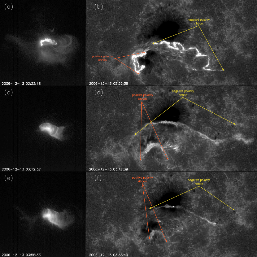
Figure 9: Hinode XRT images of the post-flare brightening (left column images), and the corresponding Hinode SOT snapshots in Ca II line showing the chromosphere flare ribbons (right column images). The orange (yellow) arrows indicate the extent of the flare ribbon in the positive (negative) polarity.

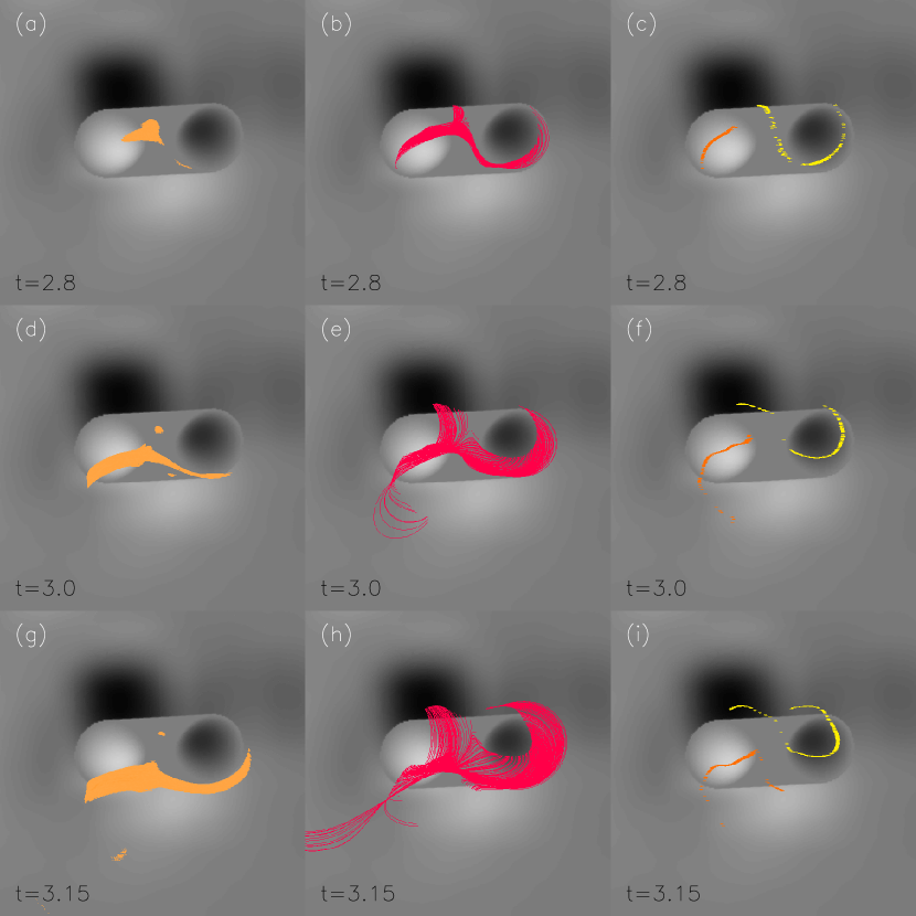
Figure 10: Left column images: iso-surfaces where $J/B=1/l$ with $l=$ 5 times the grid size and where $\Delta S/C_{v}>2.3$, outlining the the most intensely heated portion of the current layer. Middle column images: sampled field lines whose apexes are in the intense current layer outlined by iso-surfaces in the left column images, corresponding to the post-reconnection loops. Right column images: foot points of the post-flare loops shown in the middle column images. The gray scale images in all panels show the normal magnetic field at the lower boundary of the simulation domain

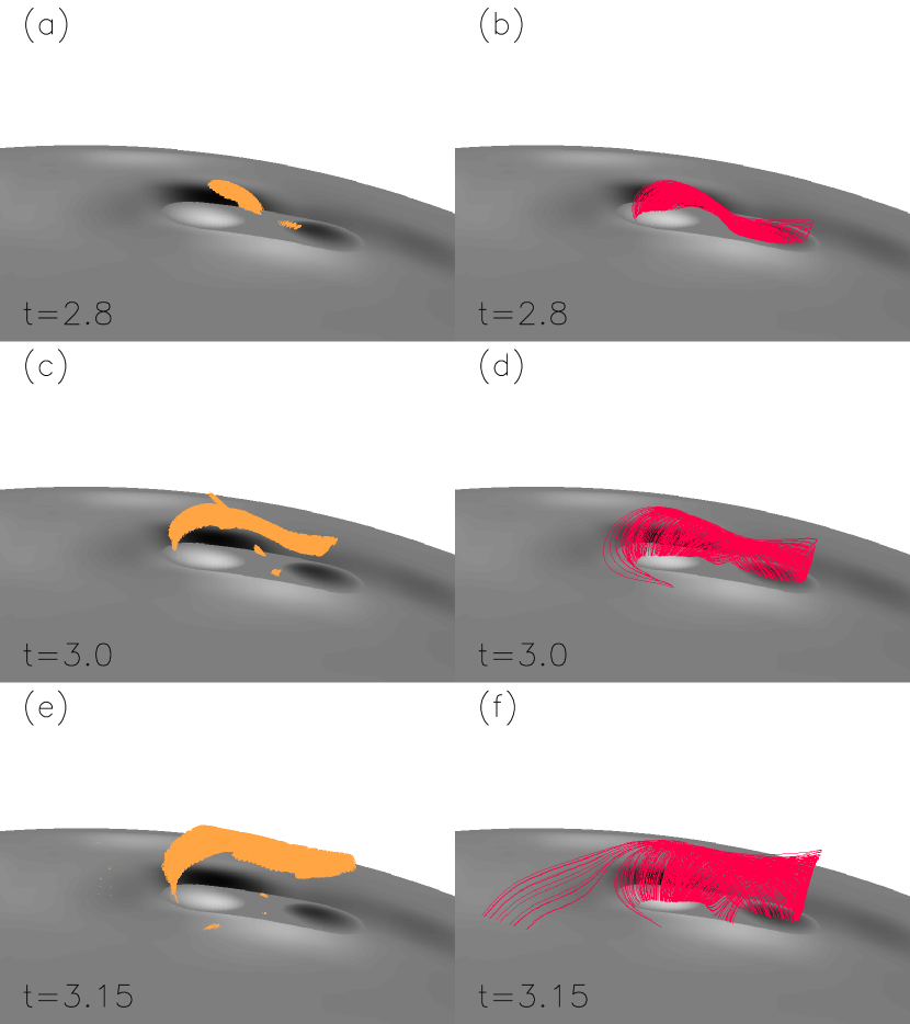
Figure 11: Same as the left and middle columns of Figure 10 but viewed from a different perspective.

With the onset of the eruptive flare, the soft-X ray observation first shows a transient brightening of the sigmoid, and subsequently the emission is completely dominated by the brightness of the post-flare loops (see panels (a)(c)(e) of Figure 9). In the simulated coronal magnetic field, we find that the current density in the inverse-S shaped current layer intensifies as the flux rope begins to erupt. We can deduce qualitatively the evolution of the post-reconnection (or post-flare) loops from our modeled magnetic field evolution. We traced field lines (see the red field lines in panels (b)(e)(h) of Figure 10 and panels (b)(d)(f) of Figure 11) whose apexes are located in the layer of the most intense current density and heating. These field lines are the ones who have just reconnected at their apexes and would slingshot downwards, corresponding to the downward collapsing post-flare loops. The layer of the most intense current density and heating, as outlined by the orange iso-surfaces in panels (a)(d)(g) of Figure 10 and panels (a)(c)(e), is identified as where $J/B>1/l$ with $l=$ 5 times the grid size, and where $\Delta S/C_{v}>2.3$. This most intense current layer is found to rise upward with the eruption of the flux rope. The associated post-reconnection field lines are initially low lying and form a narrow sigmoid shaped bundle as can be seen in Figures 10(b) and 11(b). With time, the post-reconnection loops broaden and rise up, showing cusped apexes (Figures 10(e)(h) and Figures 11(d)(f)). The morphology of the post-reconnection loops, which transition from an initially narrow low-lying sigmoid bundle to a broad, sigmoid-shaped row of loops with cusped apexes is in qualitative agreement with the observed evolution of the post-flare X-ray brightening shown in Figures 9(a)(c)(e).

The foot points of the post-reconnection loops (panels (c)(f)(i) of Figures 10) can be compared qualitatively with the evolution of the flare ribbons in the lower solar atmosphere as shown in the Hinode SOT observation (panels (b)(d)(f) of Figure 9). The ribbon corresponding to the positive polarity foot points (orange ribbon in Figures 10(c)(f)(i)) of the post-reconnection loops is found to sweep southward across the newly emerged positive polarity spot, similar to the apparent movement of the positive polarity ribbon seen the observation (panels (b)(d)(f) of Figure 9) in relation to the observed positive emerging spot. For the ribbon corresponding to the negative polarity footvpoints (the yellow ribbon in Figures 10(c)(f)(i)), its eastern portion is found to extend and sweep northward into the dominant pre-existing negative spot, while its western hook-shaped portion is found to sweep northward across the newly emerged negative spot. Similarly in the SOT observation (panels (b)(d)(f) of Fig 9), for the negative polarity ribbon, the eastern portion sweeps northward into the dominant negative sunspot, while its western, upward curved hook-shaped portion is found to sweep northward across the minor, fragmented negative pores which have emerged to the west of the main $\delta$-sunspot. The modeled ribbons based on the footpoints certainly differ in many ways in their shape and extent compared to the observed flare ribbons. But they capture some key qualitative features in the observed motions of the flare ribbons in relation to the photospheric magnetic flux concentrations.

4 Discussions

We have presented an MHD model that qualitatively describes the coronal magnetic field evolution of the eruptive flare in AR 10930 on December 13, 2006. The model assumes the emergence of an east-west oriented magnetic flux rope into a pre-existing coronal magnetic field constructed based on the MDI full-disk magnetogram of the photospheric magnetic field at 20:51:01 UT on December 12. As described in Section 2, a substantial smoothing of the observed photospheric magnetic flux density from the MDI magnetogram is carried out such that the peak field strength on the lower boundary is reduced from $\sim 3000$ G to $\sim 200$ G to avoid the extremely high Alfvén speed that would put too severe a limit on the time step of numerical integration. The imposed flux emergence at the lower boundary of an idealized subsurface magnetic torus produces a flux emergence pattern on the lower boundary that is only qualitatively representative of the observed flux emergence pattern (compare Figure 1b and Figure 1d). In the model, the emerging bipolar pair on the lower boundary is more symmetric, more spread-out in spatial extent, and both polarities are transporting left-handed twist (or injecting negative helicity flux) into the corona at the same rate. Whereas in the observation, the positive emerging sunspot is coherent and clearly shows a counter-clockwise twisting motion, indicating an injection of negative helicity flux into the corona, while its counterpart to the west is in the form of fragmented pores (e.g. Min and Chae, 2009). However a quantitative measurement by Park et al. (2010) using MDI magnetograms also found a significant negative helicity flux associated with these fragmented pores as well (see Figure 4 in their paper). In the simulation, the self-helicity of the emerged portion of the flux rope in the corona at the end of the imposed flux emergence (at $t=2.8$) is $H_{\rm rope}\approx 1.07\Phi^{2}$, where $\Phi$ is the normal flux in each polarity of the emerged bipolar region on the lower boundary. This is a measure of the internal twist in the emerged flux rope and it corresponds to field lines twisting about the axis by about 1.07 winds (or $385^{\circ}$ rotation) between the two anchored ends in the emerged flux rope. On the other hand, the total relative magnetic helicity $H_{\rm tot}$ that has been transported into the corona by the imposed flux emergence is found to be $H_{\rm tot}\approx 3.02\Phi^{2}$, which is the sum of both the self-helicity of the emerged flux rope $H_{\rm rope}$ as well as the mutual helicity between the emerged flux and the pre-existing coronal magnetic field. The observed amount of rotation of the positive emerging sunspot, ranging from $240^{\circ}$ (Zhang, Li, and Song, 2007) to $540^{\circ}$ (Min and Chae, 2009), gives an estimate of $(H_{\rm rope}/\Phi^{2})\times 360^{\circ}$ for the emerged flux rope, which is about $385^{\circ}$ in the simulation and is thus within the range of the observed values.

After an initial phase where we drive the emergence of the twisted torus at a fairly large (but still significantly sub-Alfvénic) speed to quickly build up the pre-eruption field, we slow down the emergence and the coronal magnetic field settles into a quasi-equilibrium phase, during which the coronal flux rope rises quasi-statically as more twist is being transported slowly into the corona through continued flux emergence. This phase is followed by a dynamic eruption phase where the coronal flux rope accelerates in the dynamic time scale to a steady speed of about 830 km/s. Due to the substantial twist (greater than 1 full wind of field line twist) that has been transported into the corona at the onset of the eruption, the erupting flux rope is found to undergo substantial writhing motion. The erupting flux rope underwent a counter-clockwise rotation that exceeded $90^{\circ}$ by the time the front of the flux rope cavity reached $1.4R_{\odot}$. We also find that the initial trajectory of the erupting flux rope is not radial, but is deflected southward and eastward from the local radial direction due to the ambient coronal magnetic field. Since the initial coronal flux rope is located at $7.1^{\circ}$S and $24^{\circ}$W from the solar disk center, the deflection is sending the erupting flux rope towards the line-of-sight in the east-west direction, but further away from the line-of-sight in the north-south direction, consistent with the observed halo of the CME seen in LASCO C2 and C3 coronagraphs, where the halo’s north-south (east-west) asymmetry appears larger (smaller) than would have been expected from a radial eruption of the flux rope from its location on the solar disk. However, due to the relatively restrictive domain width in $\theta$ ($30^{\circ}$) and $\phi$ ($45^{\circ}$) in our current simulation, the side wall boundary in the south begins to significantly constrain the further southward deflection and expansion of the flux rope by the time the top of the flux rope cavity reaches about $1.4R_{\odot}$. Thus, we are not able to accurately determine the subsequent trajectory change or the continued writhing of the erupting flux rope beyond this point. A larger simulation with a significantly greater domain size in $\theta$ and $\phi$, that still adequately resolves the coronal magnetic field in the source region, will be carried out in a subsequent study to determine the later properties of the flux rope ejecta.

The restrictive domain size may also play a role in the significantly lower steady speed of $830$ km/s reached by the erupting flux rope in the simulation, compared to the observed value of at least $1780$ km/s for the speed of the CME (e.g. Ravindra and Howard, 2010). It has been shown that the rate of spatial decline of the ambient potential magnetic field with height is both a critical condition for the onset of the torus instability of the coronal flux rope (Bateman, 1978; Kliem and Török, 2006; Isenberg and Forbes, 2007; Fan, 2010; Demoulin and Aulanier, 2010, e.g.) as well as an important factor in determining the acceleration and the final speed of the CMEs (Török and Kliem, 2007). Even for a sufficiently twisted coronal flux rope that is unstable to the helical kink instability, the spatial decline rate of the ambient potential field is found to determine whether the non-linear evolution of the kink instability leads to a confined eruption (with the flux rope settles into a new kinked equilibrium) or an ejection of the flux rope (Török and Kliem, 2005). The simulation in this paper has assumed perfect conducting walls for the side boundaries where the field lines are parallel to the walls. Thus widening the simulation domain would result in a more rapid expansion and hence a more steep decline of the ambient potential field with height. This would result in a greater acceleration and a faster final speed for the CME based on the results from previous investigations by Török and Kliem (2005, 2007). It may be difficult to distinguish whether the torus or the kink instability initially triggers the eruption given the complex 3D coronal magnetic field, but the final speed of the CME would be strongly affected by the spatial decline rate of the ambient potential field for either cases. The substantial smoothing of the lower boundary magnetic field to reduce the peak Alfvén speed is also a major reason for the low final speed of the erupting flux rope in the current simulation.

Nevertheless, our simulated coronal magnetic field evolution is found to reproduce several key features of the eruptive flare observed by Hinode. The pre-eruption coronal field during the quasi-static phase reproduces the observed overall morphology and connectivity of the coronal magnetic field, including the presence of the pre-eruption X-ray sigmoid seen in the Hinode XRT images. The presence of the pre-eruption sigmoid in our model is caused by the preferential heating of an inverse-S shaped flux bundle in the flux rope by the formation of an inverse-S shaped current sheet underlying the flux rope. Our simulations suggest that the emerging flux rope needs to be nearly east-west oriented in order to reproduce the observed orientation of the X-ray sigmoid. This is consistent with the suggestion by (Min and Chae, 2009) that the counterpart of the emerging, rotating positive sunspot is the minor negative pores to the west of the emerging sunspot (rather than the dominant negative sunspot). After the onset of the eruption, the morphology of the post-flare loops deduced from the simulated field show a transition from an initial narrow, low-lying sigmoid bundle to a broad, sigmoid-shaped row of loops with cusped apexes, in qualitative agreement with the evolution of the post-flare X-ray brightening observed by XRT of Hinode. The apparent motions of the foot points of the post-flare loops in relation to the lower boundary magnetic flux concentrations are also in qualitative agreement with the evolution of the chromospheric flare ribbons observed by Hinode SOT. These agreements suggest that our simulated coronal magnetic field produced by the emergence of an east-west oriented twisted flux rope, with the positive emerging flux “butting against” the southern edge of the dominant pre-existing negative sunspot, captures the gross structure of the actual magnetic field evolution associated with the eruptive flare. To improve quantitative agreement, a more accurate determination of the lower boundary electric field (Fisher et al., 2011) that more closely reproduces the observed flux emergence pattern on the lower boundary is needed.

Figure 3: The Alfvén speed and the sound speed as a function of raidial distance along a vertical line rooted in the peak $B_{r}$ of the main pre-existing negative spot on the lower boundary

Figure 6: The evolution of the radial velocity measured at the apex of the tracked axial field line of the emerged flux rope (triangles) and also measured at the leading edge of the flux rope cavity (crosses).

References

- Amari et al. (2000) Amari, T., Luciani, J. F., Mikic, Z., Linker, J., 2000, ApJ., 529, L49
- Antiochos et al. (1999) Antiochos, S. K. and DeVore, C. R. and Klimchuk, J. A. 1999, ApJ, 510, 485.
- Aulanier et al. (2010) Aulanier, G., Török, T., Demoulin, P., and DeLuca, E. 2010, ApJ, 708, 314.
- Bateman (1978) Bateman, G., MHD Instabilities, 1978, MIT Press, Cambridge, MA, and London, England, p. 84-85
- Chen (2011) Chen, P. F. 2011, Living Rev. Solar Phys., 8, (2011), 1. URL (cited on May 2011): http://www.livingreviews.org/lrsp-2011-1
- Demoulin and Aulanier (2010) Démoulin, P., and Aulanier, G. 2010, ApJ, 718, 1388
- Fan (2010) Fan, Y., 2010, ApJ, 719, 728
- Fan and Gibson (2007) Fan, Y., & Gibson, S. E., 2007, ApJ, 668, 1232
- Fisher et al. (2011) Fisher, G., Welsch, B. T., and Abbett, W. P. 2011, Sol. Phys., in press
- Forbes and Priest (1995) Forbes, T. G., and Priest, E. R., 1995, ApJ, 446, 377
- Forbes et al. (2006) Forbes, T. G., and 14 other authors, 2006, Space Sciences Reviews, 123, 251
- Gibson et al. (2006) Gibson, S. E. and Fan, Y. and Török, T. and Kliem, B., 2006, Space Science Reviews, 124, 131
- Hood and Priest (1981) Hood, A. W., & Priest, E. R. 1981, GAFD, 17, 297
- Hundhausen (1993) Hundhausen, A. J., 1993, J. Geophys. Res., 98, 13177
- Inoue et al. (2008) Inoue, S. Kusano, K., Masuda, S., Miyoshi, T., Yamamoto, T., Magara, T., Tsuneta, T., Sakurai, T., Yokoyama, T., and US/Japan SOT team, 2008, ASP conference series, 397, 110
- Isenberg and Forbes (2007) Isenberg, Philip A., and Forbes, Terry G. 2007, ApJ, 670, 1453
- Kataoka et al. (2009) Kataoka, R., Ebisuzaki, T., Kusano, K., Shiota, D., Inoue, S., Yamamoto, T. T., and Tokumaru, M. 2009, J. Geophys. Res., 114, A10102
- Kliem and Török (2006) Kliem, B., and Török, T. 2006, Phys. Rev. Lett., 96, 255002
- Lin et al. (1998) Lin, J, Forbes, T. G., Isenberg, P. A., and Demoulin, P. 1998, ApJ, 504, 1006
- Lindsay et al. (1999) Lindsay, G. M., Luhmann, J. G., Russell, C. T., and Gosling, J. T. 1999, J. Geophys. Res., 104, 12515
- Liu et al. (2008) Liu, Y., Luhmann, J. G., Müller-Mellin, Schroeder, P. C., Wang, L., Lin, R. P., Bale, S. D., Li, Y., Acuna, M. H., and Sauvaud, J.-A. 2008, ApJ, 689, 563.
- Low and Berger (2003) Low, B. C., & Berger, M. 2003, ApJ, 589, 644
- Mikić and Linker (1994) Mikić Zoran and Linker, Jon A. 1994, ApJ, 430, 898
- Mikić et al. (2008) Mikić, Z. and Linker, J. A. and Lionello, R. and Riley, P. and Titov, V. and Odstrcil, D., 2008, AGU spring meeting presentation
- Min and Chae (2009) Min., Soonyoung, and Chae, Jongchul 2009, Sol. Phys., 258, 203
- Park et al. (2010) Park, Sung-Hong, Chae, J., Ju, J., Tan, C., and Wang, H. 2010, ApJ, 720, 1102
- Ravindra and Howard (2010) Ravindra, B., and Howard, T. A. 2010, Bull. Astr. Soc. India, 38, 147
- Rempel, Schüssler, and Knölker (2009) Rempel, M, Schüssler, M., and Knölker, M., 2009, ApJ, 691, 640
- Roussev et al. (2003) Roussev, I. I., Forbes, T. G., Gombosi, T. I., Sokolov, I. V., DeZeeuw, D. L., and Birn, J. 2003, ApJ, 588, L45
- Schrijver et al. (2008) Schrijver, C. J. and De Rosa, M. L. and Metcalf, T. and Barnes, G. and Lites, B. and Tarbell, T. and McTiernan, J. and Valori, G. and Wiegelmann, T. and Wheatland, M. S. and Amari, T. and Aulanier, G. and Démoulin, P. and Fuhrmann, M. and Kusano, K. and Régnier, S. and Thalmann, J. K., 2008, ApJ, 675, 1637
- Stone and Norman (1992a) Stone, J.M., and Norman M.L., 1992, ApJS, 80, 753
- Stone and Norman (1992b) Stone, J.M., and Norman M.L., 1992, ApJS, 80, 791
- Sturrock et al. (2001) Sturrock, P. A., Weber, M., Wheatland, M. S., and Wolfson, R., 2001, ApJ, 548, 492
- Titov and Demoulin (1999) Titov, V. S., and Demoulin P., 1999, A&A, 351, 707
- Titov et al. (2008) Titov, V. S. and Mikic, Z. and Linker, J. A. and Lionello, R., 2008, ApJ, 675, 1614
- Török and Kliem (2005) Török T. & Kliem B. 2005, ApJ, 630, L97
- Török and Kliem (2007) Török T. & Kliem B. 2007, Astron. Nachr., 328, 743
- Webb et al. (2000) Webb, D. F., Cliver, E. W., Crooker, N. U., St. Cyr, O. C., and Thompson, B. J., 2000, J. Geophys. Res., 105, 7491
- Zhang, Li, and Song (2007) Zhang, J., Li, L., Song, Q. 2007, ApJ, 662, L35