Mechanism for enhanced disordered screening in strongly correlated metals: local vs. nonlocal effects

Abstract

We study the low temperature transport characteristics of a disordered metal in the presence of electron-electron interactions. We compare Hartree-Fock and dynamical mean field theory (DMFT) calculations to investigate the scattering processes of quasiparticles off the screened disorder potential and show that both the local and non-local (coming from long-ranged Friedel oscillations) contributions to the renormalized disorder potential are suppressed in strongly renormalized Fermi liquids. Our results provide one more example of the power of DMFT to include higher order terms left out by weak-coupling theories.

1 Introduction

Transport in dirty metals has been investigated for many years, with a substantial theoretical and experimental understanding being achieved in the case of weak disorder and moderate electron-electron interaction lee_ramakrishnan ; punnose05 . However, much less is known about situations with strong electronic correlations, where much of our understanding relies on the application of numerical methods like quantum Monte Carlo scalettar03 or exact diagonalization scalettar08 , which are nevertheless severely limited in temperature range and system sizes. A more flexible approach to investigate the interplay of strong correlations and disorder is provided by the dynamical mean field theory (DMFT) dmft_rmp96 . In its original formulation, the DMFT treatment of disordered systems does not include Anderson localization effects screening_2003 , a limitation which was quickly resolved by the introduction of the statistical DMFT (statDMFT) statdmft ; NFL_2005 . The statDMFT approach has already led to some novel effects like a strong disorder screening by interactions screening_2003 ; proceeding_sces08 , energy-resolved spatial inhomogeneities proceeding_sces08 , and the emergence of an Electronic Griffiths phase in the vicinity of the disordered Mott transition egp01 ; griffiths2d09 .

To partially elucidate the mechanism behind the rich physics uncovered through the statDMFT method, a recent work ripples10 provided analytical insights into the scattering off a weak random disorder potential in an otherwise uniform strongly interacting paramagnetic metal. While the analysis is most straightforward and transparent in this regime, this general issue is of key relevance also for the diffusive regime. Here, we revisit this problem, explicitly comparing the statDMFT results with those of the Hartree-Fock (HF) approximation. Our analytical results highlight the non-perturbative nature of the statDMFT and show that processes left out by HF generate vertex corrections to the impurity potential, which ultimately lead to enhanced screening screening_2003 .

2 Model and methods

We study the paramagnetic phase of the disordered Hubbard model

$$\mathcal{H} = \sum_{i\sigma}\varepsilon_{i}n_{i\sigma}-\sum_{\left\langle ij\right\rangle,\sigma}t_{ij}c_{i\sigma}^{\dagger}c_{j\sigma}+U\sum_{i}n_{i\uparrow}n_{i\downarrow},$$ (1)

where $t_{ij}$ are the hopping matrix elements between nearest-neighbor sites, $c_{i\sigma}^{\dagger}$$\left(c_{i\sigma}\right)$ is the creation (annihilation) operator of an electron with spin projection $\sigma$ at site $i$, $U$ is the on-site Hubbard repulsion, $n_{i\sigma}=c_{i\sigma}^{\dagger}c_{i\sigma}$ is the number operator, and $\varepsilon_{i}$ are the site energies (bare disorder potential). We consider here its paramagnetic phase at half-filling (chemical potential $\mu=U/2$) and a particle-hole symmetric lattice. Below we discuss two different routes to treat this model.

2.1 Hartree-Fock (HF)

To solve the model (1), we first consider the HF approach, as described, for example, in Refs. herbut01 ; nandini04 . Here, we simply decouple the interaction term in (1) as $n_{i\uparrow}n_{i\downarrow}\approx\left\langle n_{i\uparrow}\right\rangle n_{i\downarrow}+n_{i\uparrow}\left\langle n_{i\downarrow}\right\rangle-\left\langle n_{i\uparrow}\right\rangle\left\langle n_{i\downarrow}\right\rangle$. We restrict ourselves to the paramagnetic solution, $\left\langle n_{i\uparrow}\right\rangle=\left\langle n_{i\downarrow}\right\rangle=\left\langle n_{i}\right\rangle$, and the self-consistency condition is obtained from

$$\left\langle n_{i}\right\rangle=T\sum_{\omega_{n}}G_{ii}\left(\omega_{n}\right) = T\sum_{\omega_{n}}\left[\frac{1}{i\omega_{n}\mathbf{1}-\mathbf{v}-\mathcal{H}_{0}}\right]_{ii},$$ (2)

where $T$ is the temperature, $G_{ii}\left(\omega_{n}\right)$ is the local part of the lattice Green’s function, $\omega_{n}$ are the Matsubara frequencies, $\mathcal{H}_{0}$ is the clean ($\varepsilon_{i}=0$) and non-interacting ($U=0$) lattice Hamiltonian, $\mathbf{v}$ is a site-diagonal matrix $\left[\mathbf{v}\right]_{ij}=v_{i}\delta_{ij}$, whose entries

$$v_{i}=\varepsilon_{i}+\Sigma_{i}\left(0\right)-\mu = \varepsilon_{i}+U\left\langle n_{i}\right\rangle-\mu$$ (3)

are the renormalized HF disorder potential, and $\Sigma_{i}\left(0\right)=\Sigma_{i}\left(\omega\right)=U\left\langle n_{i}\right\rangle$ is the frequency-independent HF electronic self-energy. We note that the HF approximation can be regarded as the static (weak-coupling) limit of the statDMFT and that it already contains one of its most important features: a self-energy which is local, but which varies from site to site reflecting spatial disorder fluctuations. As we will show later, the statDMFT contains all the HF diagrams, but it also re-sums many higher order terms left out by HF.

In general, we have to solve the self-consistency equation in (2) numerically. However, for a weak disorder potential ($\left|\varepsilon_{i}\right|\ll D$, where $D$ is the bare half band width), we can expand it around the uniform solution, and, to leading order in the disorder potential, we have

$$v\left(\vec{q}\right) = \frac{\varepsilon\left(\vec{q}\right)}{1-U\Pi_{\vec{q}}}+\mathcal{O}\left[\varepsilon\left(\vec{q}\right)^{2}\right],$$ (4)

where $\varepsilon\left(\vec{q}\right)$ is the inverse lattice Fourier transform of the disorder potential $\varepsilon_{i}$. $\Pi_{\vec{q}}$ is the usual static Lindhard polarization function Mahan_many_body .

As $U\rightarrow 0$, the renormalized disorder potential reads $v_{i}\simeq\varepsilon_{i}+U\Pi_{ij}\varepsilon_{j}$, where $\Pi_{ij}$ is the lattice Fourier transform of $\Pi_{\vec{q}}$, showing that the electrons scatter not only off the bare impurities, but also off the long-ranged potential generated by the Friedel oscillations (encoded in $\Pi_{ij}$). This result contains another general feature of the statDMFT: the renormalized disorder potential acquires non-local terms, which are absent in the original DMFT formulation screening_2003 .

We can easily interpret (4) in terms of the usual diagrammatic perturbation theory if we rewrite it as

$$\frac{v\left(\vec{q}\right)}{\varepsilon\left(\vec{q}\right)} = \frac{1}{\kappa_{RPA}(\vec{q})}=1+U_{eff}^{HF}\left(\vec{q}\right)\Pi_{\vec{q}},$$ (5)

$$U_{eff}^{HF}\left(\vec{q}\right) = \frac{U}{1-U\Pi_{\vec{q}}}=\frac{U}{\kappa_{RPA}(\vec{q})},$$ (6)

where we have defined the dielectric function

$$\kappa_{RPA}(\vec{q})=1-U\Pi_{\vec{q}},$$ (7)

which in this approximation is given by the RPA expression Mahan_many_body . It is then clear that the HF approximation dresses the electron-impurity vertex by a “chain of bubbles”, as in the standard RPA screening theory Mahan_many_body , Fig. (1b).

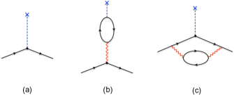
Figure 1: Diagrammatic representation of the electron-impurity interaction: (a) the bare electron-impurity interaction vertex; (b) the first term of the Hartree-Fock theory, which is equivalent to the RPA resummation of “bubbles”; (c) the first vertex correction to the electron-impurity interaction, absent in Hartree-Fock theory, but included in the statDMFT/slave boson solution. The inclusion of these and higher-order vertex corrections is essential for the phenomenon of perfect disorder screening. Here, the wavy line corresponds to the local on-site Hubbard-type electron-electron interaction.

2.2 Slave-bosons (SB)

To investigate the strongly correlated regime, we implement the statDMFT using the slave-boson (SB) mean-field theory of Kotliar and Ruckenstein kotliar_ruckenstein (which is equivalent to the Gutzwiller variational approximation brinkman_rice ) as impurity solver proceeding_sces08 ; griffiths2d09 . This theory is mathematically equivalent to applying directly the original formulation of Kotliar and Ruckenstein to the Hubbard model in (1), as discussed in Ref. proceeding_sces08 .

As in the previous HF calculation, we consider a weak disorder potential and expand the relevant mean-field equations proceeding_sces08 ; griffiths2d09 around their uniform solution. For particle-hole symmetry $Z_{i}=Z_{0}+\emph{O}\left(\varepsilon_{i}^{2}\right)$ and we have, at $T=0$ ripples10

$$v\left(\vec{q}\right) = \frac{\varepsilon\left(\vec{q}\right)}{1-u^{2}-\tilde{U}\Pi_{\vec{q}}}+\mathcal{O}\left[\varepsilon\left(\vec{q}\right)^{2}\right],$$ (8)

where $u=U/U_{c}$ and

$$\tilde{U}=\left(\frac{u}{2}-\frac{1}{1-u}\right)U.$$ (9)

Eq. (8) implies the following dielectric function

$$\kappa_{SB}(\vec{q}) = 1-u^{2}-\tilde{U}\Pi_{\vec{q}}.$$ (10)

The relation $n\left(\vec{q}\right)=1/2+\Pi_{\vec{q}}v\left(\vec{q}\right)$ also holds, as expected. It is instructive to consider the limits of weak and strong interactions. If $U\ll U_{c}$,

$$\kappa_{SB}(\vec{q})\approx 1-U\Pi_{\vec{q}}=\kappa_{RPA}(\vec{q}),$$ (11)

and we recover the HF result. In contrast, as $U\to U_{c}$,

$$\kappa_{SB}(\vec{q})\to-\frac{U_{c}}{1-u}\Pi_{\vec{q}},$$ (12)

leading to

$$v_{i}\simeq-\left(1-U/U_{c}\right)U_{c}^{-1}\left[\mbox{\boldmath$\Pi$}^{-1}\right]_{ij}\varepsilon_{j}.$$ (13)

As the system approaches the Mott transition, the renormalized disorder potential goes to zero at all lattice sites, a situation that was dubbed “perfect disorder screening” in Ref. screening_2003 . Its spatial structure is also very interesting, since $v_{i}$ is just as non-local as for small $U$, but the non-local term is governed not by the Lindhard function, but by its inverse. The spatial structure of the charge disturbance in this limit is given by

$$\delta n_{i}=\left[\left(1-U/U_{c}\right)/U_{c}\right]\varepsilon_{i}+\mathcal{O}\left(\left(1-U/U_{c}\right)^{3}\right).$$ (14)

Thus, although the charge fluctuations are suppressed everywhere, its non-local part, coming from the Friedel oscillations, is much more strongly suppressed ($\mathcal{O}\left(1-u\right)^{3}$) and the electronic density is significantly disturbed only in the immediate vicinity of the impurities. The suppression of the slow spatial decay in $\delta n_{i}$ reflects the fundamental tendency of quasiparticles to become localized as the system approaches the Mott insulator. Therefore, density fluctuations are healed very effectively in the strongly correlated limit.

Additional insight into these results can be obtained by noting that the second term on the right-hand side of Eq. (10) is unimportant both in the weakly and in the strongly correlated limits, cf. Eqs. (11) and (12). Neglecting this term in (10), we can follow the same procedure as in (5) and rewrite (8) as

$$\frac{v\left(\vec{q}\right)}{\varepsilon\left(\vec{q}\right)} = 1+U_{eff}^{SB}\left(\vec{q}\right)\Pi_{\vec{q}},$$ (15)

$$U_{eff}^{SB}\left(\vec{q}\right) = \frac{\tilde{U}}{1-\tilde{U}\Pi_{\vec{q}}}.$$ (16)

The approach to Mott localization in this language can thus be described by the replacement $U\to\tilde{U}$, cf. Eqs. (5) and (6). This replacement, in turn, may be viewed as a local field correction coming from vertex corrections in the polarization function Mahan_many_body ; loc_field05 (see Fig. (1c) and the discussion in Section 3 below). Close to the Mott transition $\tilde{U}\approx U/(1-u)$ diverges and this strong correlation effect is seen to fall completely outside the scope of the HF theory. In fact, whereas HF predicts a gradual decrease of the dielectric function with increasing $U$, signaling the suppressed screening, see Eq. (7), the statDMFT/SB approach predicts precisely the opposite: the dielectric function diverges as $U\to U_{c}$, see Eq. (12), and the screening becomes asymptotically perfect.

3 Beyond weak-coupling

Comparing the renormalized disorder potential in (4) and (8), we see that the interaction corrections left out by HF generate vertex corrections to the impurity potential, which are contained in the effective interaction $U_{eff}^{SB}(\vec{q})$ in (16). Since the HF approximation is the first term in expanding the electronic self-energy in $U$, we expand our solutions (4) and (8) in powers of $U$, in order to track down which terms are left out of HF. As we have seen, to first order in $U$, the statDMFT/SB and HF solutions agree. At second order, a difference emerges already

$$\frac{v_{HF}^{\left(2\right)}\left(\vec{q}\right)}{\varepsilon\left(\vec{q}\right)} = U^{2}\Pi_{\vec{q}}^{2},$$ (17)

$$\frac{v_{SB}^{\left(2\right)}\left(\vec{q}\right)}{\varepsilon\left(\vec{q}\right)} = U^{2}\Pi_{\vec{q}}^{2}+\left(\frac{U}{U_{c}}\right)^{2}\left(1+\frac{3}{2}U_{c}\Pi_{\vec{q}}\right).$$ (18)

To gain insight into the leading correction beyond HF, we combine the statDMFT procedure with usual perturbation theory. First, we recall that in the statDMFT approach the electronic self-energy is local, albeit site-dependent. The only contribution to a local self-energy which is of second order in the interactions is given by mueller-hartmann

$$\Sigma_{i}^{\left(2\right)}\left(i\omega_{n}\right) = U^{2}T\sum_{\nu_{n}}G_{ii}^{\left(0\right)}\left(i\omega_{n}+i\nu_{n}\right)\Pi_{ii}^{\left(0\right)}\left(i\nu_{n}\right),$$ (19)

where

$$\Pi_{ii}\left(i\nu_{n}\right) = T\sum_{\nu^{\prime}_{n}}G_{ii}^{\left(0\right)}\left(i\nu^{\prime}_{n}\right)G_{ii}^{\left(0\right)}\left(i\nu^{\prime}_{n}-i\nu_{n}\right)$$ (20)

is the local contribution of the dynamical Lindhard polarization, calculated using the local Green’s function $G_{ii}^{\left(0\right)}\left(i\omega_{n}\right)=\left[\left(i\omega_{n}-\mbox{\boldmath$\varepsilon$}-\mathcal{H}_{0}\right)^{-1}\right]_{ii}$ with $\mbox{\boldmath$\varepsilon$}_{ij}=\varepsilon_{i}\delta_{ij}$. We are interested only in the leading $\omega_{n}$ behavior of (19), since our statDMFT/SB approach is itself a low-energy one vollhardt_he3 . Ultimately, this low-energy approximation provides a local Fermi-liquid description of the auxiliary impurity problem Hewson_kondo . For example, the uniform contribution $\left(\varepsilon_{i}=0\right)$ of (19) is $\Sigma_{0}^{\left(2\right)}\left(i\omega_{n}\right)\approx$$\left(1-1/Z_{0}^{\left(2\right)}\right)i\omega_{n}+\mathcal{O}\left(\omega_{n}^{2}\right)$, with $\left(1-1/Z_{0}^{\left(2\right)}\right)\propto-U^{2}$, for a particle-hole symmetric lattice.

We now expand (19) and (20) to linear order in the impurity potential. There are three identical contributions, each with one of the three Green’s function lines with an impurity vertex inserted in it, as shown in Fig (1c). We focus on $\Sigma_{i}^{\left(2\right)}\left(0\right)$ since this defines the renormalized disorder potential. Qualitatively, it is very easy to see how the extra terms in (18) are generated. Consider, for simplicity, that we estimate $\Pi_{ii}\left(i\nu_{n}\right)$ in (19) through the clean and static limit $\Pi_{ii}\left(i\nu_{n}\right)\approx\Pi_{0}\left(0\right)=-\rho\left(0\right)\approx-U_{c}^{-1}$. In this case, we simply have $\Sigma_{i}^{\left(2\right)}\left(0\right)\approx\left(U/U_{c}\right)^{2}U_{c}\Pi_{ij}\varepsilon_{j},$ which has the same structure as the last term in (18). Based on these arguments, we stress that the difference which exists already at order $U^{2}$ between (17) and (18) is an interaction-generated vertex correction of the electron-impurity vertex, which is absent in HF/RPA screening theory, but which is re-summed to all orders within statDMFT/SB.

4 Conclusions

We presented a detailed analytical calculation of the effects of weak disorder scattering in a correlated host. Comparing the results obtained within HF and statDMFT, we highlighted the fact that statDMFT incorporates important vertex corrections to all orders, a task which is difficult, or more likely, even impossible to perform using weak-coupling diagrammatic approaches. A physical consequence of the inclusion of these vertex corrections is the phenomenon of disorder screening by interactions.

An analogous example of this dichotomy can be observed in the familiar Migdal-Eliashberg (ME) strong coupling theory describing the electron-phonon problem Mahan_many_body . Indeed, the ME theory neglects the momentum dependence of the electronic self-energy and may thus be regarded as a weak-coupling approximation to DMFT. Like the HF/RPA screening described above, it also neglects vertex corrections. The full DMFT solution, however, not only contains all the ME diagrams, but it also re-sums many higher order terms left out by the ME approach, including vertex corrections hewson02prl , in close analogy with the statDMFT treatment of disorder and interactions. In both models, these strong coupling effects reflect non-perturbative Kondo-like processes screening_2003 ; hewson02prl , which cannot be described by weak-coupling approaches.

- (1) P.A. Lee, T.V. Ramakrishnan, Rev. Mod. Phys. 57, 287 (1985)
- (2) A. Punnoose, A.M. Finkel’stein, Science 310, 289 (2005)
- (3) P.J.H. Denteneer, R.T. Scalettar, N. Trivedi, Phys. Rev. Lett. 83, 4610 (1999)
- (4) S. Chiesa, P.B. Chakraborty, W.E. Pickett, R.T. Scalettar, Phys. Rev. Lett. 101, 086401 (2008)
- (5) A. Georges, G. Kotliar, W. Krauth, M.J. Rozenberg, Rev. Mod. Phys. 68, 13 (1996)
- (6) D. Tanasković, V. Dobrosavljević, E. Abrahams, G. Kotliar, Phys. Rev. Lett. 91, 066603 (2003)
- (7) V. Dobrosavljević, G. Kotliar, Phys. Rev. Lett. 78, 3943 (1997)
- (8) E. Miranda, V. Dobrosavljević, Rep. Prog. Phys. 68, 2337 (2005)
- (9) E.C. Andrade, E. Miranda, V. Dobrosavljević, Physica B 404, 3167 (2009)
- (10) E. Miranda, V. Dobrosavljević, Phys. Rev. Lett. 86, 264 (2001)
- (11) E.C. Andrade, E. Miranda, V. Dobrosavljević, Phys. Rev. Lett. 102, 206403 (2009)
- (12) E.C. Andrade, E. Miranda, V. Dobrosavljević, Phys. Rev. Lett. 104, 236401 (2010)
- (13) I.F. Herbut, Phys. Rev. B 63, 113102 (2001)
- (14) D. Heidarian, N. Trivedi, Phys. Rev. Lett. 93, 126401 (2004)
- (15) G.D. Mahan, Many-Particle Physics (Plenum, New York, 2000), 3rd edn.
- (16) G. Kotliar, A.E. Ruckenstein, Phys. Rev. Lett. 57, 1362 (1986)
- (17) W.F. Brinkman, T.M. Rice, Phys. Rev. B 2, 4302 (1970)
- (18) G.E. Simion, G.F. Giuliani, Phys. Rev. B 72, 045127 (2005)
- (19) E. Müller-Hartmann, Z. Phys. B 76, 211 (1989)
- (20) D. Vollhardt, Rev. Mod. Phys. 56, 99 (1984)
- (21) A.C. Hewson, The Kondo Problem to Heavy Fermions, 1st edn. (Cambridge University Press, Cambridge, 1993)
- (22) D. Meyer, A.C. Hewson, R. Bulla, Phys. Rev. Lett. 89, 196401 (2002)