Agent-Based Modeling of Intracellular Transport

Abstract

We develop an agent-based model of the motion and pattern formation of vesicles. These intracellular particles can be found in four different modes of (undirected and directed) motion and can fuse with other vesicles. While the size of vesicles follows a log-normal distribution that changes over time due to fusion processes, their spatial distribution gives rise to distinct patterns. Their occurrence depends on the concentration of proteins which are synthesized based on the transcriptional activities of some genes. Hence, differences in these spatio-temporal vesicle patterns allow indirect conclusions about the (unknown) impact of these genes.

By means of agent-based computer simulations we are able to reproduce such patterns on real temporal and spatial scales. Our modeling approach is based on Brownian agents with an internal degree of freedom, $\theta$, that represents the different modes of motion. Conditions inside the cell are modeled by an effective potential that differs for agents dependent on their value $\theta$. Agent’s motion in this effective potential is modeled by an overdampted Langevin equation, changes of $\theta$ are modeled as stochastic transitions with values obtained from experiments, and fusion events are modeled as space-dependent stochastic transitions. Our results for the spatio-temporal vesicle patterns can be used for a statistical comparison with experiments. We also derive hypotheses of how the silencing of some genes may affect the intracellular transport, and point to generalizations of the model.

Dedicated to Werner Ebeling on the occasion of his 75th birthday

1 Introduction

Agent-based modeling has proven to be a versatile tool to simulate processes of structure formation bottom up. By assuming features and interaction rules of agents on the “microscopic" level, one is able to observe the emergent systems properties on the macroscopic level. This is of particular importance in those areas where the systems dynamics can hardly be captured top down, i.e. in living systems, including biological, social or economic systems.

But the advantage of agent-based models in freely defining agent properties and interactions soon turns out to be a pitfall, because this way arbitrary patterns can be generated and it is difficult to choose the right values in a high dimensional parameter space. To minimize these problems, there are basically two ways: (i) to closely link the agent’s properties to experimentally observed data, and (ii) to apply methods that allow to aggregate the agent dynamics, to formally derive the systems dynamics. The latter provides a firm relation between agent’s features and systems feature’s and may reveal also the role of certain (control) parameters.

The concept of Brownian agents [16] was developed to facilitate the second way. The dynamics of agents is described in a stochastic manner, similar to the Langevin approach of Brownian motion. This allows to obtain on the macroscopic level a closed-form partial differential equation for the density, that for the case of Brownian motion simply describes a diffusion process. The dynamics in most real systems, however, is much more complicated. Agents are not simple random walkers, they respond to information in their environment, follow chemical gradients, and can at the same time also contribute to generating information, chemical gradients etc. Further, agents do not behave the same all the time. Instead, they may have different modes of activity each of which corresponds to a particular behavior. To cope with these features, Brownian agents are described by internal degrees of freedom and their environment is modeled as an adaptive landscape, or effective potential, which can be modified by the agents while responding to the information provided. Further, transitions between the agent’s internal degrees are possible, dependent on internal or external conditions.

On the formal level, the macroscopic dynamics is then no longer described by a diffusion equation, but by a quite advanced reaction-diffusion equation with a variable drift term, which is coupled to another differential equation describing the dynamics of the adaptive landscape dependent on the agent’s activity. This allows to tackle the dynamics of systems comprised of many interacting agents on two levels: (i) the agent level, where computationally efficient computer simulations can be performed, (ii) the system’s level, where coupled differential equations may be obtained and investigated analytically. The application discussed in this paper is unfortunately complex enough to not provide closed form equations for an analytical treatment. Nevertheless, the concept of Brownian agents allows us to formally specify the agent dynamics in terms of stochastic equations of motion in an adaptive landscape.

The aim of this paper is twofold: (i) to develop an agent-based model of intracellular transport and pattern formation, which is general enough to be applied to various such phenomena involving free and directed motion and fusion processes (Section 3), and (ii) to specify this agent-based model for the case of vesicle movement and fusion, in close relation to experimental findings (Section 4). Importantly, the internal degrees of freedom of agents and transitions between these are obtained from experiments. This allows us to observe pattern formation on real time and spatial scales (Section 5), the outcome of which can, at least in a statistical manner, be compared with real experiments. Hence, applying the concept of Brownian agents to a real problem, i.e. the intracellular transport and pattern formation of vesicles, demonstrates both the versatility of the concept and its suitability to generate hypotheses about real intracellular processes.

2 Vesicle Formation and Vesicle Motion

In this paper, we are interested in the intracellular transport and pattern formation of vesicles. These are quite small intracellular particles (diameter approx. $0.1\mu$m) (see [15], [2] and [6]). They are formed at the cell membrane, to contain some extracellular material engulfed by the cell membrane. This import of material, called endocytic cargo, may include macromolecules, but also viruses, which are all encapsulated in vesicles – a process called endocytosis (see [6], [13] and [14]). In this paper, we do not consider endocytosis explicitly, but assume that vesicles are formed at the membrane and then released into the interior of the cell at a constant rate (later called internalization rate). It is known from experiments that the size distribution of newly formed vesicles follows approximately a log-normal distribution (see [1]).

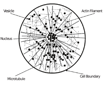
Figure 1: Two-dimensional representation of a cell with cytoskeletal structure. Adapted from [4].

Released vesicles can diffuse inside the cell, but they can also be reabsorbed by the membrane at a constant rate, later called recycling rate ([3]). Vesicles need to be transported from the cell membrane to the endosomal system located in different areas inside the cell – this transport process is called membrane trafficking (see [6]). To facilitate this process, in addition to the free diffusion, vesicles can also perform a directed motion along the cytoskeleton, which is an intracellular structure made of two different kinds of polymer filaments: actin filaments and microtubule filaments (see Figure 1). Whereas actin filaments are randomly distributed, microtubules (MT) are directed toward the microtubule organization center (MTOC), which is located close to the cell nucleus (see Figure 2). In order to perform a directed motion along actin or MT filaments, vesicles have to bind to motor proteins (kinesines, dyneins and myosins) which basically determine the type of motion. The interaction between motor proteins and their related filaments depends on several additional factors, most notably the presence of specific proteins such as Rab GTPases, scaffolding proteins and receptor proteins (see [9]). To which extent these proteins are present depends on the other hand on the genes of the cell, which have to be transcriptionally active in order to synthesize these proteins – a process called gene expression.

It is exactly this dependency, which motivates our interest in the motion of vesicles. If a given gene, for example cdk8, is transcriptionally active, it allows the synthesis of the protein CDK8, which may affect intracellular processes in various, mostly unknown ways. In this paper, we precisely ask how such a gene – through the synthesis of the specific protein – affects the motion and pattern formation of vesicles. The latter process results from the fact that vesicles can form larger ones by fusing with other vesicles. The fusion process relies on energy provided by the cell and can only take place on the MT if vesicles are close enough and below a critical size. The two simultaneous dynamic processes, namely (free or directed) motion and fusion result in a distinct spatio-temporal distribution of vesicles of different sizes - which we want to predict with our model.

The patterns produced by means of our agent-based simulation can then be compared to experiments which show such vesicle patterns depending on the transcriptional activity of specific genes (see [1]). These genes can, for example, be knocked out in RNAi or drug screens, which in turn perturb the synthesis of proteins (see [11]). Of course, such patterns can be only compared in a statistical sense, a problem discussed in the Conclusions. However, if we are able to reproduce empirical patterns with our model, we argue that the underlying dynamic processes, motion and fusion, are covered sufficiently with our modeling assumptions. This does not only hold for the assumed interaction between vesicles and MT or other vesicles, it shall also hold for particular parameter dependencies, most notably the concentration of specific proteins. Precisely, we want to end up with a testable prediction of how these concentrations affect vesicle motion and fusion, which shall be confirmed by subsequent experiments (see [1]). Some of the transition rates later used in our model specifically depend on the experimental setup, e.g. the endocytic cargo. Here we consider the case of Transferrin, an iron-binding protein contained in the vesicles to which fluorescently labelled proteins can be attached, i.e., vesicles can be made visible in the experiment. The aforementioned internalization rate and recycling rate are thus taken for Transferrin.

Eventually, we note that our modeling approach (as every modeling approach) is based on a number of simplifications: (i) we neglect the motion of vesicles along actin filaments, because it was shown [4] that such processes do not affect the pattern formation (recall that fusion only takes place on MT), (ii) we assume that the cytoskeleton is described by the spatial structure of MT only (i.e. tha actin filaments are neglected) and that MT are abundant (i.e. there are always MT to move on) and do not change in time. This allows to neglect the growth and shrinkage of MT when modeling the motion and fusion of vesicles. (iii) We neglect fission, i.e. the fragmentation of larger vesicles into vesicles of smaller sizes.

3 A Model of Brownian Agents

Brownian agents

Our modeling approach is based on the concept of Brownian agents [16] which found many interesting applications in biology [8, 7, 12, 10] but also in modeling social systems such as online communities [17]. It allows to formalize the agent dynamics using methods established in statistical physics. A Brownian agent is described by a set of state variables $u_{i}^{(k)}$, where the index $i=1,...,N$ refers to the individual agent $i$, while $k$ indicates the different variables. These could be either external variables that can be observed from the outside, or internal degrees of freedom that can only be indirectly concluded from observable actions. Noteworthy, the different (external or internal) state variables can change in the course of time, either due to influences of the environment, or due to an internal dynamics.

In the following, each agent represents an intracellular vesicle which, in accordance with the previous description, is able to change its state by spatial mobility, changes of activity, and growth processes, as formalized subsequently.

Spatial mobility

For the agent’s spatial position $r_{i}(t)$, We assume that changes in the course of time can be described by an overdamped Langevin equation of a Brownian particle moving in an effective potential [16]:

$$\frac{d\mathbf{r}_{i}}{dt}=\mathbf{v}_{i}[\theta_{i}(t)]=\frac{\alpha[\theta_{i}(t)]}{\gamma_{0}}\;\frac{\partial h^{e}(\mathbf{r},t,\theta)}{\partial\mathbf{r}}+\sqrt{2D}~{}\mathbf{\xi}_{i}(t)$$ (1)

The overdamped limit implies that the absolute value of the agent’s velocity $v_{i}$ is approximately constant, but the direction may change due to stochastic influences. Further, $\mathbf{v}_{i}$ implicitly depends on the agent’s mode of activity, $\theta_{i}(t)$.

Eqn. (1) assumes that the agent’s motion is influenced by two different forces, a deterministic one which results from the gradient of the effective potential, and a stochastic one, which is assumed to be Gaussian white noise, $\left\langle\mathbf{\xi}_{i}(t)\right\rangle=0$, $\left\langle\mathbf{\xi}_{i}(t)\mathbf{\xi}_{j}(t^{\prime})\right\rangle=\delta_{ij}\delta(t-t^{\prime})$. The strength of the stochastic force $D=k_{B}T/\gamma_{0}$ determines, in the spatial case, the diffusion coefficient, with $\gamma_{0}$ being the friction coefficient.

The deterministic part contains two important ingredients: The effective potential $h^{e}(\mathbf{r},t,\theta)$ describes the conditions inside the cell. The response function $\alpha[\theta_{i}(t)]$ depends on the internal state of the agent, $\theta_{i}(t)$ and determines what component of the effective potential actually influences the agent. Both are specified later after we made clear the notion of the internal state $\theta$.

Changes of activity

We assume that the agent’s mode of activity $\theta_{i}(t)$ can be changed, $\omega(\theta^{\prime}|\theta)$ being the transition rate from state $\theta$ into any other state $\theta^{\prime}$. In accordance with the literature [4], we distinguish five different modes of activity of a vesicle as shown in Table 1, each of which is expressed by a different value of the internal degree of freedom $\theta$.

$\theta=0$	Free diffusion in the cytosol
$\theta=1$	Kinesin-driven transport towards MT plus-ends
$\theta=2$	Dynein-driven transport towards MT minus-ends
$\theta=3$	Kinesin/Dynein-driven transport on MT with tendency to fusion with other vesicles
$\theta=4$	Bound to the cell membrane

Table 1: Different modes of activities, MT stands for microtubuli

While in principle transitions between all states could be assumed, only a subset of them is biologically relevant. Table 3 in Section 4.1 will list those together with their respective value, i.e. the expected number of transitions per time unit.

Growth and decay

We assume that fusion, i.e. the coalescence of two vesicles with sizes $s_{i}$ and $s_{j}$, can be described by a transition rate $\omega(s_{i+j}|s_{i},s_{j})$ that depends on the internal states $\theta_{j}$, $\theta_{i}$ of the agents, i.e. their ability to fuse, and their effective distance $\left|\mathbf{r}_{i}-\mathbf{r}_{j}\right|$. As described above, fusion is only possible for agents with the internal state $\theta=4$ which is expressed by the Kronecker delta, $\delta_{\theta_{i},4}$. Further, due to the volume exclusion, agents can effectively approach each other only up to a distance $d$ (which represents an average spatial extension of vesicles). The ability to fuse also depends on the vesicle size because of the energy required for this process. Because the available fusion energy is limited, it was observed experimentally that vesicles of a size larger than $s_{\mathrm{max}}$ do not fuse. This is considered in the transition rates by an additional exponential cut-off term which becomes effectively zero if one of the fusing vesicles reaches the maximum size. This leads us to the transition rate for fusion:

$$\omega(s_{i}+s_{j}|s_{i},s_{j})=\frac{\omega^{s}\delta_{\theta_{i},4}\delta_{\theta_{j},4}}{d+\left|\mathbf{r}_{i}-\mathbf{r}_{j}\right|}\cdot\frac{e^{\varepsilon(2s_{max}-s_{i}-s_{j})}}{\left[1+e^{\varepsilon(s_{max}-s_{i})}\right]\cdot\left[1+e^{\varepsilon(s_{max}-s_{j})}\right]}$$ (2)

Here $\omega^{s}$ denotes the fusion affinity which depends on the protein concentration, and $\varepsilon=0.05$ is chosen as a small number, to increase the cutoff effect.

Little is known regarding the fission process, i.e. the fragmentation of a vesicle of size $s_{l}$ into two vesicles of sizes $s_{i}$, $s_{j}$ (with $s_{l}=s_{i}+s_{j}$) . Therefore, we assume that the respective transition rate $\omega(s_{i},s_{j}|s_{i}+s_{j})$ is a constant $w$ equal for all possible fragmentation processes, which describes spontaneous fragmentation. If $w$ is small compared to other transition rates, fission can be neglected in first approximation.

We note that, because of the fusion process, the total number of vesicles, is no longer constant. While a conservation of the total mass $M$ of all vesicles can still be assumed, both the number of vesicles and their size distribution $P(N_{1},N_{2},...,N_{s}...,t)$ changes over time. Therefore, we have

$$M=\sum_{l=1}^{N}s~{}N_{s}(t)=const.~{};~{}~{}\sum_{l=1}^{N}N_{s}(t)\neq const.$$ (3)

Effective potential

After the above distinction between the different values for the internal degree of freedom $\theta$, we can now specify the effective potential which depends on these states. $h^{e}(\mathbf{r},t,\theta)$ denotes a scalar potential field that results from the influence of different field components $h_{\theta}(\mathbf{r},t)$. Each of these components refers to specific conditions inside the cell. Compared to the time scale involved in the motion of the vesicles, some of these conditions can be assumed as constant in time, but varying across space.

With reference to Table 1, $h_{4}(\mathbf{r})$ describes the influence of the cell membrane on the motion of agents in state $\theta=4$ as they can bind to the membrane. $h_{{}^{1}}(\mathbf{r})$ and $h_{2}(\mathbf{r})$ determine the agent’s motion along the microtubule filaments. $h_{0}(\mathbf{r})$ on the other hand represents the cell topology, i.e. it generates a repelling force close to the cell membrane and to the nucleus, but is is simply a constant inside the cell, because free diffusion inside the cell should not be affected.

The only time-dependent component of the effective field is $h_{3}(\Delta\mathbf{r},t)$, which affects the fusion processes between vesicles (fission neglected). In fact, this is a short range attraction potential which increases with decreasing distance $\Delta\mathbf{r}=\left|\mathbf{r}_{i}-\mathbf{r}_{j}\right|$. Since agents move, $h_{3}$ changes in time depending on their actual positions $\mathbf{r}_{i}(t)$ and internal states $\theta_{i}(t)$.

In order to describe how the effective potential results from the different field components, we have to consider the response function $\alpha[\theta_{i}(t)]$ that determines which of the field components are actually “seen” by the agents conditional on their internal states. In accordance with the above distinction, we specify:

$$\alpha[\theta_{i}(t)]~{}h^{e}(\mathbf{r},\theta,t)=\alpha_{0}h_{0}(\mathbf{r}) +\delta_{\theta_{i},1}~{}\alpha_{1}h_{1}(\mathbf{r})+\delta_{\theta_{i},2}~{}\alpha_{2}h_{2}(\mathbf{r})$$

$$+\delta_{\theta_{i},4}~{}\alpha_{4}h_{4}(\mathbf{r})+\delta_{\theta_{i},3}~{}\alpha_{3}h_{3}(\Delta\mathbf{r},t)$$ (4)

The different $\alpha_{k}$ are dimensional constants. With eqn. (3) the motion of every agent is specified according to eqn. (1). We point out that agents with $\theta_{i}=0$ behave like simple Brownian particles which are not affected by any conditions inside the cell, except for the boundary conditions.

Master equation

The state of each individual agent is now described by a triple of three different state variables $\{r_{i}(t),\theta_{i}(t),s_{i}(t)\}$ that can change in time according to the processes specified above. The multi-agent system is thus described by the grand-canonical $N$-particle distribution function

$$P_{N}=P_{N}(\underline{\mathbf{r}},\underline{\theta},\underline{s},t)=P_{N}(\mathbf{r}_{1},\theta_{1},s_{1},...,\mathbf{r}_{N},\theta_{N},s_{N},t),$$ (5)

which describes the probability density of finding $N$ Brownian agents with the distribution of internal parameters $\underline{\theta}$, positions $\underline{r}$ and sizes $\underline{s}$ at time $t$. Note that $N$ is not constant but can change over time due to fusion (and fission) events.

The complete dynamics for the ensemble of agents can be formulated in terms of a multivariate master equation:

$$\frac{\partial}{\partial t}P_{N}(\underline{\mathbf{r}},\underline{\theta},\underline{s},t)= -\sum_{i=1}^{N}\left\{\mathbf{\nabla}_{i}\left[\frac{\alpha[\theta_{i}(t)]}{\gamma_{0}}~{}\mathbf{\nabla}_{i}h^{e}(\mathbf{r},t,\theta)P_{N}(\underline{\mathbf{r}},\underline{\theta},\underline{s},t)\right]-D\mathbf{\Delta}_{i}P_{N}(\underline{\mathbf{r}},\underline{\theta},\underline{s},t)\right\}$$ (6a)

$$+\sum^{N}_{i=1}\sum_{\theta_{i}^{\prime}\neq\theta_{i}}\left[\omega(\theta_{i}|\theta_{i}^{\prime})~{}P_{N}(\underline{\mathbf{r}},\theta_{i}^{\prime},\underline{\theta}^{*},\underline{s},t)-\omega(\theta_{i}^{\prime}|\theta_{i})P_{N}(\underline{\mathbf{r}},\underline{\theta},\underline{s},t)\right]$$ (6b)

$$+\sum^{N}_{i=1}\sum_{i<j}\left[\omega(s_{i}+s_{j}|s_{i},s_{j})P_{N+1}(\underline{\mathbf{r}}^{*},\theta_{i}=3,\theta_{j}=3,\underline{\theta}^{*},\underline{s}^{*},t)\right.$$

$$\left.-\omega(s_{i},s_{j}|s_{i}+s_{j})P_{N}(\underline{\mathbf{r}},\theta_{i}=3,\theta_{j}=3,\underline{\theta},\underline{s},t)\right]$$ (6c)

The first part of the multivariate master eqn., (6a), describes changes of the probability distribution due to movements of agents either by diffusion or following some gradients of the effective field. The second part, (6b), considers all possible changes of the distribution of internal states, $\underline{\theta}$, where $\underline{\theta}^{*}$ denotes “neighboring” states that differ from $\underline{\theta}$ only by the element explicitly given. The third part, (6c), eventually describes the fusion process by any two agents. This leads to a “gain” if the total number of vesicles is decreased by $N+1\to N$ and distribution changes result in $\underline{r}^{*}\to\underline{r}$, $\underline{s}^{*}\to\underline{s}$, or to a “loss” for any other process with $N\to N-1$.

The multivariate master equation has the advantage of considering all possible processes on the agent level in a stochastic framework. After completely specifying the transition rates involved, we are able to solve this equation by means of stochastic computer simulations (see Section 4.4).

We note that from eqn. (6), one can in principle derive a macroscopic density equation by introducing the agent density of the grand-canonical ensemble:

$$n(\mathbf{r},t)=\sum_{N=1}^{\infty}N\int dr_{1}...dr_{N-1}P_{N}(r_{1},...,r_{N-1},r,t)$$ (7)

The resulting equation would have the known structure of a reaction-diffusion equation for $n(\mathbf{r},t)$. While this may be the “classical” way of investigation, we point out that for the agent-based approach proposed here the stochastic framework is the more appropriate one because it refers to the individual processes on the agent level. We emphasize that the agent-based approach is better suited for computer simulations of spatiotemporal patterns because it provides a stable and fast numerical algorithm. This becomes especially important in the case of large density gradients, which may considerably decrease the time step allowed to integrate the related dynamics.

4 Setup for stochastic simulations

4.1 Velocities and transition rates

According to the distinction between the activity modes given in Table 1, the movement of the agents can be of two types: free motion by diffusion processes, described by the diffusion coefficient $D$, and bound motion along the microtubuli. Both types are described by eqn. (1). In order to calculate the different $\mathbf{v}_{i}(\theta)$, we would need to specify explicitly the related components of the effective potential, $h_{\theta}(\mathbf{r},t)$ that result in the directed motion along the microtubuli. To simplify the procedure and match it with experimental findings, we may instead consider the value of $v_{i}(\theta)$ as given by experiments. Then, the role of the field component is reduced to simply keep the agents on the microtubuli as long as they are in the respective internal states $\theta$. I.e. both $\nabla_{i}h_{1}(\mathbf{r})$ and $\nabla_{i}h_{2}(\mathbf{r})$ just determine the direction of motion along the microtubulus to which agent $i$ is attached, whereas $h_{0}(\mathbf{r})$ specifies the boundary condition given by the location of the cell nucleus and the cell membrane (see also Figure 2). Table 2 provides the values for the velocities which are assumed to be constant and the same for all agents in the respective internal state.

State	Parameter value	Description
$\theta=0$	$D=10^{-15}~{}\rm m^{2}/s$	Diffusion coefficient in cytoplasma
$\theta=1$	$v_{1}=0.33~{}\rm\mu m/s$	Velocity of vesicle on MT towards plus-ends
$\theta=2$	$v_{2}=0.33~{}\rm\mu m/s$	Velocity of vesicle on MT towards minus-ends

Table 2: Parameters describing the free ($\theta=0$) or bound ($\theta=1,2$) motion of agents. MT means ‘microtubulus’. Note that the diffusion coefficient is related to the friction coefficient via $\gamma_{0}=k_{B}T/{D}$, which results in $\gamma_{0}=4\cdot 10^{-6}\rm kg/s$. Values according to [5].

As a next step, we need to specify the transition rates $\omega(\theta^{\prime}|\theta)$ between different modes of activity. Again, instead of providing explicit expressions, we may simply take values obtained from experiments. These values are available to us only for the unperturbed state of the cell, i.e. for a baseline or reference case in which conditions inside the cell are not changed on purpose. In the following, baseline values are indicated by the superscript $b$. Table 3 lists all biologically relevant transition rates for the unperturbed scenario, as obtained either from the literature or from own experiments.

Parameter Value	Description
$\omega^{b}(1|0)$=0.05 $\rm s^{-1}$	Transition from diffusive to MT (plus-end) bound state
$\omega^{b}(0|1)$=0.33 $\rm s^{-1}$	Transition from MT-bound (plus-end) to diffusive state
$\omega^{b}(2|0)$=0.05 $\rm s^{-1}$	Transition from diffusive to MT (minus-end) bound state
$\omega^{b}(0|2)$=0.33 $\rm s^{-1}$	Transition from MT (minus-end) bound to diffusive state
$\omega^{b}(3|1)$=0.01 $\rm s^{-1}$ ⋆	Transition from MT-bound to MT-bound state with fusion
$\omega^{b}(1|3)$=0.02 $\rm s^{-1}$ ⋆	Transition from MT-bound state with fusion to MT-binding
$\omega^{b}(3|2)$=0.01 $\rm s^{-1}$ ⋆	Transition from MT-bound to MT-bound state with fusion
$\omega^{b}(2|3)$=0.02 $\rm s^{-1}$ ⋆	Transition from MT-bound state with fusion to MT-binding
$\omega^{b}(0|4)$=0.0025-0.0033 s-1	Internalization rate of vesicles
$\omega^{b}(4|0)$=0.00083-0.0012 s-1	Recycling rate of vesicles

Table 3: Biologically relevant transition rates $\omega^{b}(\theta^{\prime}|\theta)$ for the baseline case (unperturbed concentrations of proteins). Values according to [5], values with ^⋆ are from own experiments, see [1].

4.2 Reduced transition rates

The given set of transition rates leaves us with a large degree of freedom which however turns out to be a pitfall: if we wanted to compare the simulations with patterns observed in the experiment, we would need to raster the full parameter space to find appropriate combinations of transition rates which lead to a realistic outcome. There are basically two ways to reduce this parameter space: (i) we use known values of the transition rates as e.g. reported in the literature, (ii) we introduce reduced transition rates, assuming that not all processes are really independent. We follow a combination of the two, defining the reduced transition rates as given in Table 4

$\Omega_{1}=\frac{\displaystyle\omega(1|0)}{\displaystyle\omega(0|1)}$	Affinity for microbule plus-ends
$\Omega_{2}=\frac{\displaystyle\omega(2|0)}{\displaystyle\omega(0|2)}$	Affinity for microbule minus-ends
$\Omega_{3}=\frac{\displaystyle\omega(3|1)}{\displaystyle\omega(1|3)}$	Fusion tendency on microbule plus-ends
$\Omega_{4}=\frac{\displaystyle\omega(3|2)}{\displaystyle\omega(2|3)}$	Fusion tendency on microbule minus-ends
$\Omega_{5}=\frac{\displaystyle\omega(0|4)}{\displaystyle\omega(4|0)}$	Internalization versus recycling rate

Table 4: Reduced transition rates $\Omega_{i}$, to combine two transition rates $\omega$ which refer to the same intracellular (transport) mechanism but describe inverse processes.

In the following we assume that $\Omega_{3}=\Omega_{4}\equiv\Omega_{F}$ which denotes the fusion tendency that is supposed to be independent of the kind of motor protein involved (this was kinesin for $\Omega_{3}$ and dynein for $\Omega_{4}$). With this, we finally have reduced the transition rates to 4 parameters given by $\Omega_{1},\Omega_{2},\Omega_{F}$ and $\Omega_{5}$.

These reduced parameters of course do not fully determine the individual transition rates which are needed to recover the correct dynamics. Therefore, for one of the transition rates we use the baseline value from the literature, as given by Table 3. So, we define e.g. $\Omega_{1}=\omega(1|0)/\omega^{b}(0|1)$ or $\Omega_{1}=\omega^{b}(1|0)/\omega(0|1)$.

Eventually, we want to emphasize the distinction between the reduced transtion rates $\Omega_{i}^{u}$ for the unperturbed case (control cell) and $\Omega^{k}_{i}$ for the perturbed case, where the protein $k$ was manipulated. Similar to the discussion in Section 4.1, they refer to the same transition rates $\omega$, but with different concentrations $c_{k}$.

4.3 Boundary and initial conditions

In order to complete the setup for the stochastic computer simulations, we still need to specify the boundary conditions which refer to the cell geometry. Figure 2 (a,b) shows the two different cell geometries chosen, a rather circular cell and an elongated one. The outer boundary of the cell membrane and the inner boundary of the nucleus are both assumed to be impermeable walls, described by a hard sphere potential $h_{0}(\mathbf{r})$.

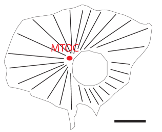
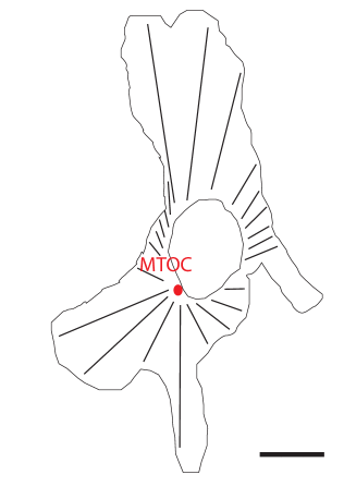
Figure 2: (left) (a) Circular geometry of a non-treated (control) cell; (right) (b) Elongated geometry of a perturbed cell (treated with siRNA, which leads to the depletion of CDK8). The scale bar corresponds to 5$\mu m$. The microtubule filaments are schematically sketched, pointing toward the MTOC (microtubule organization center). Vesicle in an internal state $\theta\in\{1,2,3\}$ move along microtubules in both directions.

The interior of the cell contains the cytoskeleton, i.e. both actin filaments and microtubuli (MT) which provide boundary conditions for the motion of vesicles (see also Figure 1). As already discussed, we do not consider motion along actin filaments because the related processes do not contribute to vesicle pattern formation. MT, on the other hand, are abundant and always point to the microtubule organization center (MTOC) which is assumed to be in the perinuclear area on the side with the largest part of the cytosol (see Figure 2 a,b).

Regarding the initial conditions, we need to specify the number, the position, the internal state and the size of the agents at $t=0$. For our model, we assume that initially all vesicles are bound to the cell membrane, i.e. at $t=0$ agents start with $\theta_{i}(0)=4$ at a position $\mathbf{r}_{i}(0)$ randomly chosen from the cell boundary. In order to determine the initial number of agents, we start from the experimental observation that an average cell (of the type considered) contains about 200 internalized vesicles at steady state. This number excludes vesicles still bound to the cell membrane. We further know from experiments that internalization rates, i.e., transition rates from the initial bound into the free moving state (and vice versa), i.e. $\omega(0|4)=3.3\cdot 10^{-3}\rm s^{-1}$ and $\omega(4|0)=8.3\cdot 10^{-4}\rm s^{-1}$ (see Table 3). If $N(0)=N_{4}(0)$ denotes the (unknown) number of agents at $t=0$ (all assumed to be in the bound state) and $N(0)-N_{4}^{st}=200$ the (known) number of agents no longer in the bound state at steady state ($st$ : steady state), then we can postulate for the dynamics for $N_{4}(t)$ the following rate equation:

$$\frac{dN_{4}(t)}{dt}=-\omega(0|4)~{}N_{4}(t)+\omega(4|0)~{}\left[N_{4}(0)-N_{4}(t)\right]$$ (8)

After a time $t\sim 1/[\omega(0|4)+\omega(4|0)]$, this dynamics reaches a steady-state solution

$$N_{4}^{st}=\frac{\omega(4|0)}{\omega(0|4)+\omega(4|0)}N_{4}(0)$$ (9)

from which we can calculate $N_{4}(0)$ assuming that $N(0)-N_{4}^{st}=200$. This approximation neglects the fact that the total number of vesicles have decreased at time $t$ because of the fusion between vesicles. Thus, we may slightly increase the initial number of agents and have eventually chosen $N_{4}(0)=350$.

It remains to determine the initial distribution of vesicle sizes. We want to start from a most realistic one because (a) later we want to compare the time scale of structure formation with the experimental observation, and (b) because our modeling setup has neglected the fragmentation rate of vesicles (which would be needed if an arbitrary initial distribution needs to relax into a realistic one). Again, we rely on experimental observations [1] that have found a log-normal distribution of vesicle sizes:

$$P(s;\mu,\sigma)=\frac{1}{s\sigma\sqrt{2\pi}}\exp{\left\{-\frac{(\ln s-\mu)^{2}}{2\sigma^{2}}\right\}},$$ (10)

where $\mu$ and $\sigma$ are the mean and standard deviation of the variable’s natural logarithm.

4.4 Stochastic Simulation Technique

We now have determined all ingredients for stochastic computer simulations which include the following dynamic processes (specified on the agent level):

Initialization

At $t=t_{0}$, 350 agents with $\theta_{i}(0)=4$ are randomly placed at the cell boundary. Their initial size $s_{i}(0)$ is drawn from the log-normal distribution, (10).

Movement

Agents can change from the bound state into the free moving state at a rate $\omega(0|4)$ and from the free moving state into directed motion at rates $\omega(1|0)$, $\omega(2|0)$. They all move according to the equation of motion, (1).

In our modeling approach, only agents with the internal states $\theta\in\{1,2,3\}$ move along the MT. We assume that, whenever an agent switches from $\theta=0$ into either $\theta=1$ or $\theta=2$, i.e. from a free motion into a bound motion, a MT is “always at hand”. If the agent switches from $\theta\in\{1,2\}$ into $\theta=3$ where it is ready to fuse, it continues to move into the same direction as before, until it collides with another agent.

Fusion

Precisely, fusion occurs only on MT. Agents need to be in state $\theta=3$ and in a sufficiently close distance. After fusion, the smaller agent “disappears”, whereas the larger one has increased its size, but keeps the internal state $\theta=3$ until one of the transitions $\omega(2|3)$ or $\omega(1|3)$ happen.

Inversion

Agents bound to the MT can become freely moving at the rates $\omega(0|2)$, $\omega(0|1)$, whereas free moving agents can be bound again to the cell membrane at the rate $\omega(4|0)$.

Concurrency

We assume that agents can move and transit into different internal states at the same time. This allows us to decouple the motion of agents from the various reactions (change of internal states and fusion).

The state of the multi-agent system is at any time completely described by the $N$-particle distribution function $P_{N}(\underline{\mathbf{r}},\underline{\theta},\underline{s},t)$. However, because of the dynamical processes, the system state always changes and its average “life time” $\mathcal{T}_{m}$ is just the inverse of the sum over all possible transition rates that can change the given state (including changes of position, internal states, and sizes).

Because we have to deal with movement and reactions at the same time, we have chosen a sufficiently small fixed time interval $\Delta t=0.02s$ to solve the equations of motion of each individual agent. To answer the question if in the respective time interval also a change of the internal states or a fusion process occurs, we proceed as follows:

Each of the possible reactions has a different probability to occur, which is determined by the respective transition rate and the available time, $\Delta t$. In order to pick one of the possible reactions, we draw a uniformly distributed random number $U\in\textrm{RND}[0,1]$ and choose the process $z$ that satisfies the condition

$$\sum_{j=0}^{z}\omega_{z}(\cdot)\Delta t<U<\sum_{j=0}^{z+1}\omega_{z}(\cdot)\Delta t$$ (11)

Because $\Delta t$ was chosen such that $\sum_{n=1}^{N}\omega_{n}(\cdot)\Delta t\leq 1$, none of the possible processes is excluded from being picked. On the other hand, it may occur that none of the processes is being chosen if the sum is much smaller than 1 and $U$ close to 1. Then no reaction occurs during the respective time interval, but movements take place.

5 Results

5.1 Spatio-temporal vesicle patterns

Figure 3 presents computer simulations of the vesicle patters for both the unperturbed (control) cell and the perturbed cell (cf also Figure 2). We emphasise that these simulations refer to real spatial and time scales, so they should be comparable, at least in a statistical sense, to patterns observed from experiments. These experiments are reported in [1] and have motivated the choice of the reduced transition rates, $\Omega_{i}$, which are treated in this paper as free parameters.

Comparing the pattern formation in the perturbed cell with the one in the control cell, we note a number of differences: we observe a localization of large vesicles on the one hand at the tips of the elongated branched-out perturbed cell, on the other hand large vesicles are as well localized in the perinuclear area of this cell. In the unperturbed cell, the majority of large vesicles are located around the nucleus and vesicles are spread over the entire cell surface getting more sparse towards the cell periphery.

Comparing the vesicle size distribution of both the perturbed and the unperturbed cell, we find that they preserve the form of the log-normal distribution, but the mean value $\mu$, in the course of time, shifts to significant larger values in the perturbed cell (see also Table 5). The perturbed cell displays a geometry that may have facilitated fusion of vesicles in its branches within which they accumulate. The transport of vesicles from these branches to the nucleus of the perturbed cell seems to be suppressed.

$t$	1 min	5 min	10 min	15 min
$\mu^{u}$	2.69	2.82	2.94	2.96
$\sigma^{u}$	0.89	0.94	0.94	0.96
$\mu$	2.87	2.99	3.00	3.04
$\sigma$	0.90	0.90	0.94	0.86

Table 5: Mean $\mu(t)$ and standard deviation $\sigma(t)$ of the log-normal distribution at different times $t$ (min) for the unperturbed (superscript $u$) and the perturbed cell.

        1 min 5 min 10 min 15 min       

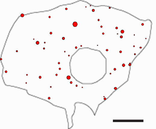
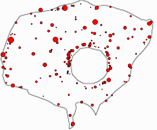
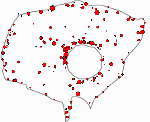
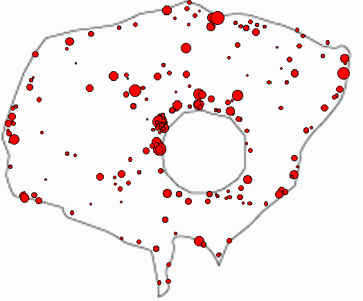
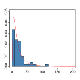
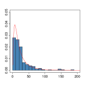
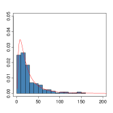
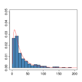
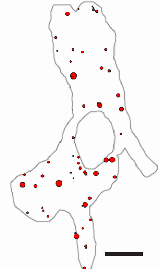
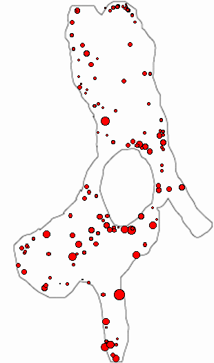
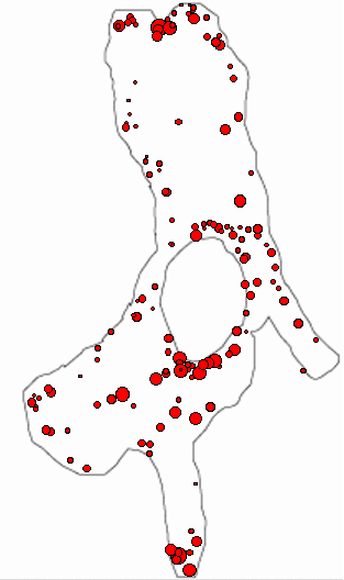
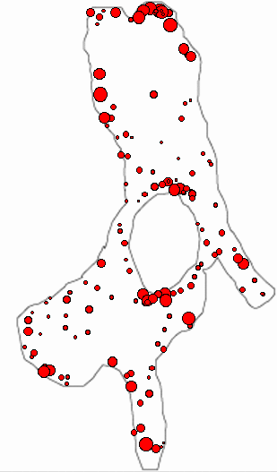
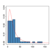
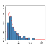
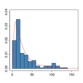
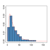
Figure 3: Computer simulations of vesicle patterns on real time scale (in min) and spatial scale (scale bar: 5$\mu$m ). (top) unperturbed cell: $\{\Omega_{1},\Omega_{2},\Omega_{F},\Omega_{5}\}$=$\{0.925,1.1,1.0,0.85\}$, (bottom) perturbed cell: $\{\Omega_{1},\Omega_{2},\Omega_{F},\Omega_{5}\}$=$\{1.3,1.2,1.2,0.55\}$. The histograms show the evolution of the vesicle size distribution together with the fitted log-normal distribution (red line). Values for $\mu$ and $\sigma$ are given in Table 5.

5.2 Estimating concentration dependence

As pointed out above, we found very realistic vesicle patterns both for the perturbed and the control cell for the given set of reduced transition rates $\Omega_{i}$ (see Figure 3). These transition rates are treated as free parameters in our model – but provided they are correct (which can only be confirmed by comparing the patterns with experiments, statistically) they allow an indirect estimation of the concentration dependence of the transition rates $\omega(\theta^{\prime}|\theta)$.

As already stated, the transition rates are given to us only for the unperturbed state of the cell. Table 3 presents the values for the baseline case. One should note, however, that the baseline value not necessarily describes the experimental situation because it was obtained under conditions which are hardly reproducible completely. If we for example change the concentration $c_{k}$ of some protein ${k}$ inside the cell which is involved in processes of fusion or directed motion, this will certainly change the value of the respective transition rates, i.e. $\omega=\omega(c_{k},c_{l},...)$. Hence, it is not only sufficient to know the values of the baseline case, we should also know how these values of the transition rates change with the concentrations $c_{k}$. If we denote the transition rates in the unperturbed case by $\omega^{u}$ (omitting the $\theta$ dependence at the moment) and the respective protein concentrations by $c^{u}$ we may assume in first-order approximation the following expansion:

$$\omega(c_{k},c_{l\neq k}=c^{u}_{l\neq k})=\omega^{u}(c_{k}^{u},c^{u}_{l\neq k})+\left.\frac{\partial\omega}{\partial c_{k}}\right|_{c_{k}^{u}}(c_{k}-c_{k}^{u}).$$ (12)

To further specify the functional dependency $\omega(c_{k})$ we make the following ansatz:

$$\omega(c_{k},c_{l\neq k}=c^{u}_{l\neq k})=\omega^{u}\cdot\exp\left(\kappa_{k}\frac{c_{k}-c_{k}^{u}}{c_{k}^{u}}\right).$$ (13)

which satisfies $\omega(c_{k},c_{l\neq k}=c^{u}_{l\neq k})=\omega^{u}$ for $c_{k}=c_{k}^{u}$. The important parameter $\kappa_{k}$ denotes the impact that a change of concentration $c_{k}$ has on the respective transition rate, i.e. it is a measure of sensitivity toward that particular protein. Of course, $\kappa_{k}=\kappa_{k}(\theta^{\prime}|\theta)$ in full notation, i.e. the value does not only change across proteins, but the impact also changes for different transitions. Putting eqs. (12), (13) together, we arrive at:

$$\Delta\omega_{k}=\omega(c_{k},c_{l\neq k}=c^{u}_{l\neq k})-\omega^{u}=\omega^{u}\frac{\kappa_{k}}{c_{k}^{u}}(c_{k}-c_{k}^{u})$$ (14)

In many experimental cases, as e.g. in RNAi screens, the perturbation of a protein concentration leads to $c_{k}\to 0$, i.e. we are interested in the dynamics in the absence of a given protein. With this assumption we finally have:

$$\Delta\omega_{k}(\theta|\theta^{\prime})=-\kappa_{k}(\theta|\theta^{\prime})~{}\omega^{u}(\theta|\theta^{\prime}).$$ (15)

This allows us to relate two different dynamical scenarios and their respective outcome in terms of the vesicle patterns: (i) the unperturbed scenario with experimentally known concentrations and known transition rates, and (ii) the perturbed scenario, where different proteins may be absent.

As an example, let us investigate how changes in the concentration $c_{k}$ of the protein $k=\mathrm{CDK8}$ affect the transition rates $\omega_{\mathrm{CDK8}}(1|0)$ and $\omega_{\mathrm{CDK8}}(0|1)$. Given the parameters in Figure 3, the reduced transition rates return $\Omega_{1}^{\mathrm{CDK8}}-\Omega_{1}^{u}=0.375$, where $\Omega_{i}^{\mathrm{CDK8}}$ refers to the case where the protein concentration $c_{k}=c_{\mathrm{CDK8}}=0$, whereas $\Omega_{i}^{u}$ refer to the unperturbed case. Dividing eqn. (15) by $\omega^{b}(0|1)$, we find

$$\Delta\Omega_{1}^{\mathrm{CDK8}}=\Omega_{1}^{\mathrm{CDK8}}-\Omega_{1}^{u}=0.375 =-\frac{\omega^{u}(1|0)}{\omega^{b}(0|1)}\cdot\kappa_{\mathrm{CDK8}}(1|0)$$

$$=-\Omega_{1}^{u}\cdot\kappa_{\mathrm{CDK8}}(1|0),$$ (16)

from where it follows that $\kappa_{\mathrm{CDK8}}(1|0)\approx-0.41$, which describes the sensitivity toward changes in the concentration of CDK8.

Knowing the difference $\Delta\Omega_{1}^{\mathrm{CDK8}}$, the transition rates $\omega_{k}$ are not fully determined because of $\Omega_{1}^{u}=\omega^{u}(1|0)/\omega^{b}(0|1)$, $\Omega_{1}^{\mathrm{CDK8}}=\omega_{\mathrm{CDK8}}(1|0)/\omega^{b}(0|1)$. Hence, we can now discuss two different cases which refer to two hypotheses about the transport of vesicles towards microtubule minus-ends.

The first hypothesis of our model states that the transition rate $\omega_{\mathrm{CDK8}}(1|0)$ in cells that are silenced for CDK8 reads:

$$\omega_{\mathrm{CDK8}}(1|0)=\omega^{u}(1|0)\cdot\exp\bigg{(}-0.41\cdot\frac{c_{\mathrm{CDK8}}-c_{\mathrm{CDK8}}^{u}}{c_{\mathrm{CDK8}}^{u}}\bigg{)}.$$ (17)

Assuming $c_{\mathrm{CDK8}}\approx 0$, it follows, that $\omega_{\mathrm{CDK8}}(1|0)$ is increased by a factor of approximately 1.5 with respect to $\omega^{u}(1|0)$. This means that silencing the protein CDK8 increases the transition of vesicles freely diffusing in the cytosol to vesicles being transported towards the MT-plusends. We thus hypothesize that CDK8 is either directly or indirectly involved in the docking of vesicles on microtubule filaments via kinesins.

On the other hand, $\kappa_{\mathrm{CDK8}}(0|1)$ can be obtained by the following relation:

$$\Omega_{1}^{CDK8}-\Omega_{1}^{u}=0.375 =\frac{\omega^{b}(1|0)}{\omega^{CDK8}(0|1)}\cdot\kappa_{\mathrm{CDK8}}(0|1)$$

$$=\Omega_{1}^{CDK8}\cdot\kappa_{\mathrm{CDK8}}(0|1),$$ (18)

from where it follows that $\kappa_{\mathrm{CDK8}}(0|1)\approx 0.29$. The second hypothesis of our model states that the transition rate $\omega_{\mathrm{CDK8}}(0|1)$ in cells that are silenced for CDK8 reads:

$$\omega_{\mathrm{CDK8}}(0|1)=\omega^{u}(0|1)\cdot\exp\bigg{(}0.29\cdot\frac{c_{\mathrm{CDK8}}-c_{\mathrm{CDK8}}^{u}}{c_{\mathrm{CDK8}}^{u}}\bigg{)}.$$ (19)

Setting $c_{\mathrm{CDK8}}\approx 0$, we find that $\omega_{\mathrm{CDK8}}(0|1)$ is decreased by a factor of approximately 0.75 with respect to $\omega^{u}(0|1)$. This means that silencing the protein CDK8 leads to a decrease in transition of vesicles transported towards the MT-plusends to vesicles freely diffusing vesicles. We thus hypothesize that CDK8 may as well be involved in the undocking of vesicles bound to MT filaments via kinesins.

In a similar manner, we could estimate the concentration dependence of other transition rates, using the scaled transition rates $(\Omega^{CDK8}_{2},\Omega^{CDK8}_{F},\Omega^{CDK8}_{5})$ and $(\Omega^{u}_{2},\Omega^{u}_{F},\Omega^{u}_{5})$. This enables us to further develop a number of hypotheses regarding the effect of silencing the protein CDK8 on the intracellular transport.

6 Discussion

6.1 Motivation of the model

Genomic and pharmaceutical research nowadays heavily relies on systematic screens in which the perturbation or silencing of specific proteins affects the abundance of vesicle patterns observed in a population of cells. The study of vesicle pattern formation thus is important to improve our understanding of the function of genes. To learn how vesicle patterns are formed, we have set up an agent-based model of intracellular transport inside a single cell. Agents represent vesicles which move either by diffusion in the cytosol or are transported along the cytoskeletal filaments through molecular motors. Vesicles further interact with other vesicles by fusion or fission, or they interact with the cytoskeletal filaments, the cell membrane and the nucleus. This interaction is controlled and regulated by specific proteins which are synthesised inside the cell by transcriptionally active genes. The activity of these genes thus represents the control parameters of our system.

Treating vesicles as Brownian agents with an internal degree of freedom allows to formally derive a model that captures all relevant processes in the formation of vesicle patterns. Five different values of the internal degree of freedom define the vesicle’s different modes of activity. Transitions between these modes occur as stochastic events related to the binding of proteins to the vesicle’s coat, or to signalling events. Proteins involved in those processes can control the vesicle’s activity which in turn determines the process of pattern formation. We therefore assume that the transition rates between different value of the internal degree of freedom depend on the concentration of a cell’s proteins. To determine the precise transition rates as functions of protein concentrations would require the full knowledge about the regulatory structure of gene networks. We simplified this situation by assuming that the transition rates can be decomposed into a product of the unperturbed transition rates and an exponential function depending on the concentration of single proteins. We further simplified our model by assuming that the cell membrane, the cytoskeletal filaments and the nucleus are static and that the diffusion coefficient and velocities along cytoskeletal filaments are constant parameters of the model. In contrast, the transition rates represent the free parameters of our model and have been varied. We have reduced the number of 10 original transition rates to 4 scaled transition rates. This introduced an ambiguity in the interpretation of the simulation results with respect to the original transition rates. We could cope with this situation by deriving two complementary hypothesis about the influence of the proteins involved, which could be tested experimentally.

6.2 Possible comparison with experiments

In order to relate our computer simulations to reality, experimental data are needed to calibrate the simulations. Whenever available, baseline values for the transition rates obtained from experiments have been included. This allowed us to generate patterns on real time and spatial scales. From every simulated pattern, four features can be obtained: size, relative distance to nucleus, number of vesicles within a fixed radius around each vesicle and number of vesicles per cell area. To measure the dissimilarity between the simulated pattern and the experimentally observed one, it is useful to compute the symmetrized Kullback-Leibler divergence of the two corresponding vesicle feature distributions [1], to find out for which parameters the simulated pattern provides a minimum divergence to the experimentally observed vesicle patterns. An interpretation of these findings in comparison with hypotheses generated from the computer simulations allows to draw conclusions about the underlying processes, in particular about the role of the genes involved.

A comparison of simulated and experimentally measured vesicle patterns also involves a dimensional problem: our simulations are performed in 2d, whereas experimental patterns result from vesicle motion in 3d. In principle, this would require to correct for the distances as consequence of the projection from 3d to 2d. Since mammalian cells are relatively flat with the exception of the nucleus area, we have omitted this correction. But we considered the fact that vesicles could pass below/above each other by not assuming mutual exclusion in our 2d simulations.

6.3 Future directions

We emphasize again that our computer simulations lead to testable hypotheses about the influence of specific genes, such as CDK8, on the formation of vesicle patterns. One future application of our model of intracellular transport concerns the silencing of multiple genes. Let us denote with $i$ and $l$ two genes which are silenced, then according to ansatz in eqn. (13) we find for the transition rates

$$\omega_{i;l}(\theta_{j}^{\prime}|\theta_{j})=\omega(\theta_{j}^{\prime}|\theta_{j})\cdot\exp\bigg{(}\kappa_{i}(\theta_{j}^{\prime}|\theta_{j})\frac{c_{i}-c_{i}^{u}}{c_{i}^{u}}+\kappa_{l}(\theta_{j}^{\prime}|\theta_{j})\frac{c_{l}-c_{l}^{u}}{c_{l}^{u}}\bigg{)}.$$ (20)

Once we have determined $\kappa_{i}(\theta_{j}^{\prime}|\theta_{j})$ and $\kappa_{l}(\theta_{j}^{\prime}|\theta_{j})$ from single gene silencing experiments and their related simulations of our model of intracellular transport, we can predict the resulting pattern and dynamics of the combined silencing of these two genes. However, (eq. 20) is only valid, if genes $i$ and $l$ are not in the same (regulatory) pathway. Such a prediction represents an in-silico experiment and can be tested experimentally.

Acknowledgment

M.B. could benefit from numerous stimulating discussions with Lucas Pelkmans.

References

- Birbaumer [2010] Birbaumer, M. (2010). Statistical analysis and modeling of endocytic vesicle pattern formation. Ph.D. thesis, ETH Zurich, Disseration Nr. 19322.
- Conner and Schmid [2003] Conner, S.; Schmid, S. (2003). Regulated portals of entry into the cell. Nature 422(5875), 37–47.
- Dautry-Varsat [1986] Dautry-Varsat, A. (1986). Receptor-mediated endocytosis: the intracellular journey of transferrin and its receptor. Biochimie 68, 375–81.
- Dinh et al. [2006] Dinh, A.-T.; Pangarkar, C.; Theofanous, T.; Mitragotri, S. (2006). Theory of Spatial Patterns of Intracellular Organelles. Biophysical Journal 90(10), L67–L69.
- Dinh et al. [2007] Dinh, A.-T.; Pangarkar, C.; Theofanous, T.; Mitragotri, S. (2007). Understanding Intracellular Transport Processes Pertinent to Synthetic Gene Delivery via Stochastic Simulations and Sensitivity Analyses. Biophysical Journal 92(3), 831–846.
- Doherty and McMahon [2009] Doherty, G.; McMahon, H. (2009). Mechanisms of Endocytosis. Annual Review of Biochemistry 78, 857–902.
- Ebeling and Schweitzer [2003] Ebeling, W.; Schweitzer, F. (2003). Self-Organisation, Active Brownian Dynamics, and Biological Applications. Nova Acta Leopoldina NF 88(332), 169–188.
- Ebeling et al. [1999] Ebeling, W.; Schweitzer, F.; Tilch, B. (1999). Active Brownian particles with energy depots modeling animal mobility. Biosystems 49(1), 17 – 29.
- Fiore and Camilli [2001] Fiore, P. D.; Camilli, P. D. (2001). Endocytosis and Signaling: An Inseparable Partnership. Cell 106(1), 1 – 4.
- Garcia et al. [2011] Garcia, V.; Birbaumer, M.; Schweitzer, F. (2011). Testing an agent-based model of bacterial cell motility: How nutrient concentration affects speed distribution. European Physical Journal B 82(3-4), 235–244.
- Hannon [2002] Hannon, G. (2002). RNA interference. Nature 418(6894), 244–251.
- Mach and Schweitzer [2007] Mach, R.; Schweitzer, F. (2007). Modeling Vortex Swarming In Daphnia. Bulletin of Mathematical Biology 69, 539–562.
- Marsh and Helenius [2006] Marsh, M.; Helenius, A. (2006). Virus entry: open sesame. Cell 124(4), 729–740.
- Mercer and Helenius [2008] Mercer, J.; Helenius, A. (2008). Vaccinia Virus Uses Macropinocytosis and Apoptotic Mimicry to Enter Host Cells. Science 320(5875), 531–535.
- Roth [2006] Roth, M. (2006). Clathrin-mediated endocytosis before fluorescent proteins. Nat Rev Mol Cell Biol 7, 63–68.
- Schweitzer [2003] Schweitzer, F. (2003). Brownian Agents and Active Particles: Collective Dynamics in the Natural and Social Sciences. Springer, Berlin.
- Schweitzer and Garcia [2010] Schweitzer, F.; Garcia, D. (2010). An agent-based model of collective emotions in online communities. European Physical Journal B 77(4), 533–545.