Testing an agent-based model of bacterial cell motility:
How nutrient concentration affects speed distribution

Abstract

We revisit a recently proposed agent-based model of active biological motion and compare its predictions with own experimental findings for the speed distribution of bacterial cells, Salmonella typhimurium. Agents move according to a stochastic dynamics and use energy stored in an internal depot for metabolism and active motion. We discuss different assumptions of how the conversion from internal to kinetic energy $d(v)$ may depend on the actual speed, to conclude that $d_{2}v^{\xi}$ with either $\xi=2$ or $1<\xi<2$ are promising hypotheses. To test these, we compare the model’s prediction with the speed distribution of bacteria which were obtained in media of different nutrient concentration and at different times. We find that both hypotheses are in line with the experimental observations, with $\xi$ between 1.67 and 2.0. Regarding the influence of a higher nutrient concentration, we conclude that the take-up of energy by bacterial cells is indeed increased. But this energy is not used to increase the speed, with 40$\mu$m/s as the most probable value of the speed distribution, but is rather spend on metabolism and growth.

Dedicated to Werner Ebeling on the occasion of his 75th birthday

1 Introduction

Among the many contributions Werner Ebeling made to the interdisciplinary applications of statistical physics, his concept of active motion stands out as the most proliferate. More than 35 of his own publications deal, directly or indirecly, with such dynamic phenomena that rely on the influx of energy. A citation analysis by now mentions 415 citations, lead by a paper published in Biosystems in 1999 [10] which also forms the basis of the current publication. But already an earlier publication in 1994 [30] contained in a nutshell the main idea of negative friction to accelerate the motion of a Brownian particle.

The concept of active motion, as proposed by Ebeling, relies on very few, but reasonable assumptions: particles, which we call agents in the following, have the ability (i) to take up energy from the environment, (ii) to store it in an internal energy depot, and (iii) to use this internal energy to accelerate their motion. Without additional energy take-up, the agent’s motion is described by a stochastic dynamics in terms of a Langevin equation, which denotes the limit case of Brownian motion. A Brownian particle moves passively because the friction which would lead to rest, asymptotically, is compensated by a stochastic force. The fluctuation-dissipation theorem in the special form given by Einstein tells us how the mean squared displacement of such a Brownian particle is related to fundamental properties of the medium it is placed in, such as viscosity or temperature. This well known scenario is changed if such particles are turned into “agents” by getting additional internal degrees of freedom, such as the internal energy depot discussed in the following. Then the passive and random motion can, under certain conditions, be turned into an active and directed motion, which is already found on the level of micro organisms and cells [4].

The theory developed from the above assumptions makes a number of predictions about the active motion of agents with an internal energy depot which have, however, not been tested experimentally. So, it is worth to find out to what extent living organisms, such as cells or bacteria, can be described by “active Brownian particles”. The current paper wants to contribute to this discussion. In addition to the theoretical framework already developed, it can build on a parallel strand of investigations about the motility of cells [21].

The paper is organized as follows: In Sect. 2, we recall the analytical framework of active Brownian particles, by deriving the equation of motion in the presence of an internal energy depot. Then, different assumptions for the conversion of internal into kinetic energy are developed, which lead to three hypotheses to be tested experimentally. Sect 3 describes the experimental observations in detail. A comparison between theory and experiment is carried out in Sect. 4 at the level of the speed distribution, which is derived from a Fokker-Planck equation and compared with empirical densities. Details of the results are presented in the Appendix. A conclusion summarizes our findings and points out the limitations of their interpretation.

2 Agent-based model of biological motion

2.1 Internal energy depot

Our approach to model the biological motion of bacteria is based on active Brownian particles or Brownian agents ([22]). Each of these agents $i$ is described by three continuous variables: spatial position $\mbox{\boldmath$r$}_{i}$, velocity $\mbox{\boldmath$v$}_{i}$ and internal energy depot $e_{i}$. Whereas the spatial position and the velocity of an agent describe its movement and can be observed by an external observer, the agent’s energy depot, however, represents an internal variable that can only be deduced indirectly from the agent’s motion.

For the internal energy depot we assume, in most general terms, the following balance equation:

$$\frac{de_{i}}{dt}=q(\mathbf{r}_{i},t)-w(\mathbf{r}_{i},t)$$ (1)

$q(\mathbf{r}_{i},t)$ describes the “influx” of energy into the depot, for example through the take-up of nutrients, which therefore may depend on the agent’s position and on time. The spatially inhomogeneous distribution of energy was modelled e.g. in [10, 23]. In the following, we assume both for simplicity and in accordance with the experiments described below that nutrients are abundant, hence the take-up of energy is homogeneous, i.e. constant in time and space, $q=q_{0}(k)$. But, dependent on the experimental condition, $q_{0}$ varies dependent on the concentration $k$ of nutrients, but not across agents.

The “outflux” of energy from the depot $w(\mathbf{r}_{i},t)$ depends on those activities of an agent which require additional energy. In [25, 9] we have modeled the case that agents produce chemical information used for communication, e.g. in chemotaxis. Applying our model to the motion of bacteria, we simply assume that energy is spent on two “activities”: (i) Metabolism, which is assumed to be proportional to the level of internal energy, with the metabolism rate $c$ being constant in time and equal across agents. Alternatively, one could assume that metabolism further depends on the size of the bacteria. (ii) Active motion, i.e. internal energy is converted into kinetic energy for the bacteria to move at a velocity much higher than the thermal velocity of Brownian motion. For this conversion we assume that it proportional to the internal energy and further depends monotonously, but nonlinearly on the speed $v$ of the agent. $v$ is a scalar quantity, describing how fast the agent is moving, regardless of direction. Velocity $\mathbf{v}$, on the other hand, describes the direction as well as the speed at which the agent is moving. Our assumption is that the conversion rate $d(v)$ does not further depend on the position of the agent or on the direction of motion.

$$w(v_{i},t)=e_{i}\left[c+d(v_{i})\right]$$ (2)

This ansatz satisfies the idea that without internal energy $e$ no metabolism or active motion is possible. We note that previously the particular ansatz $d(v)=d_{2}v^{2}$ was discussed in detail [10, 7] , but not yet confirmed by experiments. Therefore, in this paper we want to find out whether this or other possible assumptions are supported by experiments, so we leave $d(v)$ unspecified for the moment. But it is important to note the proportion between the two different terms: bacteria spent the vast amount of their internal energy for metabolism, not for active motion. Consequently the approximation $c\to 0$, which was discussed in previous investigations, does not hold for bacteria.

Assuming that the internal energy depot relaxes fast into a quasi-stationary equilibrium allows to approximate the internal energy depot as

$$e^{\mathrm{st}}_{i}(v_{i})=\dfrac{q_{0}}{c+d(v_{i})}$$ (3)

I.e., the level of the internal energy depot follows instantaneously adjustments of the speed.

2.2 Equation of motion

The equation of motion for a Brownian agent is given by a Langevin equation for the velocity $\mathbf{v}_{i}$. However, because of the conversion of internal into kinetic energy with a rate $d(v)$, we need to consider an additional driving force the structure of which can be obtained from a total energy balance. In the absense of an external potential, the mechanical energy of the agent is given by the kinetic energy, $E_{i}=mv_{i}^{2}/2$, which can be changed by two different processes: (i) it decreases because of friction, with $\gamma$ being the friction coefficient (equal for all agents), and (ii) it increases because of conversion of internal energy into energy of motion. Hence, with $\mathbf{v}_{i}=\dot{\mathbf{r}}_{i}$ and $\dot{\mathbf{v}}_{i}=\ddot{\mathbf{r}}_{i}$ the total balance balance equation gives:

$$\frac{d}{dt}E_{i}=m\dot{\mathbf{r}}_{i}\ddot{\mathbf{r}}_{i}=ed(v_{i})-m\gamma v_{i}^{2}$$ (4)

Deviding this equation by $m\dot{\mathbf{r}}_{i}$ results in the deterministic equation of motion:

$$\dot{\mbox{\boldmath$v$}}_{i}=-\mbox{\boldmath$v$}_{i}\left[\gamma-\frac{e}{m}\frac{d(v_{i})}{v_{i}^{2}}\right]$$ (5)

Based on this, we propose the Langevin equation for the Brownian agent by adding to the right-hand side of eqn. (5) a stochastic force $\mbox{\boldmath$\mathcal{F}_{i}$}(t)$ with the usual properties, namely that no drift is exerted on average, $\left\langle\mathbf{\mathcal{F}}_{i}(t)\right\rangle=0$, and that no correlations exist in time or between agents, $\left\langle\mathbf{\mathcal{F}}_{i}(t)\mathbf{\mathcal{F}}_{j}(t^{\prime})\right\rangle=2S~{}\delta_{ij}\delta(t-t^{\prime})$. For physical systems the strength of the stochastic force $S$ is defined by the fluctuation-dissipation theorem which itself builds on the equipartition law, but for microbiological objects such as cells and bacteria the situation has proven to be more intricate, as we will outline later.

Assuming a quasistationary internal energy depot, eqn. (3) and defining $\gamma_{0}=\gamma m$, we arrive at the modified Langevin equation for the Brownian agent:

$$\dot{\mbox{\boldmath$v$}}_{i}=-\gamma\mbox{\boldmath$v$}_{i}\left[1-\frac{q_{0}}{\gamma_{0}}\dfrac{d(v_{i})}{\left[c+d(v_{i})\right]{v}_{i}^{2}}\right]+\sqrt{2S}\ \mbox{\boldmath$\xi$}_{i}(t)$$ (6)

where $\mathbf{\xi_{i}}$ denotes Gaussian white noise. Eqn. (6) shall be used as the starting point for the further discussion.

2.3 Hypotheses for $d(v)$

We now specify the function $d(v)$ for which we assume a nonlinear dependence on the speed in terms of the following power series:

$$d(v)=\sum_{k=0}^{n}d_{k}{v}^{k}.$$ (7)

Using different orders of this power series, we first evaluate the stationary velocity estimated from the deterministic part of eqn. (6) (omitting the index $i$ for the moment) and then compare the outcome against data from experiments with bacteria.

Neglecting the stochastic term of eqn. (6), we first notice that $\mbox{\boldmath$v$}=0$ is always a solution. Caused by friction, the motion of an agent shall come to rest – but in a stochastic system agents still passively move thanks to the impact of the random force $\mathbf{\mathcal{F}}$.

Secondly, taking into account the influence of the internal energy depot, we notice the importance of the rate of metabolism, $c$. For $c=0$, we always find for the nontrivial speed

$$v_{s}=\sqrt{\frac{q_{0}}{\gamma_{0}}}\;;\quad(c=0,\;\gamma_{0}=\gamma m)$$ (8)

independent of further assumptions for $d(v)$. I.e., dependent on the take-up of energy $q_{0}$ agents move with a constant speed. For $c\neq 0$ and $n=0$, i.e. for $d(v)=d_{0}$, this nontrivial speed is corrected leading to

$$v_{s}=\left(\frac{q_{0}}{\gamma_{0}}\right)^{1/2}\,\left(\frac{1}{1+(c/d_{0})}\right)^{1/2}$$ (9)

That means dependent on the proportion of metabolism vs active motion, the stationary velocity can be consirably lowered. For further comparison it is convenient to rewrite eqn. (9) in a different way

$$v_{s}=\left(\frac{c}{d_{0}}\right)^{1/2}\,\left(\frac{Q_{0}}{1+(c/d_{0})}\right)^{1/2}\;;\quad Q_{n}=\frac{q_{0}d_{n}}{\gamma_{0}c}\;;\quad(n=0)$$ (10)

where the reduced parameter $Q_{n}$ combines the relevant parameters of the model describing take-up energy and active motion $(q_{0},d_{n})$ and external and internal dissipation $(\gamma_{0},c)$.

Considering the next higher order of the polynom, $d(v)=d_{1}v$ for $n=1$, the stationary speed follows from the quadratic equation:

$$v_{s}^{2}+\left(\frac{c}{d_{1}}\right)v_{s}-\frac{q_{0}}{\gamma_{0}}=0$$ (11)

One can verify that these solutions are not consistent with other physical considerations, in particular the speed $v_{s}$, for large $c$, is biased toward negative values. Testing another first order assumption, $d(v)=d_{0}+d_{1}v$, does not improve the situation, because $d_{0}$ is additive with $c$ and thus just rescales the metabolism rate.

Consequently, we have to restrict ourselves to the case $n=2$, i.e. we arrive at $d(v)=d_{2}v^{2}$ which is the known SET model [23, 7] with the stationary solution for the speed $v$:

$$v_{s}=\sqrt{\frac{q_{0}}{\gamma_{0}}-\frac{c}{d_{2}}}=\left(\frac{q_{0}}{\gamma_{0}}\right)^{1/2}\left(1-\frac{1}{Q_{2}}\right)^{1/2}=\left(\frac{c}{d_{2}}\right)^{1/2}\left(Q_{2}-1\right)^{1/2}$$ (12)

Different from the previous cases, for $n=2$ we find a bifurcation dependent on the control parameter $Q_{2}$. For $Q_{2}\leq 1$, $v=0$ is the only real stationary solution, whereas for $Q_{2}>1$ a nontrivial solution for the speed exist. The possible consequences are already discussed in the literature. In [11, 24] the supercritical case, $Q_{2}>1$ was investigated, while in [8, 7, 28] the subcritical case $Q_{2}\leq 1$ was considered. Because metabolism consumes the lion share of the internal energy provided, one would assume that $Q_{2}\ll 1$ is the most realistic case for the motion of bacterial cells – which remains to be tested.

For the stochastic motion, eqn. (6), in the supercritical case the contribution of the stochastic term is small compared to the kinetic energy provided by the energy depot. Hence, the agent should move forward with a non-trivial velocity (i.e. much above the thermal fluctuations), which has a rather constant speed, but can change its direction occasionally. In the subcritical case, on the other hand, the stochastic fluctuations dominate the motion, but the energy depot still contributes, this way resulting in the first order approximation of the stationary velocity (in one dimension): $v^{2}=k_{B}T/m(1-Q_{2})$ [8]. In fact, the authors of [8] put forward a nice argument that in the high dissipation regime – or in environments with low nutrition concentration – a strong coupling between the two energy sources (depot and noise) appears that should help micro organisms to search more efficiently for a more favorable environment.

We are not going to repeat these theoretical discussions. Instead, we ask a different question not investigated so far: which of the above cases is consistent with experimental findings? As outlined above, the SET model with its two regimes, (i) $Q_{2}\leq 1$, i.e. subcritical energy supply, and (ii) $Q_{2}>1$, i.e. supercritical energy supply, is the most promising ansatz to be tested for $d(v)$. To compare this with a more general setting, instead of integers $n=0,2$ we may also consider fractional numbers $n=\xi$ with $0<\xi<2$, i.e. $d(v)=d_{2}{v}^{\xi}$, which results in the following equation for the stationary solutions:

$$v^{\xi}-\left(\frac{q_{0}}{\gamma_{0}}\right)v^{\xi-2}+\frac{c}{d_{2}}=0$$ (13)

Reasonable values of $\xi$ should be in the interval between 1 and 2 – for which we expect two nontrivial solutions for the stationary velocity, but no bifurcation with respect to the parameter $Q_{2}$. In conclusion, our theoretical investigations provide us with three different hypotheses for the active motion of biological agents:

1. $d(v)=d_{2}v^{2}$ with subcritical take-up of energy, i.e. $Q_{2}<1$

2. $d(v)=d_{2}v^{2}$ with supercritical take-up of energy, i.e. $Q_{2}>1$

3. $d(v)=d_{2}{v}^{\xi}$ with $1\leq\xi\leq 2$ and $Q_{2}>1$

3 Experimental Observations

3.1 Experimental Setup

In order to test which of the above outlined hypotheses regarding active biological motion is compatible with real biological motion of bacteria, we proceed as follows: Bacterial cells are placed in a shallow medium that can be approximated as a two-dimensional system. Keeping all other conditions constant, we vary the nutrition concentration in that medium so that three different nutrition levels are maintained: low, medium, and high. We then measure the velocity distribution of the bacteria (as described below) in response to these nutrition levels. Eventually, we do a maximum likelihood estimation of the parameters describing the velocity distributions and compare these with the hypotheses made. Ideally, we would expect that the experimental velocity distributions could be better fitted by one of the hypotheses, while the others could be rejected.

When it comes to the specific setup of the experiments, we soon realize that the devil is in the details. In order to be conform with our hypotheses, we would need to test bacteria that move like Brownian particles in the limit of low nutrition, while performing a rather directed motion for high nutrition concentration, with arbitrary changes in the direction. Instead, most bacteria, Escherichia coli being a prominent example, move quite differently, i.e. their movement switches between tumbling and nontumbling phases [6]. Tumbles denote temporary erratic movements, whereas during the nontumbling phases, called runs, bacteria execute a highly directed, ballistic-like motion. Both of these phases describe a different form of active motion, but do not differ in the mechanism or level of energy supply. Precisely, the flagellar propellers responsible for the forward motion [2, 16, 3, 17] rotate with the same efficiency during the tumbling and non-tumbling phases [5].

In order to avoid an abritary averaging over these different forms of active motion, we have chosen to study bacteria that do not tumble at all, specifically the non-tumbling strain M935 of Salmonella typhimurium [29, 31]. This type of bacterial cells has another advantage in that it does not perform chemotaxis, i.e. it does not follow chemical gradients or gradients in the nutrient concentration, which would bias the motility towards directed motion. But mutant strain is capable to take up the nutrients at the same rate as normal S. typhimurium.

For the medium, we have realized an almost two-dimensional setup, keeping in mind that three-dimensional motion results in a projection error of the trajectories. Further, we need to ensure that both the temperature $T$ and the viscosity $\eta$ of the medium is kept constant over time and across setups with different nutrient concentrations. These were prepared as follows:

Medium 0

Used as a reference case where no additional nutrients are available for the bacteria. It consists of a phosphate-buffered saline working solution (PBS), with 5  protein.

Medium 2

A nutritionally rich medium which contains of lysogeny broth (LB), a substance also primarily used for the growth of bacteria.

Medium 1

A medium with an intermediate concentration of nutrients. It contains an mixture of medium 0 and 2, equally.

We assume that the nutrients are equally dissolved in the whole medium and that nutrient concentration differences can be neglected. Further, the depletion of nutrients due to consumption of the bacterial cells can be neglected. Hence, we assume that the take-up of energy per time unit, $q_{0}$ is constant and equal for all bacterial cells, but may change dependent on the nutient concentration, i.e. $q_{0}$ needs to be determined for each of the three different settings as described below.

3.2 Measuring trajectories and velocities

In order to observe trajectories, bacteria of the same Salmonella strain were grown (details see Appendix A) and were put into the three different media. For each medium, we recorded two movies at different times: (i) after the bacteria were put into the different media (initial condition), and (ii) after about one hour, i.e. after a sufficiently long time of relaxation, which ensures a stationary velocity distribution. We had to assume that the cells would adapt rather slowly to the new environment. Appendix B presents the details of how the trajectories were recorded.

As the trajectories of Fig. 1 verify for both the initial and the stationary conditions, Salmonella typhimurium swim in quasi-ballistic manner through the fluid. Their trajectories are mostly slightly curved. Initially, at least two trajectories are very strongly curved where bacteria seem to swim in narrow circles. The videos make clear that bacteria swim in an isotropic manner and with a mean velocity. It is remarkable that the bacteria maintain their quasi-ballistic movement even after more than one hour, despite not being able to take up energy from the medium.

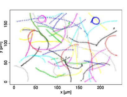
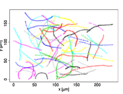
Figure 1: All bacterial trajectories recorded in medium 0 (no nutrients) at times $t_{0}$=0min in (top, 54 trajectories) and $t_{\mathrm{end}}$=84min (bottom, 61 trajectories). At both times, the movie length evaluated was about 17 sec with a time resolution of 0.11 sec, i.e. about 700 frames per movie. The points of the trajectories show 26 of these frames. The rectangular boundaries are a consequence of the camera calibration.

Given the trajectories measured at a time resolution of 0.11 sec, we are able to calculate the velocity vector in the two-dimensional space as

$$\mbox{\boldmath$v$}^{k}_{t_{j}}=\frac{\mbox{\boldmath$r$}^{k}_{t_{j}}-\mbox{\boldmath$r$}^{k}_{t_{j-1}}}{t_{j}-t_{j-1}}$$ (14)

where $k$ denotes the bacterial cell and $j$ refers to the time step. The velocity distributions are shown in Fig. 2 both for the initial situation (blue dots at $t_{0}$) and after a sufficient long time of relaxation (red dots at $t_{\mathrm{end}}$) and for the three different media used. Each of the samples contains about 1.500 data points.

In all cases, we observe the formation of rings of different radii, indicating that bacteria swim at comparable velocities in the time intervals of observation and that their motion is isotropic, i.e. that they do not have a preferrred direction of motion. Most interesting, compared to the initial distribution the rings either contract (medium 0) or expand (medium 1, 2) in diameter, which means that the bacteria have adjusted their individual velocities according to the nutrient concentration available. This will be systematically investigated in the next section. The available data do not allow us to predict if the rings completely contract (medium 0) or further expand (medium 1,2 ) their extension.

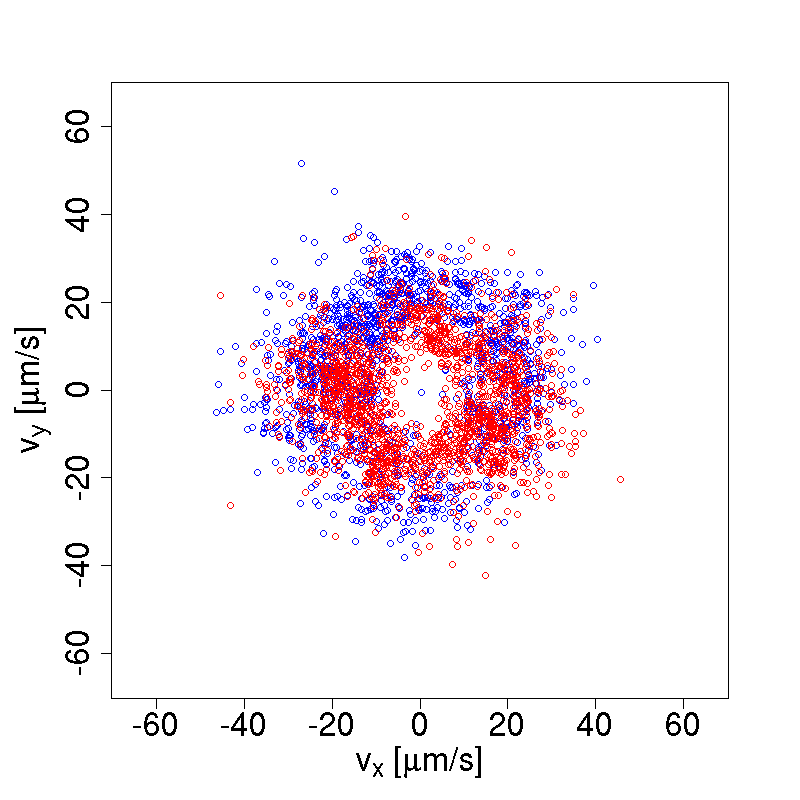
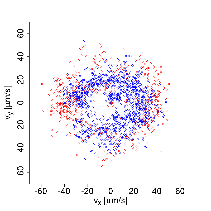
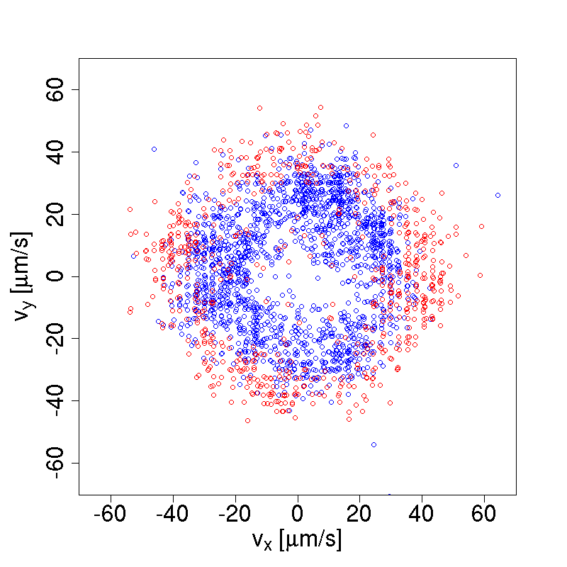
Figure 2: Snapshots of the two-dimensional velocity distributions around times $t_{0}$ (blue dots) and $t_{\mathrm{end}}$ (red dots), shown for the three different media: (left) medium 0, (middle) medium 1, (right) medium 2. Each of the samples contains about 1.500 data points.

4 Investigating the velocity distribution

4.1 The Fokker-Planck Perspective

The experiments described above have clearly shown that bacteria adjust their velocity dependent on the nutrient available in the medium. It remains (i) to quantify this influence, and (ii) to compare the outcome with the hypothesis made on the velocity dependent transfer of internal energy. Such a comparison cannot be made on the level of individual trajectories, but only on the level of the ensemble average.

Hence, in the following we use the two-dimensional velocity distribution $p(\mathbf{v},t)$, which follows a Fokker-Planck equation [11, 24] that corresponds to the Langevin eqn. 6):

$$\frac{\partial p(\mbox{\boldmath$v$},t)}{\partial t}=\mbox{\boldmath$\nabla$}_{v}\left[\gamma\mathbf{v}\left(1-\frac{q_{0}}{\gamma_{0}}\frac{d(v)}{\left[c+d(v)\right]\mbox{\boldmath$v$}^{2}}\right)\mbox{\boldmath$v$}\;p(\mbox{\boldmath$v$},t)+S~{}\mbox{\boldmath$\nabla$}_{v}p(\mbox{\boldmath$v$},t)\right]$$ (15)

This Fokker-Planck equation is based on the assumption that the internal energy depot has reached a quasistationary equilibrium fast enough. If we assume the general hypothesis $d(v)=d_{2}{v}^{\xi}$ and $\dot{p}=0$, we find for the stationary velocity distribution

$$p^{0}(\mbox{\boldmath$v$})=C\left(1+\frac{d_{2}{v}^{\xi}}{c}\right)^{\frac{q_{0}}{\xi mS}}\exp\left(-\frac{\gamma}{2S}\mbox{\boldmath$v$}^{2}\right),$$ (16)

where the normalization condition $C$ is defined through the condition $1=\iint p^{0}(\mbox{\boldmath$v$})d\mbox{\boldmath$v$}$. For $\xi=2$ the SET model results and the stationary solution, eqn. (16), can be written in first-order expansion as:

$$p^{0}(\mbox{\boldmath$v$})\sim\exp\left(-\frac{\gamma}{2S}\left[1-Q_{2}\right]\mbox{\boldmath$v$}^{2}+\cdots\right)$$ (17)

As has been discussed in detail [11], for $Q_{2}<1$ we find a unimodal Maxwell-like velocity distribution, whereas for $Q_{2}>1$ a crater-like velocity distribution results in two-dimensional systems.

The amount of data measured does not allow us to reasonably reconstruct the two-dimensional velocity distribution by means of density approximations. Therefore, in the following, we restrict ourselves to the distribution of the speed which contains sufficient information to test our hypotheses given. To find the speed distribution $p^{0}_{a}(v)$ in two dimensions we integrate over a disk $B(v^{\prime})$:

$$P^{0}(|\mbox{\boldmath$v$}|<v^{\prime})=\iint_{B(v^{\prime})}p^{0}(\mbox{\boldmath$v$})dv_{x}dv_{y}=2\pi\int_{0}^{v^{\prime}}p^{0}(v)dv=\int_{0}^{v^{\prime}}p^{0}_{a}(v)dv$$ (18)

and find

$$p^{0}_{a}(v)=C_{a}2\pi v\left(1+\frac{d_{2}{v}^{\xi}}{c}\right)^{\frac{q_{0}}{\xi mS}}\exp\left(-\frac{\gamma}{2S}v^{2}\right)$$ (19)

When comparing this equation with eqn. 16, one should note the additional prefactor $v$. So, for the maximum of $p_{a}^{0}(v)$, instead of the compact expression (12) resulting from ${p}^{0}(\mathbf{v})$, we find a rather intricate expression which is not reprinted here. Instead, the stationary speed distribution is plotted in Fig. 3 for the SET model and different values of $Q_{2}$. Different from the noticable change between unimodal and crater-like shape of the stationary velocity distribution $p^{0}(\mathbf{v})$, we observe only a shift in the maximum of $p_{a}^{0}(v)$ when $Q_{2}$ changes from subcritical to supercritical values. At second view, one notices that the ascent of $p_{a}^{0}(v)$ changes from a linear increase for $Q_{2}<1$ to an nonlinear increase $v^{n}$ for $Q_{2}>1$, where $n$ is an integer.

Figure 3: $p_{a}^{0}(v)$, eqn. (19), for $\xi=2$ and different values of $Q_{2}$: (blue) $Q_{2}=0.35$, (green) $Q_{2}=1$, (red) $Q_{2}=3.5$. The speed $v$ is given in abitrary units.

Specifically, we do not need to explicitely derive the maximum of the speed distribution (which is also known as the most probable value and different from, e.g., the expecation value or the average value), because we want to compare the theoretical and the experimental distributions $p_{a}(v)$ rather than their extreme values. These distributions, in addition to their mean value, are further characterized by their width, given by the variance $\sigma^{2}=S/\gamma$. Hence, we need to determine the strength $S$ of the stochastic force in relation to the friction coefficient $\gamma$.

4.2 Determining the noise intensity

In statistical physics, the strength of the stochastic force is related to the thermal velocity of microscopic particles, e.g. molecules or Brownian particles, via the fluctuation-dissipation theorem, which yields for ideal gases $S/\gamma=k_{B}T/m$, where $k_{B}$ is the Boltzmann constant. If one wishes to apply the same relation also to bacteria like Escherichia coli or Salmonella typhimurium at about $T=300$, with a bacterial mass of $m\approx 10^{-15}$, one arrives at $\sigma=2000\mu$m/s, which about two orders of magnitude larger than the average velocity for such bacteria. Given the rather complex nature of bacterial motion described above, this discrepancy is not really surprising.

Therefore, in [21] a different method to determine $S/\gamma$ was proposed, which is based on the speed autocorrelation function

$$g_{v}(\tau)=\frac{\left\langle v(t_{1})v(t_{2})\right\rangle}{\left\langle v(t_{1})v(t_{1})\right\rangle}\;;\quad\tau=\left|t_{2}-t_{1}\right|$$ (20)

The calculation of $g_{v}(\tau)$ needs a formal solution of the Langevin equation for the speed ${v}(t)$. This was provided in [21] for a different model applied to the migration of human granulocytes. It postulates a stationary speed $v_{s}$ and assumes, different from our ansatz of eqn. (6),

$$\dot{{v}}_{i}=-\gamma{v}_{i}\left[1-\frac{v_{s}}{v}\right]+\sqrt{2S}\ {\xi}_{i}(t)$$ (21)

It was noted that in this equation an additive Gaussian random noise is physically and mathematically problematic as it allows in principle negative speed values. As possible solution, one can consider appriopriate boundary conditions or a different definition of the velocity-dependent friction term as suggested recently [19]

In the following, we still use eqn. 21, but point out that this is only an approximation in the limit of small noise with respect to the finite stationary speed. The stationary solution for the speed autocorrelation function is reached when the times $t_{1}$ and $t_{2}$ are larger than the characteristic time $\gamma^{-{1}}$, which results into

$$\left\langle v(t_{1})v(t_{2})\right\rangle=v_{s}^{2}+\frac{S}{\gamma}\exp\left\{-\gamma|t_{2}-t_{1}|\right\}$$ (22)

In the limit $\tau\to\infty$, the speed autocorrelation function $g_{v}(\tau)$ becomes a constant, $g_{v}={v_{s}^{2}}/[{v_{s}^{2}+{S}/{\gamma}}]$, which can be measured experimentally, to obtain:

$$\sigma^{2}=\frac{S}{\gamma}=v_{s}^{2}\left(\frac{1-g_{v}}{g_{v}}\right)$$ (23)

Schienbein and Gruler [21] found for human granulocytes, which are much larger than the bacterial cells investigated here, $g_{v}=0.82$ and from the measured speed distribution the maximum value $v_{s}=17\mu$m/min.

As mentioned, our Langevin equation uses a different ansatz for the velocity-dependent friction function, which does not allow us to obtain a simple closed form for $g_{v}$. However, we can still apply the results of [21] arguing that the speed of bacteria in the stationary limit reaches values around $v_{s}$. Hence, in the vicinity of $v_{s}$, we linearize the dependence on $v$, which is $1/v^{2}$, to $1/v$ and use for $v_{s}$ the expression given by eqn. (12) for the SET model, or by eqn. (13) for $1<\xi<2$. This approximation allows us to use eqn. (23) to determine $S/\gamma$ provided we can obtain $v_{s}$ and $g_{v}$ from our own experiments.

4.3 Parameter Estimation

With these considerations, we have all ingredients together to compare our experimental data with the theoretical predictions. In detail. we proceed as follows:

1. For the three media described above (Sect. 3.1), we calculate the absolute velocities $v_{aj}^{k}$ of each cell $k$ tracked during the time step $j$. For each medium, two measurements were taken: (a) initially, time $t_{0}$, (b) after sufficiently long time, about one hour, time $t_{end}$ (see also Fig. 2 for the two-dimensional velocity distributions). From these samples, which contain about 1.500 data points each, we calculate the densities $p_{a}^{\mathrm{exp}}(v)$ using the Sheather-Jones method of selecting a smoothing parameter for density estimation [26] in R. The results are shown by the blue curves in Fig. 4 for $t_{\mathrm{end}}$.

2. From the 6 different density plots, we calculate the maximum $v_{s}$ of the experimental speed distribution $p_{a}^{\mathrm{exp}}(v)$. The results are given in Appendix C: Table 1. For $t_{\mathrm{end}}$, we also calculate the speed autocorrelation function $g_{v}$, which is shown in Table 1 as well.

3. Eventually, we apply the maximum-likelihood estimation (MLE) to find out, which of the still undertermined parameters fit best the experimental densities $p_{a}^{\mathrm{exp}}(v)$. The parameter details are presented in Appendix C: Table 2, while the resulting density plots for the hypotheses $\xi=2$ and $1<\xi<2$ are shown by the red curves in Fig. 4, which are to be compared with the experimental findings (blue curves).

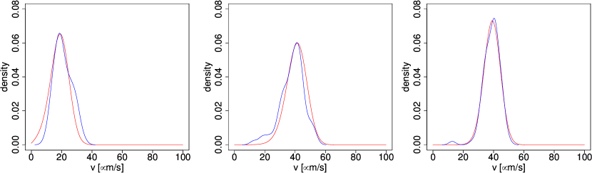
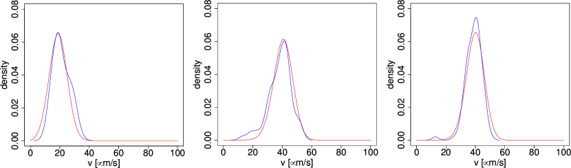
Figure 4: (blue curves) Estimated densities $p_{a}^{\mathrm{exp}}(v)$ obtained from experimental measurements of the speed (absolute velocity) $v$ $[\mu$m/s] at time $t_{\mathrm{end}}$. (red curves) Calculated densities $p_{a}(v)$, eqn. (19) using the parameters of the MLE, Table 2. (top row) SET model with $\xi=2$, (bottom row) $1<\xi<2$. (left figures) medium 0, (middle figures) medium 1, (right figures) medium 2.

In the following, we further discuss these findings. In Table 1, one notes slight differences in $v_{s}(t_{0})$ for the different media. This indicates that at time $t_{0}$, right after being put into the medium, the bacterial cells already started to adjust to the nutrient concentration in the media. The higher the concentration, the higher $v_{s}$. This can be also confirmed at $t_{\mathrm{end}}$, after about 80 min. The differences between medium 1 and 2 (middle and high concentration) is rather small both for at $t_{0}$ and $t_{\mathrm{end}}$, indicating that there seems to be a saturation in converting internal into kinetic energy. This saturation can be caused by intracellular processes (e.g. number of receptor proteins available), but is not further discussed here. Noticable, in medium 0 (no nutrients), $v_{s}$ drops down considerably compared to the initial value, which also indicates that the bacterial cells respond to the available energy by adjusting their speed.

We further find that the speed autocorrelation function $g_{v}$ returns comparable values for all three media ($0.92-0.98$) which are much larger than for granulocytes, because we have much smaller and more motile cells. The estimated standard deviations $\sigma=\sqrt{S/\gamma}$ range between $5.49\mu$m/s (medium 0) and $5.83\mu$m/s (medium 2) and are quite similar for all media, because the temperature and the viscosity of the media are kept as constant as possible.

The actual width of the speed distribution, however, does not just depend on $S/\gamma$ but also on the parameters of the internal energy depot and is therefore larger than $\sigma$. In order to calculate the parameter values that maximize the likelihood, we restrict ourselves to reduced parameters. Keeping in mind that $\sigma^{2}=S/\gamma$ is given by eqn. (23) and the control parameter is defined as $Q_{2}=(q_{0}d_{2})/(\gamma mc)$, we can rewrite the leading terms in eqn. (19) as:

$$\left(1+\frac{d_{2}{v}^{\xi}}{c}\right)^{\frac{q_{0}}{\xi mS}}\exp\left(-\frac{\gamma}{2S}v^{2}\right)=\left(1+\frac{d_{2}}{c}{v}^{\xi}\right)^{\frac{Q_{2}}{\xi\sigma^{2}}\frac{c}{d_{2}}}\exp\left(-\frac{v^{2}}{2\sigma^{2}}\right)$$ (24)

which reduces the number of parameters to be determined to $(d_{2}/c)$ and $Q_{2}$, while $\sigma^{2}$ is given by the experiments. $\xi$ on the other hand is either set to 2, in case of the SET model, or used as a free parameter. Given the observations $v_{1},v_{2},...,v_{n}$ the MLE then determines for which values $\Theta$ of these parameters the likelihood function $L(v_{1},v_{2},...,v_{n},\Theta)$ is maximised, i.e. what are the most likely model parameters that fit the experimental data best, conditional on the model used.

In order to fully appreciate the MLE, we have to notice that no further “logical” assumption are made, i.e., each for experimental distribution the MLE returns that set of parameter values that fits this particular distribution best. Precisely, we receive most likely a different set of values for each of the given distributions. To put it the other way round, from all the observed distributions we can obtain a range of parameter values that is compatible with the experimental findings, rather than a precise value that is met by all observations.

With this in mind, we can interpret Table 2 as follows: For both hypotheses, the SET model with $\xi=2$ and the general model with $1<\xi<2$, we find from the observations a “reasonable” (but different) set of parameters that supports these hypotheses. This is also confirmed by the fits shows in Figure 4. I.e., we cannot reject one of these hypotheses as they both match the experimental findings. However, we did not observe a subciritical take-up of energy for the SET model, as we did not find values $Q_{2}<1$ for the given observations. The latter conclusion needs a further explanation: In medium 0, we made no nutrients available, so $q_{0}$ and $Q_{2}$ should both be zero. However, the bacteria were grown in a medium that contained nutrients and thus, at time $t_{0}$, started their motion with a filled energy depot $e^{\mathrm{st}}$, eqn. (3), that changes over time only rather slowly as $v_{s}$ is adjusted. Hence, the value $Q_{2}$ for medium 0 at time $t_{\mathrm{end}}$ reflects the value of the internal energy depot at time $t_{\mathrm{end}}$. As the observations in Figures 2, 4 and Table 1 show, even after a long time the bacteria still have energy enough to move with a non-trivial speed $v_{s}$ despite the fact that no nutrients are provided. But there is a clear trend toward slowing down as the values indicate.

As second interesting observation regards the decrease of the $d_{2}/c$ values with increasing nutrient concentration (comparing medium 1 and 2), for both the SET and the $\xi$ model. The ratio $M=d_{2}v_{s}^{2}/c$ reflects the proportion of energy bacteria spend on the two different processes, active motion and metabolism. If more energy becomes available (from medium 1 to 2) , this does not necessarily lead to a speed-up – the speed was kept almost constant, but the additional energy is likely spent on metabolism (and growth). Hence $M$ decreases from 1.50 to 0.62 for the SET model, and from 0.74 to 0.23 for the $\xi$ model, while the take-up of energy $q_{0}/\gamma_{0}$ has increased from 2500 to 4140 for the SET model, and from 5230 to 6800 for the $\xi$ model. So, in conclusion, our model suggests that bacteria indeed take up more energy from the environment if more nutrients are provided, but the ratio spent on active motion is decreased, while the ratio spent on metabolism is increased.

5 Conclusions

The aim of this paper is twofold: (i) we investigate to what extent a theoretical model of active motion, namely that of “active Brownian particles”, is compatible with experimental findings from bacterial cell motility, (ii) we test the impact of available energy in the environment, varied by the nutrient concentration in the medium, on the speed distribution of bacterial cells.

For the discussion one has to keep in mind that our results have been obtained for a particular strain of Salmonella typhimurium (see Sect. 3.1. and Appendix A) and cannot easily generalized to other bacterial cells. This is because of the rather complex cellular motion of bacteria which, in many cases, is comprised of tumbling and nontumbling phases (see Sect. 3.1). Hence, for the motion of other types of bacteria we refer to the extensive literature [14, 27, 2, 16, 3, 13, 18, 15, 12].

Comparing the experiments with moving S. typhimurium and the theoretical model, we demonstrated that the measured speed distribution can indeed be matched by the analytical prediction. This holds for both tested hypothesis, (a) the SET model with $\xi=2$ and (b) the $\xi$ model, which allows an adjustment of the exponent, $1<\xi<2$. We further confirmed that, under the give experimental conditions, bacteria move in the supercritical regime, $Q_{2}>1$. However, we were not able to observe as subcritical behavior with $Q_{2}<1$ as predicted for the SET model [10, 8]. This can be probably explained by the fact that even at the end of our experiments bacterial cells had still enough internal energy available from their growing period, to move with a nontrivial speed. But we could notice a considerable slowing down of 25 with no additional nutrients.

Regarding the impact of available nutrients, we found that the speed of bacteria did not increase in proportion to it. Instead, we observed a more or less constant speed, even if the nutrient concentration was doubled. From calculating the model parameters for both cases, we conjecture that indeed more energy was taken up by the cells, but this was used for other internal processes such as metabolism and growth.

In conclusion, the experiments carried out with bacterial cells moving in media of three different nutrient concentrations could confirm the theoretical predictions and thus indirectly also support the assumptions made for our model of active Brownian particles. However, particular details of the choice of parameters cannot be fully resolved by our experiments – which is not very surprising. This regards for example the “correct” value of the exponent $\xi$ for the speed, $v^{\xi}$. Our findings support values between 1.67 and 2.0 if a take-up of energy from the medium was possible. The differences between the two assumptions are not so much in the values of $\xi$ but in the theoretical consequences. In the case of the SET model, there is a clear bifurcation which allows to distinguish between subcritical (Brownian motion like) behavior, and supercritical behavior characterized by a directed motion. It would still be interesting to find microorganisms for which these regimes could be determined. Our experiments had to restrict to the conditions explained above and therefore do not support this distinction.

Appendix A: Details of Bacterial Probes

The chemotaxis-deficient Salmonella strain M935 (SL1344; cheY::Tn10, [29, 31]) was grown under mild aeration for 12 h/37^∘C in LB medium containing 0.3 M NaCL. The culture was diluted 1:20 into fresh medium and grown for another 4h / 37^∘C. Bacteria were pelleted by centrifugation (8500 rpm, 5 min, 4^∘C) and resuspended in phosphate-buffered saline (PBS). The sample was centrifuged again and the bacteria were resuspended either in PBS (probe A) or LB medium (probe B). From these two probes, samples for live imaging of the bacteria were prepared as follows:

1. probe A was diluted 1:50 in PBS containing 5 (BSA) and transferred to a glass-bottom dish for imaging

2. a glass-bottom dish was rinsed with PBS/5 of bacteria to the glass surface. PBS/BSA was removed and a 1:50 dilution of probe B in LB was added to the dish for imaging

3. probe B was diluted 1:50 in a 1:1 mixture of PBS/5 (final BSA concentration: 2.5

All solutions for dilution of probes A and B were prewarmed to 37^∘C.

Appendix B: Details of Data Evaluation

For time lapse microscopy the different samples were mounted onto a heated specimen holder (37^∘C) on a Zeiss Asiovert 200m inverted microscope. Time series of phase contrast images were recorded using a Plan Neofluoar 20x (NA 0.5) objective at a rate of ca. 20 images per second.

Motile bacteria were tracked using Particle tracker software [20] as plugin on the pure Java image processing program ImageJ [1]. Only trajectories appearing over more than 30 time frames were considered. Selected trajectories were manually verified for correct tracking (Wrong tracking occurred in cases of crossings between identified bacteria and was removed from the trajectories). These criteria for track evaluation were equally applied on all detected trajectories. About 3 hours of eye selection are necessary to obtain about fifteen to twenty tracks. The evaluation of the data was carried out by an R-script written by the authors.

Appendix C: Details of Parameters Obtained

Medium	$v_{s}(t_{0})$ [$\mu$m/s]	$v_{s}(t_{\mathrm{end}})$ [$\mu$m/s]	$g_{v}(t_{\mathrm{end}})$
0	24.2	19.8	0.920
1	27.8	38.8	0.979
2	29.3	39.5	0.981

Table 1: Maxima $v_{s}$ (10^-6 m/s) of the experimental speed distribution $p_{a}^{\mathrm{exp}}(v)$ taken initially ($t_{0}$) and after long time ($t_{\mathrm{end}}$) for 3 different media (see Sect. 3.1). $g_{v}(t_{\mathrm{end}})$ gives the value of the speed autocorrelation function measured experimentally at time $t_{\mathrm{end}}$.

Medium	${d_{2}}/{c}$ [(s$/(\mu$m$)^{2}$]	$Q_{2}$	${}^{\star}{d_{2}}/{c}^{\star}$ [(s$/(\mu$m$)^{2}$]	${}^{\star}Q_{2}^{\star}$	$\xi$
0	$2.3\cdot 10^{-3}$	1.75	$33.3\cdot 10^{-4}$	8.50	1.52
1	$1.0\cdot 10^{-3}$	2.63	$\;\;9.5\cdot 10^{-4}$	4.97	1.82
2	$0.4\cdot 10^{-3}$	1.70	$\;\;5.1\cdot 10^{-4}$	3.47	1.67

Table 2: Parameter values of $p_{a}(v)$, eqn. (19), as estimated by MLE for the SET model, $\xi=2$ (no-starred values) and for the general model, $1<\xi<2$ (starred values) at time $t_{\mathrm{end}}$.

Acknowledgment

The authors are deeply indebted to Wolf-Dietrich Hardt for providing access to, and use of, his laboratory at the Institute of Microbiology of ETH Zurich, where V.G. could carry out the experiments. We further gratefully acknowledge scientific discussions with Howard C. Berg, Wolf-Dietrich Hardt and Markus C. Schlumberger.

References

- Abramoff et al. [2004] Abramoff, M.; Magelhaes, P.; Ram, S. (2004). Image processing with ImageJ. Biophotonics Int 11(7), 36–42.
- Berg [2003] Berg, H. (2003). The rotary motor of bacterial flagella. Annu Rev Biochem 72, 19–54.
- Berry and Armitage [1999] Berry, R.; Armitage, J. (1999). The bacterial flagellar motor. Adv. Microb. Physiol 41, 291–337.
- Birbaumer and Schweitzer [2011] Birbaumer, M.; Schweitzer, F. (2011). Agent-Based Modeling of Intracellular Transport. European Physical Journal B 82(3-4), 245–255.
- Chen and Berg [2000] Chen, X.; Berg, H. (2000). Torque-Speed Relationship of the Flagellar Rotary Motor of Escherichia coli. Biophysical Journal 78(2), 1036–1041.
- Condat et al. [2005] Condat, C.; Jäckle, J.; Menchón, S. (2005). Randomly curved runs interrupted by tumbling: A model for bacterial motion. Physical Review E 72(2), 21909.
- Condat and Sibona [2002a] Condat, C.; Sibona, G. (2002a). Diffusion in a model for active Brownian motion. Physica D: Nonlinear Phenomena 168, 235–243.
- Condat and Sibona [2002b] Condat, C.; Sibona, G. (2002b). Noise-enhanced mechanical efficiency in microorganism transport. Physica A: Statistical Mechanics and its Applications 316(1-4), 203–212.
- Ebeling and Schweitzer [2003] Ebeling, W.; Schweitzer, F. (2003). Self-organization, active Brownian dynamics, and biological applications. Nova Acta Leopoldina NF 88(332), 169–188.
- Ebeling et al. [1999] Ebeling, W.; Schweitzer, F.; Tilch, B. (1999). Active Brownian particles with energy depots modeling animal mobility. BioSystems 49(1), 17–29.
- Erdmann et al. [2000] Erdmann, U.; Ebeling, W.; Schimansky-Geier, L.; Schweitzer, F. (2000). Brownian particles far from equilibrium. The European Physical Journal B-Condensed Matter 15(1), 105–113.
- Greenberg and Canale-Parola [1977] Greenberg, E.; Canale-Parola, E. (1977). Motility of flagellated bacteria in viscous environments. Journal of Bacteriology 132(1), 356.
- Levin et al. [1998] Levin, M.; Morton-Firth, C.; Abouhamad, W.; Bourret, R.; Bray, D. (1998). Origins of Individual Swimming Behavior in Bacteria. Biophysical Journal 74(1), 175–181.
- Liao et al. [2007] Liao, Q.; Subramanian, G.; DeLisa, M.; Koch, D.; Wu, M. (2007). Pair velocity correlations among swimming Escherichia coli bacteria are determined by force-quadrupole hydrodynamic interactions. Physics of Fluids 19, 061701.
- Lowe et al. [1987] Lowe, G.; Meister, M.; Berg, H. (1987). Rapid rotation of flagellar bundles in swimming bacteria. Nature 325(6105), 637–640.
- Magariyama et al. [2001] Magariyama, Y.; Sugiyama, S.; Kudo, S. (2001). Bacterial swimming speed and rotation rate of bundled flagella. FEMS Microbiology Letters 199(1), 125–129.
- Manson et al. [1980] Manson, M.; Tedesco, P.; Berg, H. (1980). Energetics of flagellar rotation in bacteria. J Mol Biol 138(3), 541–61.
- Mitchell [1991] Mitchell, J. (1991). The influence of cell size on marine bacterial motility and energetics. Microbial Ecology 22(1), 227–238.
- Romanczuk and Schimansky-Geier [2011] Romanczuk, P.; Schimansky-Geier, L. (2011). Brownian Motion with Active Fluctuations. Phys. Rev. Lett. 106(23), 230601.
- Sbalzarini and Koumoutsakos [2005] Sbalzarini, I.; Koumoutsakos, P. (2005). Feature point tracking and trajectory analysis for video imaging in cell biology. Journal of Structural Biology 151(2), 182–195.
- Schienbein and Gruler [1993] Schienbein, M.; Gruler, H. (1993). Langevin equation, Fokker-Planck equation and cell migration. Bulletin of Mathematical Biology 55(3), 585–608.
- Schweitzer [2003] Schweitzer, F. (2003). Brownian Agents and Active Particles: Collective Dynamics in the Natural and Social Sciences. Springer.
- Schweitzer et al. [1998] Schweitzer, F.; Ebeling, W.; Tilch, B. (1998). Complex Motion of Brownian Particles with Energy Depots. Physical Review Letters 80(23), 5044–5047.
- Schweitzer et al. [2001] Schweitzer, F.; Ebeling, W.; Tilch, B. (2001). Statistical mechanics of canonical-dissipative systems and applications to swarm dynamics. Physical Review E 64(2), 21110.
- Schweitzer and Tilch [2002] Schweitzer, F.; Tilch, B. (2002). Self-assembling of networks in an agent-based model. Physical Review E 66(2), 026113.
- Sheather and Jones [1991] Sheather, S.; Jones, M. (1991). A reliable data-based bandwidth selection method for kernel density estimation. J. Roy. Statist. Soc. Ser. B 53(3), 683–690.
- Sherwood et al. [2003] Sherwood, J.; Sung, J.; Ford, R.; Fernandez, E.; Maneval, J.; Smith, J. (2003). Analysis of Bacterial Random Motility in a Porous Medium Using Magnetic Resonance Imaging and Immunomagnetic Labeling. Environmental Science & Technology 37(4), 781–785.
- Sibona [2007] Sibona, G. (2007). Evolution of microorganism locomotion induced by starvation. Physical Review E 76(1), 11919.
- Stecher et al. [2008] Stecher, B.; Barthel, M.; Schlumberger, M.; Haberli, L.; Rabsch, W.; Kremer, M.; Hardt, W. (2008). Motility allows S. Typhimurium to benefit from the mucosal defence. Cellular microbiology 10(5), 1166–1180.
- Steuernagel et al. [1994] Steuernagel, O.; Ebeling, W.; Calenbuhr, V. (1994). An Elementary Model for Directed Active Motion. Chaos, Solitons & Fractals 4, 1917–1930.
- Winnen et al. [2008] Winnen, B.; Schlumberger, M.; Sturm, A.; Schüpbach, K.; Siebenmann, S.; Jenny, P.; Hardt, W. (2008). Hierarchical Effector Protein Transport by the Salmonella Typhimurium SPI-1 Type III Secretion System. PLoS ONE 3(5).