Measurements of Spin Correlation in $t\bar{t}$ Events at D0

Abstract

Two recent measurements by the D0 Collaboration of spin correlation in $t\bar{t}$ production using 5.4 fb^-1 of Tevatron $p\bar{p}$ collider data are presented. Both rely on the dilepton final state of $t\bar{t}$. One measurement relies on full reconstruction of the top quark kinematics, and the other makes use of leading-order matrix elements to characterize the kinematics. The latter measurement is the first ever to have sufficient analyzing power to exclude the no-correlation hypothesis.

I Introduction

In the $p\bar{p}\to q\bar{q}$ process, the quarks that are produced are unpolarized, but their spins are correlated. This is required by angular momentum conservation in the strong interaction. In general, this correlation is unobservable, as the hadronization process involves the emission of gluons that can flip the spins of the quarks. But the top quark provides a laboratory for studying the correlation. The short lifetime of top, about $5\times 10^{-25}$ s, is shorter than the timescale for strong processes, so top decays before fragmentation and spin flips can occur. Thus, the original spin orientation is preserved, and is passed to the decay products. It should then be observable through a study of the kinematics of the decay products.

A measurement of top-quark spin correlation is a test of top-quark properties and also a probe of new physics. The very observation of the correlation could in principle be used to set an upper limit on the top lifetime. Should top have a non-standard decay (such as $t\to H^{+}b$), or non-standard production mechanism (through decays of stop pairs, or a $Z^{\prime}$ resonance), a non-standard correlation would be observed. The correlation is ultimately a subtle effect – the theme of this presentation – but there is now enough Tevatron data to explore it.

II About correlation

At the Tevatron, the primary production mode of $t\bar{t}$ is through $q\bar{q}\to t\bar{t}$ with an $s$-channel gluon. (This is in contrast to the LHC, where the initial state is primarily $gg$). The $q$ and $\bar{q}$ must have opposite helicity to couple to that gluon, and that forces the $t$ and $\bar{t}$ to have their spins pointing along the beamline. A correlation strength can be defined based on the number of $t\bar{t}$ pairs with their spins pointing in the same direction,

$$A=\frac{N_{\uparrow\uparrow}+N_{\downarrow\downarrow}-N_{\uparrow\downarrow}-N_{\downarrow\uparrow}}{N_{\uparrow\uparrow}+N_{\downarrow\downarrow}+N_{\uparrow\downarrow}+N_{\downarrow\uparrow}}.$$ (1)

But the spin orientation must be defined with respect to a quantization axis. In the measurements described here, the beamline axis, defined as the direction of the colliding hadrons in the zero-momentum frame of the $t\bar{t}$ system, is used. This choice is intuitive, easy to construct, and optimal for $t\bar{t}$ produced at threshold. With this choice of quantization axis, next-to-leading order QCD calculations predict $A=0.777^{+0.027}_{-0.042}$ bib:Avalue .

The spin orientation of the top is then passed to its decay products. The differential angular decay distributions of the top daughters is given by

$$\frac{1}{\Gamma}\frac{d\Gamma}{d\cos\theta_{i}}=\frac{1}{2}(1+\alpha_{i}\cos\theta_{i}),$$ (2)

where $\cos\theta_{i}$ is the angle between the $i$th top daughter and the spin of the top. Different decay products have different correlation strengths, as indicated by $\alpha_{i}$. This is illustrated in Figure 1. In the case of a leptonic $W$ decay, the lepton has the greatest analyzing power, and for a hadronic $W$ decay it is the down-type quark. In both cases, $\alpha\simeq 1$.

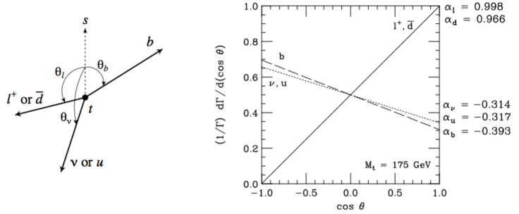
Figure 1: Illustration of the top decay angles (left) and dependence of the decay rate on the angles (right) bib:mahlon .

Thus, the doubly-differential cross section as a function of the decay angles of decay products from two different quarks in $t\bar{t}$ is given by

$$\frac{1}{\sigma}\frac{d^{2}\sigma}{d\cos\theta_{1}d\cos\theta_{2}}=\frac{1}{4}(1-A\alpha_{1}\alpha_{2}\cos\theta_{1}\cos\theta_{2}).$$ (3)

To study the spin correlation, one looks for correlation between the directions of decay products from the two different top decays. In the case of both tops decaying leptonically, $\alpha_{1}\alpha_{1}\simeq 1$, and we write $A\alpha_{1}\alpha_{2}\equiv C\simeq A$.

III Experimental situation

The measurements described below were performed at the Fermilab Tevatron, a $p\bar{p}$ collider operating at $\sqrt{s}=1.96$ TeV. Run II of the collider has been in progress since 2001, with almost 12 fb^-1 of integrated luminosity delivered. The spin-correlation measurements make use of 5.4 fb^-1. The data was recorded by the D0 detector, which consists of silicon and fiber trackers inside a 2 T solenoid, a liquid argon-uranium calorimeter, and muon trackers and scintillators inside toroids.

At the Tevatron, 85% of $t\bar{t}$ production arises from $q\bar{q}$ annihilation and the remaining 15% from $gg$ interactions. Each top quark decays to $Wb$ nearly 100% of the time, and the final states are characterized by the $W$ decay modes. The three final states are all-hadronic, lepton plus jets and dilepton. In the order listed, the final states have decreasing rate and increasing number of neutrinos and signal purity.

The dilepton state in particular is characterized by two high-$p_{T}$ leptons, missing momentum due to the escaping neutrinos, two hadronic jets from $b$ decays, and perhaps additional jets due to initial- and final-state radiation. For the purpose of the spin-correlation measurements, the dilepton state has the best analyzing power and most accurate measurement of the decay-product (lepton) directions, but the worst statistical power, compared to other final states that could be considered.

IV Event selection

The two measurements described have the same event selection. A $t\bar{t}$-enriched sample is chosen by selecting events with two high-$p_{T}$, isolated, opposite-charge leptons. Only electrons and muons are considered as leptons, so the dilepton pairs can be either $ee$, $e\mu$ or $\mu\mu$.. There must also be at least two high-$p_{T}$ jets. To suppress backgrounds, a large scalar sum of the lepton and jet $p_{T}$ values is required in the $e\mu$ channel, and significant missing energy in the $ee$ and $\mu\mu$ channels. Backgrounds from $Z/\gamma^{*}$ (diboson) events are modeled by leading-order Monte Carlo samples, and normalized to next-to-next-to-leading (next-to-leading) order cross sections. Instrumental backgrounds arise from misidentified $\pi^{0}$ and $\eta$ decays in electron samples and real muons in jets that appear to be isolated in muon samples; both of these are modeled with complementary data samples. The selected data sample is about 70% pure in $t\bar{t}$ events, as shown in Table 1.

Table 1: Estimates of contributions of various physics processes to the selected dilepton sample.

$t\bar{t}$	$Z/\gamma^{*}$	Diboson	Instrumental	Total	Observed
$341\pm 30$	$93\pm 15$	$19\pm 3$	$28\pm 5$	$481\pm 39$	485

V Analysis I: Template-based

D0 has performed two different measurements of the spin correlation with this event sample. The first is template-based, in which the decay angles are calculated in each event, and the distribution of angles is modeled by a sum of templates representing the distributions for correlated and uncorrelated spins bib:meas1 . This technique has been used before bib:old1 , but with a much smaller data sample.

To observe the correlation, one must measure the angle between the lepton and the beamline (which is used as the top spin quantization axis) in the zero-momentum frame of the $t\bar{t}$ system, which requires a full reconstruction of the decay. A total of eighteen quantities are needed to specify the final-state configuration, but because of the two undetected neutrinos only twelve are measured. Constraining the decay kinematics to the values of the top and $W$ masses provides four additional pieces of information, but that still leaves two missing.

The “neutrino weighting” technique is used to solve the remaining kinematics. Two values of the neutrino $\eta$ (where $\eta=-\ln\tan(\theta/2)$ and $\theta$ is the polar angle measured from the beamline) are randomly sampled from the neutrino $\eta$ distribution as predicted from $t\bar{t}$ Monte Carlo simulations. These values are then used to solve for the implied $t\bar{t}$ kinematics. This allows a determination of the product of decay angles $\cos\theta_{1}\cos\theta_{2}$ and of the neutrino momenta. The $\cos\theta_{1}\cos\theta_{2}$ value is then weighted by the consistency of the determined neutrino momenta with the measured missing transverse energy in the event. The sampling is repeated many times, and weighted mean of all solutions obtained is then used as the estimator of $\cos\theta_{1}\cos\theta_{2}$.

$t\bar{t}$ events are simulated using the MC@NLO generator bib:MCNLO , in which the spin correlation can be turned on or off straightforwardly. Then, with the appropriate weighting of simulated samples, $\cos\theta_{1}\cos\theta_{2}$ distributions for any value of $C$ can be generated. The left panel of Figure 2 shows the expected distribution of $\cos\theta_{1}\cos\theta_{2}$ at parton level for $t\bar{t}$ with no spin correlation ($C=0$) and standard-model (SM) spin correlation ($C=0.78$). The distribution is symmetric when there is no correlation, and shifted slightly towards negative values of $\cos\theta_{1}\cos\theta_{2}$ when there is correlation.

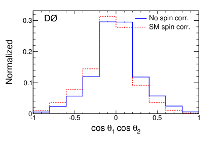
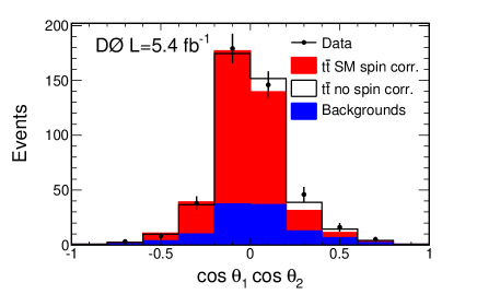
Figure 2: Left: The distribution in $\cos\theta_{1}\cos\theta_{2}$ for a sample including the NLO QCD spin correlation (C = 0.78) (red dashed line) and with no spin correlation (C = 0) (blue solid line) at the parton level, generated using MC@NLO. Right: The distribution in $\cos\theta_{1}\cos\theta_{2}$ for the entire dilepton event sample. The summed signal, including NLO QCD spin correlation (C = 0.78) (red) and all backgrounds (blue) are compared to data. The open histogram is the prediction without spin correlation (C = 0).

The right panel of Figure 2 shows the distribution observed in the data, along with the appropriately-normalized background distribution and the distributions expected for the cases of no correlation and SM correlation. On the face of it, it seems hard to distinguish the two cases. To make a quantitative statement, the most likely value of $C$ is obtained with a binned maximum-likelihood fit. Systematic uncertainties are incorporated to the fit as nuisance parameters, and the overall $t\bar{t}$ cross section is treated as a free parameter to avoid biases.

A Feldman-Cousins-based frequentist approach bib:FC is used to set confidence limits on $C$ as a function of the measured value. These are shown in Figure 3. The measured value is $C_{\mathrm{meas}}=0.10\pm 0.45$, which can be compared with the expected value of $C=0.78$. We find $-0.66<C<0.81$ at 95% confidence level. Uncertainties on the central value are shown in Table 2. Statistical uncertainties dominate by far; the leading systematic uncertainty arises from the limited Monte Carlo statistics in generating the templates. This can obviously be remedied when statistical uncertainties are reduced with more data.

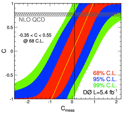
Figure 3: The 68% (inner), 95% (middle), and 99% (outer) C.L. bands of $C$ as a function of $C_{\mathrm{meas}}$ from likelihood fits to MC events for all channels combined. The yellow line indicates the most probable value of $C$ as a function of $C_{\mathrm{meas}}$, and represents the calibration of the method. The vertical dashed black line depicts the measured value $C_{\mathrm{meas}}=0.10$. The horizontal band indicates the NLO QCD prediction of $C=0.777^{+0.027}_{-0.042}$.

Table 2: Summary of uncertainties on $C_{\mathrm{meas}}$.

Source	$+$SD	$-$SD
Muon identification	0.01	$-0.01$
Electron identification and smearing	0.01	$-0.01$
PDF	0.02	$-0.01$
Top Mass	0.01	$-0.01$
Triggers	0.02	$-0.02$
Opposite charge requirement	0.00	$-0.00$
Jet energy scale	0.01	$-0.01$
Jet reconstruction and identification	0.06	$-0.06$
Normalization	0.02	$-0.02$
Monte Carlo statistics	0.02	$-0.02$
Instrumental background	0.00	$-0.00$
Background Model for Spin	0.03	$-0.04$
Luminosity	0.03	$-0.03$
Other	0.01	$-0.01$
Template statistics for template fits	0.07	$-0.07$
Total systematic uncertainty	0.11	$-0.11$
Statistical uncertainty	0.38	$-0.40$

While the measured value of $C$ agrees with the predicted value within two standard deviations, it is also consistent with no spin correlation at all. A more powerful technique is required to observe the effect with the data sample in hand.

VI Analysis II: Matrix-element-based

The second measurement makes use of the leading-order matrix element for $t\bar{t}$ production and decay, using the full event kinematics to determine the fraction of $t\bar{t}$ events in the sample that the spin correlation that is expected in the SM bib:meas2 . Matrix elements have never been used in spin-correlation measurements before, and their implementation leads to a significant improvement in sensitivity.

On an event by event basis, we can characterize whether the kinematics are consistent with the SM or with no correlation at all. This is done by calculating a probability for consistency of the event with spin correlation or non-correlation. The probability is given by

$$P_{\rm sgn}(x;H) =\frac{1}{\sigma_{\rm obs}}\int~{}f_{\rm PDF}(q_{1})~{}f_{\rm PDF}(q_{2}){\rm d}q_{1}{\rm d}q_{2}$$ (4)

$$\cdot \frac{(2\pi)^{4}\left|{\cal M}(y,H)\right|^{2}}{q_{1}q_{2}s}~{}W(x,y)~{}{\rm d}\Phi_{6}.$$

Here, $\sigma_{\rm obs}$ denotes the leading order cross section including selection efficiency, $q_{1}$ and $q_{2}$ the energy fraction of the incoming quarks from the proton and antiproton, respectively, $f_{\rm PDF}$ the parton distribution function, $s$ the center-of-mass energy squared of the $p\bar{p}$ system and ${\rm d}\Phi_{6}$ the infinitesimal volume element of the 6-body phase space. The detector resolution is taken into account through a transfer function $W(x,y)$ that describes the probability of a partonic final state $y$ to be measured as $x=(\tilde{p}_{1},\dots,\tilde{p}_{n})$, where $\tilde{p}_{i}$ denotes the measured four-momenta of the final state particles. $H$ represents the correlation hypothesis – $H=c$ corresponds to SM correlation and $H=u$ corresponds to no correlation. The appropriate matrix element is used for each case. In contrast to the template measurement, the full event kinematics plus theoretical models of $t\bar{t}$ production and decay are used, not just the lepton angles, and by adding this information, the sensitivity of the measurement is increased.

For each event, we compute

$$R=\frac{P_{\rm sgn}(H=c)}{P_{\rm sgn}(H=u)+P_{\rm sgn}(H=c)}\,,$$ (5)

Events more consistent with having SM spin correlation will tend to have $R$ close to one, while those less consistent will have $R$ closer to zero. A value of $R\simeq 0.5$ implies that it is is difficult to tell which hypothesis is more likely. The left panel of Figure 4 shows the expected distribution of $R$ for MC@NLO $t\bar{t}$ events generated with and without spin correlation. In fact, $R\simeq 0.5$ is quite common; the correlation is still a small effect. But there is some separation between the two distributions.

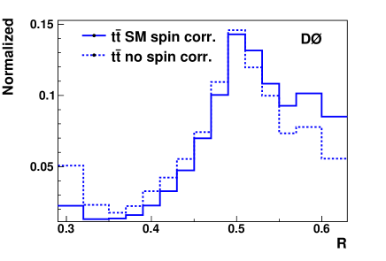
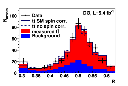
Figure 4: Left: Comparison of the discriminant $R$ between SM spin correlation $H=c$ and no spin correlation $H=u$ at parton level. The first and last bin include also the contributions from $R<0.29$ and $R>0.63$. Right: The predicted discriminant distribution $R$ for the combined dilepton event sample for the fitted $\sigma_{t\bar{t}}$ and $f_{\mathrm{meas}}$ compared to the data. The prediction with spin correlation ($f=1$) and without spin correlation ($f=0$) is shown including background.

The right panel of Figure 4 shows the distribution in $R$ observed in the data, along with the distribution expected for the background events and those for $t\bar{t}$ with and without spin correlation. By eye, one can see that the data are more consistent with the hypothesis of correlation.

The fraction of events that are consistent with SM spin correlation, $f$, is obtained from a binned likelihood fit that is very similar to that of Analysis I. This fraction is of course expected to be 100%. The confidence bands are shown in Figure 5. We find $f=0.74^{+0.40}_{-0.41}$, which is consistent with the SM. A value of $f=0$ is excluded at the 97.7% confidence level. (From ensemble testing, the measurement was expected to exclude $f=0$ at the 99.6% confidence level; if the correlation exists as expected in the SM, this measurement was “unlucky” in finding a value less than 100%.) The uncertainties on the measured value of $f$ are listed in Table 3; once again, statistical uncertainties greatly dominate.

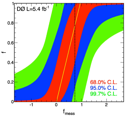
Figure 5: The 68.0% (inner), 95.0% (central), and 99.7% (outer) C.L. bands of $f$ as a function of $f_{\mathrm{meas}}$ from likelihood fits to MC events. The thin yellow line indicates the most probable value of $f$ as a function of $f_{\mathrm{meas}}$, and therefore represents the calibration of the method. The vertical dashed black line indicates the measured value $f_{\mathrm{meas}}=0.74$.

Table 3: Summary of uncertainties on $f_{\mathrm{meas}}$.

Source	$+$SD	$-$SD
Muon identification	0.01	-0.01
Electron identification and smearing	0.02	-0.02
PDF	0.06	-0.05
$m_{t}$	0.04	-0.06
Triggers	0.02	-0.02
Opposite charge selection	0.01	-0.01
Jet energy scale	0.01	-0.04
Jet reconstruction and identification	0.02	-0.06
Background normalization	0.07	-0.08
MC statistics	0.03	-0.03
Instrumental background	0.01	-0.01
Integrated luminosity	0.04	-0.04
Other	0.02	-0.02
MC statistics for template fits	0.10	-0.10
Total systematic uncertainty	0.15	-0.18
Statistical uncertainty	0.33	-0.35

VII Summary

Quark spin correlation is a phenomenon that can only be seen in $t\bar{t}$ production, thanks to the short top lifetime. However, it is a subtle effect that requires large data samples and sophisticated analysis techniques to observe. Indeed, the matrix-element technology is perhaps the most powerful, and most complex, analysis tool that is currently available for Tevatron data analyses, and it was required here to have the hope of observing the effects of interest. Two analyses of $t\bar{t}$ dilepton events at D0 have been performed. One was a template-based analysis using full reconstruction of top decays, giving a result within two standard deviations of the NLO QCD prediction, but also compatible with the no-correlation hypothesis. The other one was a matrix-element-based analysis that gives a result consistent with the SM hypothesis, and powerful enough to exclude the no-correlation hypothesis for the first time ever. Both analyses are statistics limited, with only about half of the final D0 Run II data sample analyzed so far. Thus, there is great potential for improving the precision of the measurements in the near future.

- (1) W. Bernreuther, A. Brandenburg, Z.G. Si and P. Uwer, Phys. Lett. B539, 235 (2002).
- (2) Figure lifted from Greg Mahlon’s presentation at the 3rd International Workshop on Top-Quark Physics, Brussels, Belgium, June 2010. See also M. Jezabek and J.H. Kuhn, Phys. Lett. B329, 317 (1994) and Reference 1.
- (3) V.M. Abazov et al. (D0 Collaboration), Phys. Lett. B702, 16 (2011).
- (4) B. Abbott et al. (D0 Collaboration), Phys. Rev. Lett 85, 256 (2000).
- (5) G. Feldman and R. Cousins, Phys. Rev. D57, 3873 (1998).
- (6) S. Frixione and B.R. Webber, J. High Energy Phys. 0206, 29, (2002).
- (7) V.M. Abazov et al. (D0 Collaboration), Phys. Rev. Lett. 107, 032001 (2011).