E-BOSS: An Extensive stellar BOw Shock Survey. I: Methods and First Catalogue

Abstract

Context. Bow shocks are produced by many astrophysical objects where shock waves are present. Stellar bow shocks, generated by runaway stars, have been previously detected in small numbers and well-studied. Along with progress in model development and improvements in observing instruments, our knowledge of the emission produced by these objects and its origin can now be more clearly understood.

Aims. We produce a stellar bow-shock catalogue by applying uniform search criteria and a systematic search process. This catalogue is a starting point for statistical studies, to help us address fundamental questions such as, for instance, the conditions under wich a stellar bow shock is detectable.

Methods. By using the newest infrared data releases, we carried out a search for bow shocks produced by early-type runaway stars. We first explored whether a set of known IRAS bow shock candidates are visible in the most recently available IR data, which has much higher resolution and sensitivity. We then carried out a selection of runaway stars from the latest, large runaway catalogue available. In this first release, we focused on OB stars and searched for bow-shaped features in the vicinity of these stars.

Results. We provide a bow-shock candidate survey that gathers a total of 28 members which we call the Extensive stellar BOw Shock Survey (E-BOSS). We derive the main bow-shock parameters, and present some preliminary statistical results on the detected objects.

Conclusions. Our analysis of the initial sample and the newly detected objects yields a bow-shock detectability around OB stars of $\sim$ 10 per cent. The detections do not seem to depend particularly on either stellar mass, age or position. The extension of the E-BOSS sample, with upcoming IR data, and by considering, for example, other spectral types as well, will allow us to perform a more detailed study of the findings.

1 Introduction

Many astrophysical objects perturb the interstellar medium and produce different kinds of observable structures. Early-type stars with large peculiar velocities (termed runaway stars) are one example of the perturbing agent. They are responsible for the generation of stellar bow shocks.

Runaway stars have been studied for several decades. There are currently two proposed mechanisms for the origin of their high velocities (Hoogerwerf et al. 2000). One is the binary supernova scenario (BSS, Zwicky 1957, Blauuw 1961) and the other is the dynamical ejection scenario (DES, Poveda et al. 1967, Gies & Bolton 1986). In the BSS, the runaway star that was originally part of a binary system, acquires a high speed when its companion explodes as a supernova. In the context of the DES, the runaway star achieves its velocity thanks to the dynamical interaction with one or more stars. In some cases, the trajectory of the stars and the original systems can be reconstructed, and the mechanism that has kicked the star can be identified. The gathered evidence has not always enabled strong conclusions to be made (see for instance the dissenting findings by Comerón & Pasquali 2007 and Gvaramadze & Bomans 2008). Studies such as Moffat et al. (1998) of runaway stars suggest that the BSS is slightly more likely, and that those stars with significant peculiar supersonic motion relative to the ambient ISM, tend to form bow shocks in the direction of the motion.

Abundant studies of individual or smaller groups of runaway stars can be found. However, compilations of large number of high velocity stars are scarce. A good example is the Galactic O-Star Catalog (GOSC, Maíz Apellániz et al. 2004), which contains the physical properties of about 40 of these stars. Tetzlaff et al. (2010) carried out an extensive kinematical and probability study, that allowed us to identify thousands of runaway stars. The authors used the Hipparcos catalogue (Perryman et al. 1997) and built a database of $\sim$ 2500 objects.

The effects of runaway stars on the environment and the interaction between those stars and the interstellar medium (ISM) have been widely documented. A fundamental contribution can be found in Van Buren and McCray (1988), who presented a list of 15 bow shock-like candidates, found while studying Galactic HII regions detected in IRAS (Infrared Astronomical Satellite) data. Their study triggered an extended search for stellar bow-shock candidates, which resulted in almost 60 similar sources of which around 20 were actually candidates (Van Buren et al. 1995, Noriega-Crespo et al. 1997: NC97). Some of the candidates were studied by Brown & Bomans (2005), using the H${\alpha}$ all-sky survey (SHASSA/VTSS). They searched images of 37 objects of the list of Van Buren et al. (1995) and detected 8 bow shocks. They also calculated environmental parameters and in all the cases they found consistency with the features of the warm ionized medium.

In the past few years, searches of relatively small sky regions have revealed more stellar bow shocks. Povich et al. (2008) reported the discovery of six stellar bow shocks in the star-forming regions M 17 and RCW 49 from Spitzer GLIMPSE (Galactic Legacy Infrared Mid-Plane Survey Extraordinaire) images. By combining 2MASS (Two Micron All-Sky Survey), Spitzer, MSX (Midcourse Space eXperiment), and IRAS data, they obtained the SEDs of the bow shocks and stars associated with them. Other 10 bow-shock candidates were found by Kobulnicky et al. (2010) using mid-IR images from the Spitzer Space Telescope Cygnus X Legacy Survey. Arnal et al. (2011) exposed a study of the surrounding emission related to the star HD 192281, a member of the OB association Cygnus OB8. They analyzed neutral hydrogen, radio continuum, molecular gas (CO) emission and infrared (IR) data, and derived several parameters of the medium. They concluded that HD 192281 seems to generate a stellar bow shock and it is possible that triggered star formation is underway. Bow shocks have been seen around some massive X-ray binaries, such as Vela X-1 (Kaper et al. 1997) and 4U 1907+09 (Gvaramadze et al. 2011a).

Gvaramadze et al. (2011b) carried out a search for OB stars running away from the young stellar cluster NGC 6357. They discovered seven bow shocks, and thoroughly discussed the scenario for these structures to develop.

During the investigation of the outskirts of Cygnus OB2, Comerón & Pasquali (2008) discovered a bow-shaped structure close to the high mass runaway star BD +43° 3654. From spectroscopic data, they re-classified the star and derived its stellar mass, ranking the star as one of the three most massive runaways known in the Milky Way. Stellar proper motions as well as MSX observations confirmed that the bow shock could be produced by the star, in turn probably a former member of the mentioned association. In a subsequent publication, Benaglia et al. (2010) carried out a study of the bow shock produced by BD +43° 3654, and evaluated whether the structure could give rise to high energy emission. By means of dedicated VLA observations, they calculated the spectral index in the region of the bow shock and measured values compatible with a non-thermal radiation origin. Assuming that there is a population of relativistic particles, they estimated the SEDs generated by different radiative processes.

In spite of these studies, numerous questions remain to be answered. How common are stellar bow shocks? In which conditions are they produced and detected? Questions such as how the spectral type, velocity, stellar wind, coordinates of the star, and other parameters influence the formation of a bow shock will be more clearly addressed as more examples are analyzed.

In this paper, we introduce the Extensive BOw Shock Survey (E-BOSS) generated by means of on-line available data from different missions. We used the first-release Wide-field Infrared Survey Explorer (WISE) images, as a tool to detect new structures and to contribute to what is known about those already studied.

In the next section, we briefly discuss the theoretical background and analyze the conditions that could increase the probability of detecting a stellar bow shock. Section 3 describes the procedure followed to obtain the sample in which we search for bow-shock candidates. In Section 4, we present the bow shocks found and characterize them. Section 5 shows the statistics performed, and Sect. 6 has a corresponding discussion. In the last section, we comment on the immediate prospects.

2 Theoretical considerations

Runaway stars move through the interstellar medium (ISM) with velocities that overcome the field stars velocities and the sound of speed in the ISM. They shock the ISM and produce the so-called bow shocks that sweep up the ISM matter into thin, dense shells (Wilkin 1996). The theoretical study of bow shocks has been developed not only from an analytical point of view but also with numerical simulations.

Wilkin (1996) derived analytical exact solutions for stellar wind bow shocks in the thin-shell limit, stressing the importance of the conserved momentum within the shell. He developed a simple method to reproduce the shape of the shell, mass column, and velocity of the shocked gas throughout the shell. Later, Wilkin (2000) improved the model studying the modifications of the bow shocks in two cases where: (i) a star moves supersonically with respect to an ambient medium with a density gradient perpendicular to the stellar velocity, and (ii) a star with a mis-aligned, axisymmetric wind moves in a uniform medium. He found that the region of the stand-off point (where ambient and wind pressures balance each other) is tilted in both cases. In that way, the star does not lie in the line that divides the bow shock into two halves.

Dgani et al. (1996a, 1996b) peformed a stability analysis of thin isothermal bow shocks. In the first paper, they showed that the bow shocks produced by stars with fast stellar winds are more stable than those generated by slow winds. In the second article, the authors then investigated non-linear instabilities and run numerical simulations to solve the problem. They proposed that the slower the wind, the highest the instability. They also applied the model to the star $\alpha$ Cam and concluded that the clumps observed might be explained by the instabilities.

Comerón & Kaper (1998) conducted a semi-analytical study of bow shocks produced by OB runaway stars and derived expressions that suggest different results from those obtained with the assumption of instantaneous cooling of the shocked gas (Wilkin 1996). They ran numerical simulations that reveal a wealth of details in the formation, structure, and evolution of the bow shocks. These features strongly depend on the conditions of the medium and star. The bow shocks can either form or not; and if they do form, they can be either stable, unstable, or layered.

To complete the study of bow shocks and improve the models, they need to be observed and analyzed. In principle, owing to the presence of the shocks that the runaway stars produce in the ISM, the dust is heated and in that way re-radiates at infrared wavelengths. As we describe in other sections, bow shocks have been observed at infrared (e.g. van Buren et al. 1995, NC97), optical (e.g. Brown & Bomans 2005), and -in a few cases- radio wavelengths, and will eventually be detected at high energy waves (Benaglia et al. 2010).

3 The making of the E-BOSS sample

We searched for stellar bow shocks in various different databases described later. We account for a number of criteria that help us to identify new stellar bow shocks.

1. We examined the surroundings of early-type runaway stars, as these have high velocities and strong winds that sweep up interstellar matter and also high luminosities that contribute to the dust heating.

2. We selected nearby stars ($d<$ 3 kpc), which thus have brighter bow shocks.

We generated the initial sample in two different ways. We considered first bow shock candidates that had previously been detected in the IRAS data (NC97). Secondly, we carried out a systematic search around runaway stars that could produce bow shocks, using the catalogue of Tetzlaff et al. (2010). The next section describes the process in more detail. In the rest of the paper, we divide the E-BOSS sample into two groups, groups 1 and 2.

3.1 Group 1

For this group, we took the bow shock candidates database of NC97. These authors searched for bow shocks and other features at IR wavelengths from the HiReS-IRAS maps. Table 1 lists the 56 objects that are OB stars from NC97, hereafter called group 1 (the WR stars HD 50896 and HD 192163, from the original list, were excluded).

3.2 Group 2

The second group was extracted from the catalogue of Tetzlaff et al. (2010). From a sample of 7663 young stars observed by Hipparcos (Perryman et al. 1997), the authors built a catalogue of 2546 runaway stars candidates. Their study lists stellar names, velocities, spectral types, ages, and masses. From this last list, we found 244 stars of spectral type O to B2. We list this 244 stars in Table 2; they comprise what we call hereafter group 2. A total of 17 stars are common to both groups.

3.3 Information collation

We used the NASA/IPAC Infrared Science Archive to gather relevant infrared and sub-millimeter missions data (IRAS, MSX, WISE, Spitzer, etc). In practice, data from MSX and WISE have proven to be the most useful. In particular, WISE has discovered various bow shocks. Although the published WISE data covers half of the sky, in effect, it covers more than two thirds of both group 1 and group 2 samples. When further data becomes available, it will be added to a subsequent release of the E-BOSS sample.

In addition to the infrared data, we searched for bow shock emission at H$\alpha$, using the Virginia Tech. Spectral Survey (VTSS, Dennison et al. 1997) and the Southern Hemispheric H$\alpha$ Sky Survey Atlas (SHASSA, Gaustad et al. 2001). These surveys cover most of the sky with a spatial resolution of 0.8′ for SHASSA and 1.6′ for VTSS. We did not find any convincing bow shock candidates for either our group 1 or group 2 sample. This is in contrast to Brown & Bomans (2005), who found 8 possible bow shock candidates, starting with a target list of 37 stars from van Buren et al. (1995). We note that the stars are often located in complex H$\alpha$ emission regions making identification of a bow shock feature difficult. In some cases, we did detect possible H$\alpha$ emission from a bow shock but which is not coincident with a clear bow shock detected by WISE (for example, HD 48099 and HD 149757). In these cases, we relied on the infrared detection.

The detection of radio emission and the measurement of a non-thermal radio spectral index coincident with the location of the bow-shock candidate related to the star BD $+$43° 3654 encouraged us to check for low frequency radio emission around the E-BOSS members. We used the postage stamp server for NRAO/VLA Sky Survey (NVSS, Condon et al. 1998), which returns radio images of the sky in various formats. Most of the radio maps contain only point sources, which are not particularly related to the IR features. However, three E-BOSS objects, apart from BD +43° 3654, correspond interesting comma-shaped radio sources at 1.4 GHz. A thorough investigation based on dedicated radio observations towards these candidates, HIP 88652, HIP 38430, and HIP 11891 is under way (Peri et al., in preparation).

4 Results

4.1 Group 1

We searched for WISE and MSX data toward the 56 group-1 targets, at all available wavelengths, with a field size of 1 sq degree. About 55% of the targets have MSX data, and 70% have WISE data. Table 1 gives the Hipparcos number, alternative names, and the spectral type of the stars as in NC97, or updated from GOSC (Maíz Apellániz et al. 2004) whenever possible. Columns 4 and 5 list the results obtained with MSX and WISE. We identified several types of structures around the stars that are represented with different symbols in Table 1. The categories are: a point source at the position of the star, diffuse emission in the vicinity of the star, no emission, a bow-shaped emission feature, a bubble candidate, and extended emission in the field. A ’?’ symbol implies doubtful feature. The last column reproduces the results of NC97. Two special cases are noted in the table. Cappa et al. (2008) studied the environs of HD 92206, and identified an extended HII region. The star HD 36862 is very close to HD 36861 (O8III); they both belong to the rich cluster $\lambda$ Ori (Bouy et al. 2009), are not single isolated objects, and have a large spatial velocity. In both cases, a bow shock might be hidden and we discarded these two objects from our sample.

We found 18 bow-shock candidates (BS-C) out of the 56 stars of group 1 (Table 1). Of the 18 BS-C, 3 of them were detected with MSX (one is the case of BD +43^∘ 3654) and the other 15 with WISE. Out of a total of 18 BS-C, 14 were also classified as BS-C by NC97 (see Table 1). A total of 4 new BS-C were found here, related to HIP 24575, HIP 38430, HIP 77391, and HIP 114990. We believe that the different results between Group 1 stars and NC97 are due to the high resolution and sensitivity of the more recent data.

4.2 Group 2

We list the 244 O-B2 runaway candidates extracted from Tetzlaff et al. (2010) in Table 2. We searched the WISE data to identify BS-C. The table is divided into two parts: the upper part contains those stars for which WISE data were released, and the lower portion where they were not.

We found a total of 17 BS-C, marked with bold font in the top part of Table 2; seven of them had been identified in group 1.

4.3 The E-BOSS sample

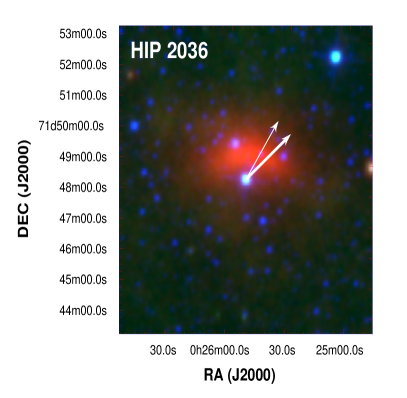
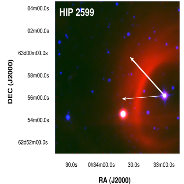
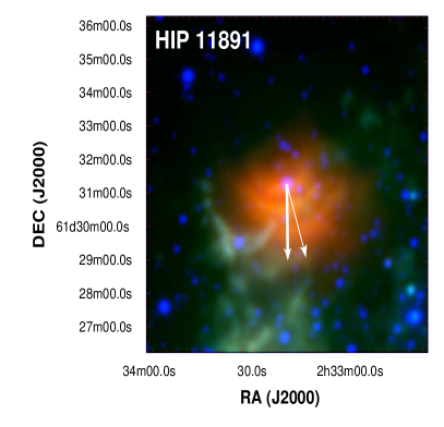
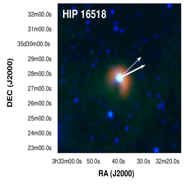
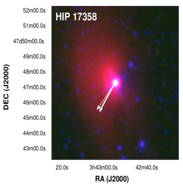
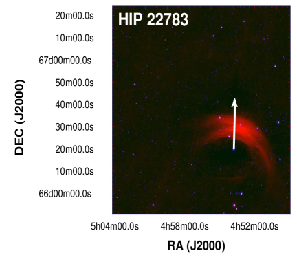
Figure 1: WISE images of the bow shock candidates around 6 OB stars. Color mapping: blue=3.4 microns; green=12.1 microns; red=22.2 microns. The color scales are in data numbers (DNs); the WISE data is not calibrated in their surface brightness. The vectors indicate the direction of the star proper motion: the thicker one represents the one derived from Hipparcos data by van Leeuwen 2007; the thinner one is the same but corrected for the ISM motion caused by Galactic rotation. The vectors length are not scaled with the original values.

The 28 objects of the E-BOSS sample are shown in Figures 1 to 5. In Table 3, the star name is given in the first column, the group membership in column 2, and Galactic coordinates in columns 3 and 4. Spectral types are in column 5. The distances, in column 6, were taken from several sources, namely Megier et al. (2009), Mason et al. (1998), Schilbach & Röser (2008), Hanson (2003), and Thorburn et al. (2003), or derived from Hipparcos parallaxes (van Leeuwen 2007). The wind terminal velocities $v_{\infty}$ are either from Howarth et al. (1997) or derived using table 3 of Prinja et al. (1990). To compute the stellar mass-loss rates $\dot{M}$, we used the routine described by Vink et al. (2001), and stellar parameters derived from standard models (e.g. Martins et al. 2005). The stellar tangential velocities $v_{\rm tg}$ were taken from Tetzlaff et al. (2010), or derived from proper motions (van Leeuwen 2007, see last two columns of Table 3). Radial velocities $v_{\rm r}$ are from the Second Catalogue of Radial Velocities with Astrometric Data (Kharchenko et al. 2007).

In Figs. 1 to 5, we show the WISE and MSX images of the 28 BS-C. Superimposed on the images, we have plotted with arrows two directions, representing the proper motion of the star derived by van Leeuwen (2007), and that of the corrected proper motion after taking into account the Galactic rotation of the ISM at the location of the star (as done for example in Comerón & Pasquali 2007 and Moffat et al. 1998, 1999).

For each BS-C, we measured geometrical parameters, such as the spatial extent $l$, the width $w$, and the distance from the star to the midpoint of the bow shock structure $R$ (Table 4, columns 2 to 7).

The ISM ambient density in the vicinity of the star $n_{\rm ISM}$ can be estimated using the expression that gives the so-called stagnation radius $R_{0}$ (see Wilkin 1996 for definition and details)

$$R_{0}=\sqrt{\frac{\dot{M}v_{\infty}}{4\pi\rho_{\rm a}v_{*}^{2}}}\,,$$

where the ambient medium density is $\rho_{\rm a}=\mu\,n_{\rm ISM}$ and $v_{*}$ is the spatial stellar velocity. We estimated the volume density of the ISM in H atoms at the bow shock position assuming $R_{0}\sim R$, a mass per H atom $\mu=2.3\times 10^{-24}$ g, and the helium fractional abundance $Y=0.1$. The values obtained for $n_{\rm ISM}$ are given in column 8 of Table 4, and should be interpreted with caution. In many cases, the width of the bow shock is substantial compared to $R$, which adds an uncertainty to the $R_{0}$ values used in the last equation.

There are additional factors that might affect the values of $R_{0}$ and $n_{\rm ISM}$, such as errors in the mass-loss rate due to clumping, in addition to the potential source of errors in the parameters used, as described above.

5 Statistics

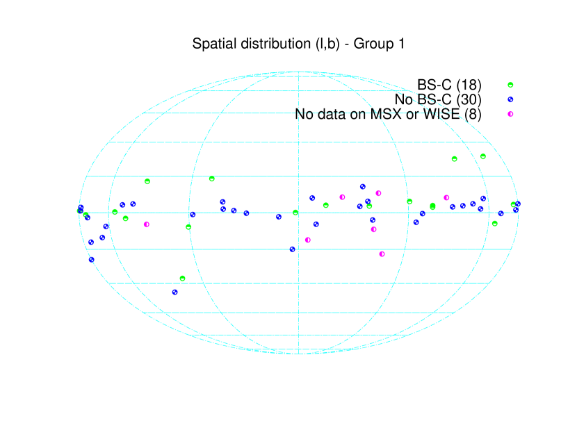
Figure 6: Distribution on the (l,b) plane of group-1 stars.

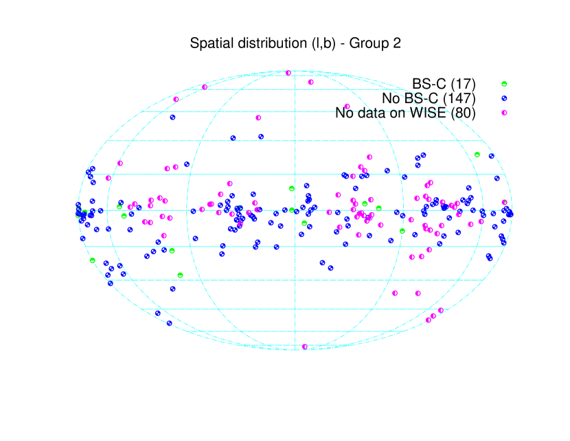
Figure 7: Distribution on the (l,b) plane of group-2 stars.

In Figs. 6-7, we present the $(l,b)$ distribution of group 1 and group 2 stars, showing those with and without bow shocks. There does not seem to be any preferential location for stars with bow shocks. We note that there are no bow shocks at high latitudes, but that the small number of stars there means we cannot say anything conclusive.

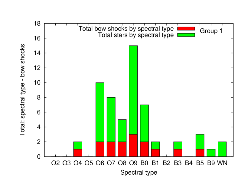
Figure 8: Distribution of group-1 stars by spectral types.

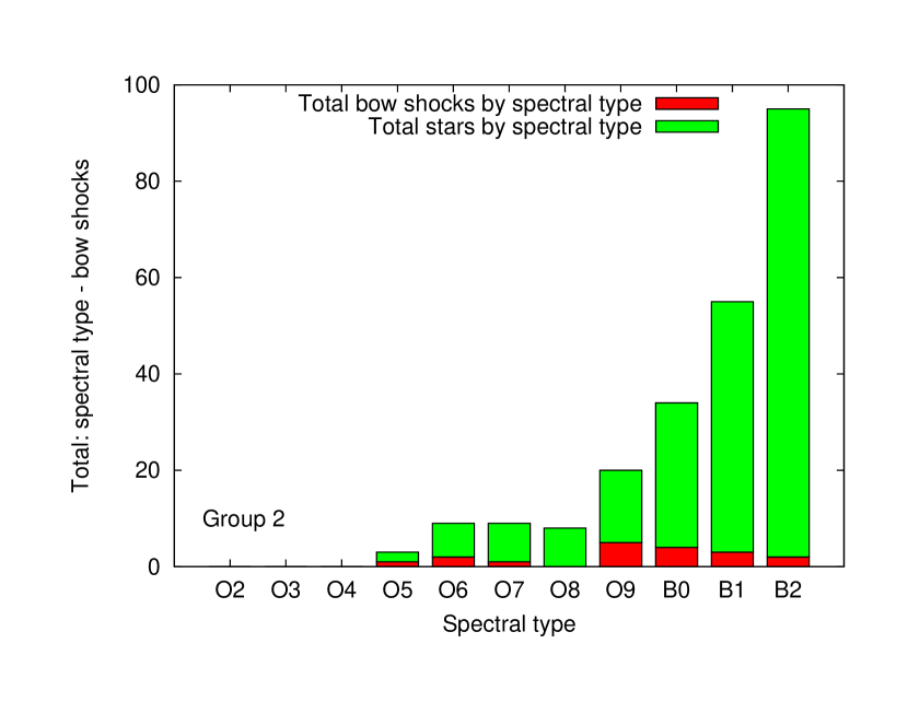
Figure 9: Distribution of group-2 stars by spectral types.

Figs. 8-9 show the occurrence of bow shocks as a function of spectral type for each group. We might have expected more detections of bow shocks from the more massive, earlier-type, or fastest stars, which is not seen. The number of stars in each subtype grows with later spectral types, probably reflecting that there is no strong bias in the Group 2 stellar sample.

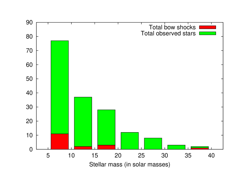
Figure 10: Distribution of group-2 stars by stellar mass (5 M_⊙ binning).

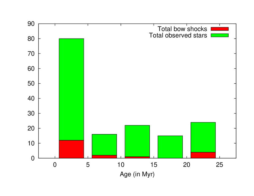
Figure 11: Distribution of group-2 stars by age (5 Myr binning).

Figs. 10-11 show that bow shocks were detected around both the lower mass stars and the youngest stars, but the very small numbers in many of the bins prevents us to draw any clear conclusion.

6 Discussion

The E-BOSS sample introduced here constitutes the most substantial sample of stellar bow shocks and should provide a reliable basis to more detailed studies of the structure and formation of bow shocks.

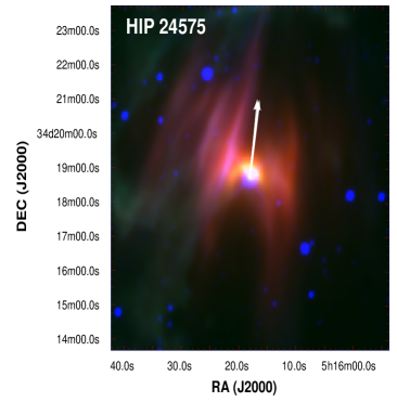
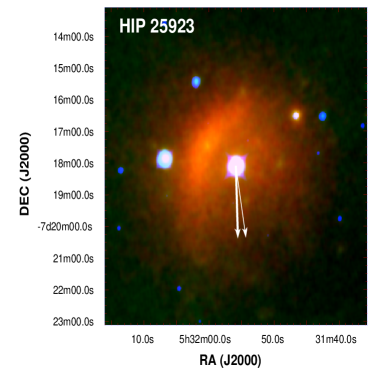
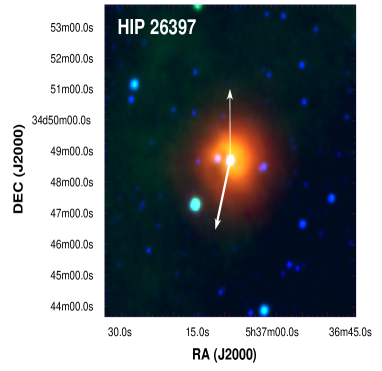
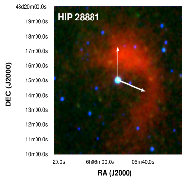
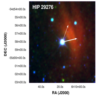
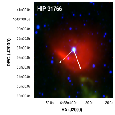
Figure 2: Same as in Figure 1, for another six OB stars.

For group 1, the availability of MSX and WISE images has enabled us to improve previous results, which relied on the IRAS data. Some structures were identified as bow shocks, others rejected, and in some cases new bow shocks were revealed. One interesting example is the feature around HD 34078 (HIP 24575). The IRAS data, discussed in NC97, revealed an excess of emission at 60$\mu$m, but no discernible bow shock. With the WISE bands, two structures can be clearly seen (Fig. 2). There are filaments around the star mainly at longer wavelengths (red=22.2 microns), and a typical bow-shaped feature becomes visible in the longer bands (red=22.2 microns and green=12.1 microns) in the direction of the stellar motion. Another example from group 1 is the object related to the B5 III star HD 22928 (HIP 17358). The combination of low mass-loss rate and wind terminal velocity, with a high stellar velocity leads to the formation of a bow shock very close to the star. This situation results in a very large derived value of the ISM density (Table 4). The stellar motion is dominated by the tangential velocity, and is a nearby star. These help us to more clearly resolve the bow shock.

The strategy we adopted here for group 2, beginning with the early-type runaways, which are most likely to form bow shocks, has been successful in identifying a significant number of new bow shocks. These results support the hypothesis that some runaway stars (around 10%) produce detectable bow shocks. There are many possible reasons why a detectable bow shock is not formed, such as a low-density ISM, an extremely high stellar velocity, or a low mass-loss rate, the inclination of the stellar velocity vector with respect to the plane of the sky, and confusion with strong field sources.

The current release of WISE data covers around 57 per cent of the sky, but covers a slightly larger fraction of the Galactic plane. For our group 2 sample (244 stars), around 67 per cent of the stars were covered in the first WISE data release (164 stars). A total of 17 of these were found to have bow shocks (a detection rate of $\sim$ 10 per cent). On the basis of these statistics, we would expect to find around 8 additional bow shock candidates in the remaining 80 group 2 sources.

Returning to the detected BS-C, several bow shocks in both group 1 and group 2 show a complex layered structure, such as HD 30614 (HIP 22783), HD 42933 (HIP 29276), and HD 15629 (HIP 11891). In many cases, but not all, the structures are aligned with the stellar velocity. An example of a misaligned bow shock candidate is HD 36512 (HIP 25923). We include this object in the sample because at this stage we lack any precise knowledge of the true stellar velocity.

HD 48099 (HIP 32076) is maybe the most classic example of a bow shock, and this object will be the subject of a future detailed study that will include modeling of the infrared emission in the formation of a bow shock del Valle et al., in preparation).

With this sample, we will be able to investigate the IR luminosity and dust temperature and compare the scaling of these quantities with stellar parameters (van Buren & McCray 1998), and also detectability (Stevens et al., in preparation).

The current sample is insufficiently large to distinguish properties according to stellar luminosity class, binarity status, or particular stellar classes, such as Of-type stars. However, when new data are released, the situation will improve.

7 Summary and prospects

We have discovered a significant number of bow shock candidates around early-type runaway stars providing a higher quality sample of bow shocks, the E-BOSS sample. For the set, we have determined a number of parameters of these objects. We have found no strong trends concerning the frequency of bow shocks with stellar mass, position, age, velocity, and spectral type.

In terms of future work, extending our study to later spectral types will allow us to systematically search for and investigate radiative bow shocks (see for example Gáspár et al. 2008). The extensive Tetzlaff et al. (2010) database will also serve as a starting point for that study. We will also incorporate in forthcoming E-BOSS versions other runaway databases together with individual objects from the literature.

Detailed studies of individual objects will help us to more clearly understand the stellar winds of the bow-shock producer stars, the medium in which they travel, and the stellar history, among other things. We plan to continue our studies of individual objects in the E-BOSS sample, as well as statistical studies of the global sample.

Table 1: Star members of Group 1.

HIP	HD/BD/Other	Spectral type	MSX	WISE	1997
1415	1337	O9IIInn+…	–	–
2599	2905 / $\kappa$ Cas	B1Iae	$\star$	$\supset$	$\supset$
3478	4142	B5V	–	$\star$	$\bullet$
13296	17505	O6Ve	$\star$	$\bullet$*	$\medcirc$?
14514	19374	B1.5V	–	$\star$	$\bullet$
15063	19820	O8.5III	$\star$	$\star$	$\supset$?
17358	22928	B5III	–	$\supset$	$\supset$
18370	24431	O9IV-V	$\times$	$\star$	$\bullet$
22783	30614 / $\alpha$ Cam	O9.5Iae	–	$\supset$	$\supset$
24575	34078	O9.5Ve…	–	$\supset$	$\bullet$
25947	+39 1328	O9III:	$\times$	$\star$	$\bullet$
——–	36862 / $\lambda$ Ori	B0.5V	–	[a]	$\supset$
26220	37020	B0.5V	$\odot$	$\odot$	$\bullet$
26889	37737	B0II:	$\times$	$\bullet$*	$\medcirc$?
28881	41161	O8V	–	$\supset$	$\supset$
29147	41997	O7.5V	–	$\odot$	$\bullet$
29276	42933 / $\delta$ Pic	B3III+…	–	$\supset$	$\supset$
31978	47839	O7Ve	$\star$	$\odot$
32067	48099	O6e	$\star$	$\supset$	$\supset$
33836	52533	O9V	$\star$	$\bullet$	$\bullet$
34536	54662	O7III	$\star$	$\supset$	$\supset$
35415	57061 / $\tau$ CMa	O9Ib	–	$\odot$	$\supset$
38430	64315	O6e	$\supset$	$\odot$	$\bullet$
39429	66811	O4If(n)p	–	–	$\bullet$
50253	89137	O9.5III(n)p	$\times$	–	$\bullet$
——–	92206	O6.5V	[b]	–	$\bullet$
56726	101131	O6V((f))	–	$\odot$	$\bullet$
63117	112244	O9Ibe	–	$\bullet$	$\bullet$

HIP	HD/BD	Spectral type	MSX	WISE	1997
72510	130298	O5/O6	$\star$	$\supset$	$\supset$
74778	135240	O8.5V	–	$\bullet$	$\bullet$
77391	329905	O+…	$\times$	$\supset$	$\bullet$
78401	143275 / $\delta$ Sco	B0.2IVe	–	$\supset$	$\supset$
81377	149757 / $\zeta$ Oph	O9V	–	$\supset$	$\supset$
84588	156212	O+…	$\star$	$\star$
85569$\dagger$	158186	O9.5V	$\star$	$\bullet$	$\bullet$
88333$\dagger$	164492	O6	$\bullet$	$\bullet$*	$\bullet$
90320	169582	O5e	$\times$	$\bullet$	$\bullet$
91113	171491	B5	$\star$	$\odot$	$\supset$
92865	175514	O8:Vnn	$\star$	$\supset$	$\supset$
97280	186980	O7.5III…	$\times$	$\o$	$\bullet$
97796	188001	O7.5Ia…	–	$\supset$	$\supset$
98418	227018	O6.5III	$\odot$	–	$\bullet$
98530	189957	B0III	–	–	$\bullet$
101186	195592	O9.5Ia	$\supset$	–	$\supset$
———	+43 3654 / U824	O4I	$\supset$	–	$\supset$
103371	199579	O6V((f))	$\star$	–	$\bullet$
104642	202214	B0II	–	–	$\bullet$
105186	203064	O8e	$\star$	–	$\bullet$
105268	203467 / 6 Cep	B3IVe	–	–	$\supset$
107598	207538	O9V	$\bullet$	–	$\bullet$
109556	210839 / $\lambda$ Cep	O6If(n)p	$\star$	–	$\supset$
110609	212593	B9Iab	–	–	$\bullet$
110817	213087	B0.5Ibe…	–	–	$\bullet$
111841	214680	O9V	–	–	$\supset$?
114990	+63 1964	B0II	$\star$	$\supset$	$\bullet$
117957	224151	B0.5II-III	–	$\star$	$\bullet$

Table 2: Star members of group 2.

HIP	Sp.t.	HIP	Sp.t.	HIP	Sp.t.	HIP	Sp.t.	HIP	Sp.t.	HIP	Sp.t.
278	B2IV	505	O6pe	1805	B0IV	2036	B1V	2599	B1Ia	4532	B1II
4983	B2IV-V	5391	B1V	6027	B2III	8725	O8V	9538	B1V	10463	B2IV-V
10527	B0.5III	10641	B2Ib	10849	B2V	10974	B2	11099	O8.5V	11279	B2Ia
11347	B1Ib	11394	O6	11396	B2	11473	O9.5V	11792	O9V	11891	O5
12009	B1Iab	12293	B2	13736	B0II-III	13924	O7V	14514	B1.5V	14626	B1V
14777	B2	14969	B2IV	15270	B2.5IV-V	16518	B1V	16566	O	17387	B2V
18151	B1III	18350	O9.5	18614	O7.5Iab	19218	O8	21626	B2.5V	22061	B2.5V
22461	B1II-III	23060	B2V	24072	B2III	24238	B2V	24575	O9.5V	25923	B0V
26064	B2IV-V	26397	B0.5V	26889	B0II	27204	B1IV-V	27850	B1V	27941	O6
28756	B2V	29201	B0V	29276	B0.5IV	29317	B1V	29321	B2V	29563	B2V
29678	B1V	30961	B2.5IV-V	31766	O9.5II	31787	B0IV	32067	O6	32300	B0.5IV
32602	O6	32947	B2V	33300	B2V	33754	B1Ib	34536	O6	34924	B2III
34986	B0.5III	35149	B1.5III	35951	B2V	36369	O6	36778	B2V	37169	O9.5Iab
38855	B2V	39172	B2.5V	40047	O5p	44685	B2IV	45880	B2	46760	B2V
48715	B1Ib	52670	B2.5V	54572	B2V	58748	B1II	61431	B1Ib	62322	B2V
62829	B0.5III	63049	B0IV	63117	O9Ib	63170	B0.5Ia	63256	B2V	64272	B1Ib
67663	B2V	68002	B2.5IV-V	68817	B0.5V	69892	O8.5	69996	B2.5IV	70574	B2IV
70877	B2III	71264	B2V	72438	B2.5V	72510	O7.5	72710	B2	74778	O8.5V
75095	B2Ib	75141	B1.5IV	75711	B2II/III	76013	B1	76642	B2III	78145	B0.5Ia
78582	B2V	79466	B2III	80782	B1.5Iap	80945	B1Ia	81100	O6e	81122	B0Ia
81305	O9Ia	81377	O9.5V	81696	O7V	82171	B0Iab	82378	O9.5IV	82691	O7e
82775	O8Iab…	82783	O9Ia	83003	O…	83574	B2Iab	83635	B1V	84226	B1Ib
84338	B2III	84401	O9	84687	B0V	84745	B2V	85331	O6.5III	85530	B2V
85885	B2II	87397	B2III	88004	B1Iab	88496	B2V	88584	O6	88652	O9.5Iab
88714	B2Ib	89743	O9.5V	90610	B2V	90804	B2V	90950	B0Ia/Iab	91003	O7
91049	B2II	91599	B0.5V	92133	B2.4V	93118	O7.5	93796	B1Ib	93934	B2II
94934	B2IV	95408	B2V	96130	B1.5III	96362	B2V	97246	B1Ia	97545	B1V
97679	B2.5V	117514	B2V
3013	B2	38518	B0.5Ib	39429	O8Iaf	39776	B2.5III	40341	B2V	41168	B2IV
41463	B2V	41878	B1.5Ib	42316	B1Ib	42354	B2III	43158	B0II/III	43868	B1Ib
44251	B2.5V	44368	B0.5Ib	46950	B1.5IV	47868	B0IV	48469	B1V	48527	B2V
48730	B2IV-V	48745	B2III	49608	B1III	49934	B2IV	50899	B0Iab/Ib	51624	B1Ib
52526	B0Ib	52849	O9V	52898	B2III	54179	B1Iab	54475	O9II	58587	B2IV
61958	Op	65388	B2	74368	B0	89902	B2V	94716	B1II-III	97045	B0V
97845	B0.5III	98418	O7	98661	B1Iab	99283	B0.5IV	99303	B2.5V	99435	B0.5V
99580	O5e	99953	B1V	100088	B1.5V	100142	B2V	100314	B1.5Ia	100409	B1Ib
101186	O9.5Ia	101350	B0V	102999	B0IV	103763	B2V	104316	O9	104548	B1V
104579	B1V	104814	B0.5V	105186	O8	105912	B2II	106620	B2V	106716	B2V
107864	Op	108911	B2Iab	109051	B2.5III	109082	B2V	109311	B1V	109332	B2III
109556	B1II	109562	O9Ib	109996	B1II	110025	B2III	110287	B1V	110362	B0.5IV
110386	B2IV-V	110662	B1.5IV-V	110817	B0.5Ib	111071	B0IV	112482	B1II	112698	B1V
114482	O9.5Iab	114685	O7

Table 3: List of the E-BOSS bow shock candidates and corresponding stellar parameters.

Star	Group	$l$	$b$	Spectral type	$d$	$v_{\infty}$	$\dot{M}\times 10^{6}$	$v_{\rm tg}$	$v_{\rm r}$	$\mu_{\alpha}\cos\delta$	$\mu_{\delta}$
		[°]	[°]		[pc]	[km s-1]	[$M_{\odot}$ yr-1]	[km s-1]	[km s-1]	[mas yr-1]	[mas yr-1]
HIP 2036	2	120.9137	+09.0357	O9.5III+B1V	757$\pm$161a	[1200]	0.48	15.2	$-$5	$-$1.66	1.90
HIP 2599	1,2	120.8361	+00.1351	B1 Iae	1457$\pm$300a	1105	0.12	26.2	$-$2.3	3.65	$-$2.07
HIP 11891	2	134.7692	+01.0144	O5 V((f))	( 900 )	2810	1.10	11.9	$-$48	0.03	$-$2.16
HIP 16518	2	156.3159	-16.7535	B1 V	( 650 )	[500]	0.006	47.3	25	$-$8.28	3.44
HIP 17358	1	150.2834	-05.7684	B5 III	( 150 )	[500]	$<$0.001	[35]	4	25.58	$-$43.06
HIP 22783	1	144.0656	+14.0424	O9.5 Ia	1607$\pm$275a	1590	0.25	[52]	6.1	$-$0.13	6.89
HIP 24575	2	172.0813	-02.2592	O9.5 V	548$\pm$68a	[1200]	0.1	140.0	59.1	$-$3.58	43.73
HIP 25923	2	210.4356	-20.9830	B0 V	( 900 )	[1000]	0.06	16.8	17.4	$-$0.10	$-$4.87
HIP 26397	2	174.0618	+01.5808	B0.5 V	( 350 )	[750]	0.014	11.9	$-$19	0.88	$-$3.61
HIP 28881	1	164.9727	+12.8935	O8 Vn	1500b	2070	0.03	[17]	5	$-$0.82	$-$1.49
HIP 29276	1,2	263.3029	-27.6837	B1/2 III	( 400 )	[600]	$<$0.001	9.2	30.6	$-$4.90	7.41
HIP 31766	2	210.0349	-02.1105	O9.7 Ib	1414$\pm$28a	1590	1.07	6.7	58.4	$-$0.34	$-$0.83
HIP 32067	1,2	206.2096	+00.7982	O5.5V((f))+…	2117$\pm$367a	2960	0.13	23.4	31	0.84	2.55
HIP 34536	1,2	224.1685	-00.7784	O6.5V((f))+…	1293$\pm$206a	2456	0.19	14.3	58	$-$1.96	4.40
HIP 38430	1	243.1553	+00.3630	O6Vn+…	( 900 )	[2570]	0.7	[13]	28	$-$3.04	$-$0.38
HIP 62322	2	302.4492	-05.2412	B2.5 V	( 150 )	[300]	0.006	4.5	42	$-$41.97	$-$8.89
HIP 72510	1,2	318.7681	+02.7685	O6.5III(n)(f)	( 350 )	[2545]	0.27	7.4	$-$74	$-$7.49	$-$5.15
HIP 75095	2	322.6802	+00.9060	B1Iab/Ib	( 800 )	[1065]	0.14	28.6	4	$-$8.42	$-$9.18
HIP 77391	1	330.4212	+04.5928	O9 I	( 800 )	[1990]	0.25	[19]	15	$-$4.63	$-$1.84
HIP 78401	1	350.0969	+22.4904	B0.2 IVe	224$\pm$24a	[1100]	0.14	[38]	$-$7	-10.21	-35.41
HIP 81377	1,2	006.2812	+23.5877	O9.5 Vnn	222$\pm$22a	[1500]	0.02	24.4	$-$15	15.26	24.79
HIP 82171	2	329.9790	-08.4736	B0.5 Ia	845$\pm$120a	1345	0.09	65.7	$-$53.3	$-$4.64	$-$20.28
HIP 88652	2	015.1187	+03.3349	B0 Ia	( 650 )	[1535]	0.5	8.2	30	$-$1.05	$-$1.38
HIP 92865	1	041.7070	+03.3784	O8 Vnn	( 350 )	[1755]	0.04	[2]	$-$41	$-$0.78	0.46
HIP 97796	1	056.4824	-04.3314	O7.5 Iabf	2200c	[1980]	0.50	[110]	9	$-$2.03	$-$10.30
HIP 101186	1	082.3557	+02.9571	O9.7 Ia	1486$\pm$402a	[1735]	0.23	22.3	$-$28	$-$2.37	1.37
BD+43 3654	1	082.4100	+02.3254	O4 If	1450d	[2325]	6.5	[14]	$-$66.2	$-$0.44	1.3
HIP 114990	1	112.8862	+03.0998	B0 II	1400e	[1400]	0.6	[52]	$-$125.3	$-$7.86	$-$0.71

Table 4: Observational parameters of the bow shock candidates obtained from the images of MSX and WISE.

Star	$l$	$w$	$R$	$l$	$w$	$R$	$n_{\rm ISM}$	Comments
		[arcmin]			[pc]		[cm-3]
HIP 2036	4.5	1.3	1	0.99	0.29	0.22	130	Emission-line star
HIP 2599	9	1.3	3	3.81	0.55	1.27	0.4	Emission-line star
HIP 11891	4	1	1	1.05	0.26	0.26	3	Star in cluster
HIP 16518	4	1	0.7	0.76	0.19	0.13	0.2	Variable star
HIP 17358	3	1	1	0.13	0.04	0.04	600	Variable star
HIP 22783	33	10	10	15.43	4.67	4.67	0.02	Emission-line star
HIP 24575	2	0.5	0.4	0.32	0.08	0.06	3	Double or multiple star
HIP 25923	4	1	1.5	1.05	0.26	0.39	1	Variable star
HIP 26397	3	1	1	0.31	0.10	0.10	2	Star
HIP 28881	9	1.5	3	5.54	0.92	1.85	0.3	Double or multiple star
HIP 29276	5	2	2	0.58	0.23	0.23	0.003	Eclipsing binary of beta Lyr type
HIP 31766	5	2	2	2.06	0.82	0.82	0.03	Double or multiple star
HIP 32067	13	2.5	3	8.01	1.54	1.85	0.1	Emission-line star
HIP 34536	12	3	4	4.51	1.13	1.50	0.01	HII (ionized) region
HIP 38430	2	0.5	0.5	0.52	0.13	0.13	60	Emission-line star
HIP 62322	4	1.2	1	0.17	0.05	0.04	0.02	Double or multiple star
HIP 72510	4.5	0.8	1.5	0.46	0.08	0.15	0.2	Emission-line star
HIP 75095	1.5	0.5	0.5	0.35	0.12	0.12	40	Star
HIP 77391	4	1	1	0.93	0.23	0.23	30	Star
HIP 78401	25	2	6	1.63	0.13	0.39	2	Double or multiple star
HIP 81377	22	2	5	1.42	0.13	0.32	1	Be star
HIP 82171	2	0.5	0.7	0.49	0.12	0.17	1	Star
HIP 88652	6	1	1.5	1.13	0.19	0.28	2	Star
HIP 92865	11	1	3	1.12	0.10	0.31	0.003	Eclipsing binary of beta Lyr type
HIP 97796	13	2.5	6	8.32	1.60	3.84	0.02	Spectroscopic binary
HIP 101186	19	2.5	4	8.21	1.08	1.73	0.1	Emission-line star
BD+43 3654	12	3	3.5	5.06	1.27	1.48	0.2	Star
HIP 114990	3.5	0.75	1.5	1.43	0.31	0.61	0.05	Star

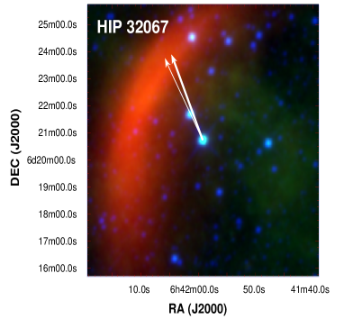
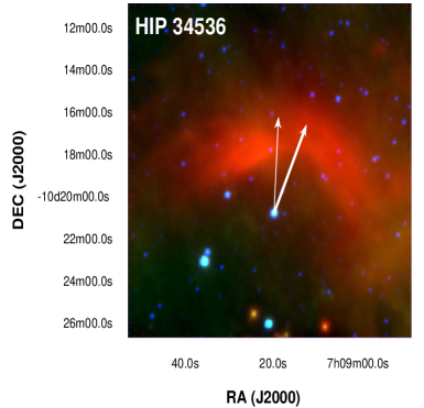
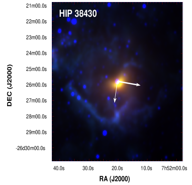
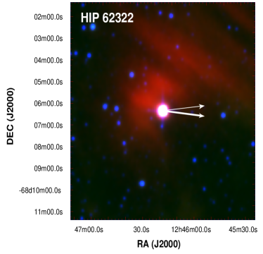
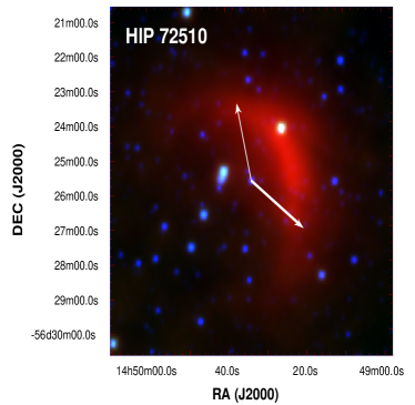
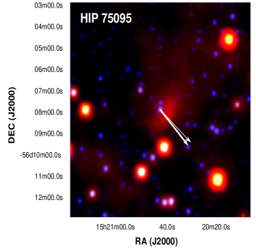
Figure 3: Same as in Figs 1-2, for another six OB stars.

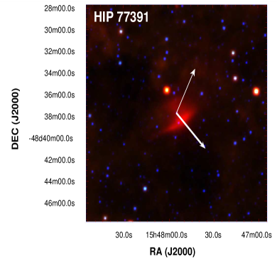
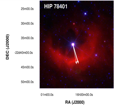
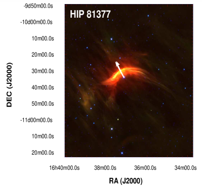
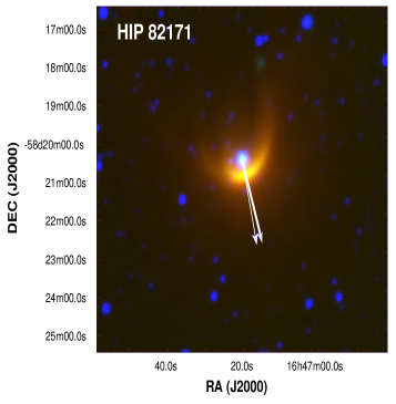
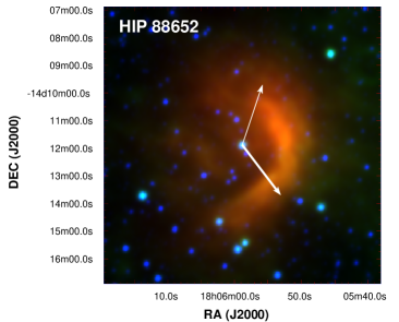
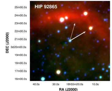
Figure 4: Same as in Figs 1-3, for another six OB stars.

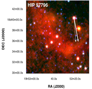
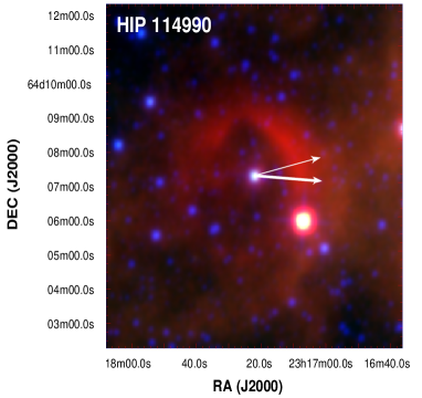
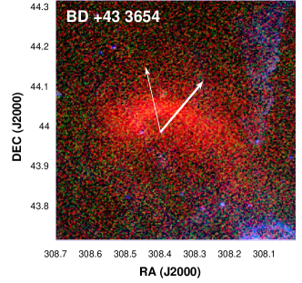
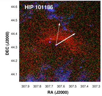
Figure 5: WISE images of bow shock candidates as in Figures 1-4, for HIP 97796 and 114990. MSX images for BD +43° 3654 and HIP 101186. Color mapping for MSX: blue=8.3 microns; green=12.1 microns; red=21.3 microns.