TWQCD Collaboration

Pseudoscalar Meson in Two Flavors QCD with the Optimal Domain-Wall Fermion

Abstract

We perform hybrid Monte Carlo (HMC) simulations of two flavors QCD with the optimal domain-wall fermion (ODWF), on the $16^{3}\times 32$ lattice (with lattice spacing $a\sim 0.1$ fm), for eight sea-quark masses corresponding to pion masses in the range 228-565 MeV. We calculate the mass and the decay constant of the pseudoscalar meson, and compare our data with the chiral perturbation theory (ChPT). We find that our data is in good agreement with the sea-quark mass dependence predicted by the next-to-leading order (NLO) ChPT, and provides a determination of the low-energy constants $\bar{l}_{3}$ and $\bar{l}_{4}$, the pion decay constant, the chiral condensate, and the average up and down quark mass.

Lattice QCD with exact chiral symmetry Kaplan:1992bt ; Neuberger:1997fp is an ideal theoretical framework to study the nonperturbative physics from the first principles of QCD. However, it is rather nontrivial to perform Monte Carlo simulation such that the chiral symmetry is preserved at a high precision and all topological sectors are sampled ergodically.

Since 2009, TWQCD collaboration has been using a GPU cluster (currently constituting of 300 Nvidia GPUs) to simulate unquenched lattice QCD with the optimal domain-wall fermion (ODWF) Chiu:2002ir ; Chiu:2009wh . Mathematically, ODWF is a theoretical framework which preserves the chiral symmetry optimally with a set of analytical weights, $\{\omega_{s},s=1,\cdots,N_{s}\}$, one for each layer in the fifth dimension Chiu:2002ir . Thus the artifacts due to the chiral symmetry breaking with finite $N_{s}$ can be reduced to the minimum, especially in the chiral regime. The 4-dimensional effective Dirac operator of massless ODWF is

$$\begin{aligned} D&=m_{0}[1+\gamma_{5}S_{opt}(H_{w})],\\ S_{opt}(H_{w})&=\frac{1-\prod_{s=1}^{N_{s}}T_{s}}{1+\prod_{s=1}^{N_{s}}T_{s}},\quad T_{s}=\frac{1-\omega_{s}H_{w}}{1+\omega_{s}H_{w}},\end{aligned}$$

which is exactly equal to the Zolotarev optimal rational approximation of the overlap Dirac operator. That is, $S_{opt}(H_{w})=H_{w}R_{Z}(H_{w})$, where $R_{Z}(H_{w})$ is the optimal rational approximation of $(H_{w}^{2})^{-1/2}$ Akhiezer:1992 ; Chiu:2002eh .

Recently we have demonstrated that it is feasible to perform a large-scale unquenched QCD simulation which not only preserves the chiral symmetry to a good precision, but also samples all topological sectors ergodically Chiu:2011dz . To recap, we perform HMC simulations of 2 flavors QCD on a $16^{3}\times 32$ lattice, with ODWF at $N_{s}=16$, and plaquette gauge action at $\beta=5.95$. Then we compute the low-lying eigenmodes of the overlap Dirac operator, and use its index to obtain the topological charge of each gauge configuration, and from which we compute the topological susceptibility for 8 sea-quark masses, each of 300 configurations. Our result of the topological susceptibility agrees with the sea-quark mass dependence predicted by the NLO ChPT Mao:2009sy , and provides the first determination of both the pion decay constant and the chiral condensate simultaneously from the topological susceptibility.

In this paper, we perform further simulations and increase the ensemble of each sea-quark mass from 300 to 500 configurations. That is, for each sea-quark mass, we generate 5000 trajectories after thermalization, and sample one configuration every 10 trajectories. Then we compute the valence quark propagators and the time-correlation function of the pseudoscalar meson operator, and from which we extract the mass $M_{\pi}$ and the decay constant $F_{\pi}$ of the pseudoscalar meson. We compare our results of $M_{\pi}$ and $F_{\pi}$ with the NLO ChPT Gasser:1984gg , and find that our results are in good agreement with the sea-quark mass dependence predicted by NLO ChPT, and from which we obtain the low-energy constants $F$, $\Sigma$, $\bar{l}_{3}$ and $\bar{l}_{4}$. With the low-energy constants, we determine the average up and down quark mass $m_{ud}^{\overline{\rm MS}}(\mathrm{2~{}GeV})$, and the chiral condensate $\Sigma^{\overline{\rm MS}}(\mathrm{2~{}GeV})$.

First, we outline our HMC simulation of 2 flavors QCD with ODWF. Starting from the ODWF action $S=\bar{\Psi}\mathcal{D}\Psi$ Chiu:2002ir on the 5D lattice, we separate the even and the odd sites (the so-called even-odd preconditioning) on the 4D lattice, and rewrite $\mathcal{D}$ as

$$\mathcal{D}(m_{q})=S_{1}^{-1}\begin{pmatrix}1&0\\ M_{5}D_{w}^{\text{OE}}&1\end{pmatrix}\begin{pmatrix}1&0\\ 0&C\end{pmatrix}\begin{pmatrix}1&M_{5}D_{w}^{\text{EO}}\\ 0&1\end{pmatrix}S_{2}^{-1},$$

where $m_{q}$ denotes the bare quark mass, $D_{w}$ denotes the standard Wilson Dirac operator plus a negative parameter $-m_{0}$ (Here $m_{0}=1.3$ in this paper.), and $D_{w}^{\text{EO/OE}}$ denotes the part of $D_{w}$ with gauge links pointing from odd/even sites to even/odd sites, and

$$\begin{aligned} M_{5}&=\left[(4-m_{0})+{\omega}^{-1/2}(1-L)(1+L)^{-1}{\omega}^{-1/2}\right]^{-1},\\ (\omega)_{ss^{\prime}}&=\omega_{s}\delta_{ss^{\prime}},\\ L=P_{+}&L_{+}+P_{-}L_{-},\quad P_{\pm}=(1\pm\gamma_{5})/2,\quad L_{-}=(L_{+})^{T},\\ (L_{+})_{ss^{\prime}}&=\left\{\begin{array}[]{ll}\delta_{s-1,s^{\prime}},&1<s\leq N_{s}\\ -(m_{q}/2m_{0})\delta_{N_{s},s^{\prime}},&s=1\end{array}\right.;\\ S_{1}&=M_{5}{\omega}^{-1/2},\quad S_{2}=(1+L)^{-1}{\omega}^{-1/2},\\ C&=1-M_{5}D_{w}^{\text{OE}}M_{5}D_{w}^{\text{EO}}.\end{aligned}$$

Since $\det\mathcal{D}=\det S_{1}^{-1}\cdot\det C\cdot\det S_{2}^{-1}$, and $S_{1}$ and $S_{2}$ do not depend on the gauge field, we can just use $C$ for the HMC simulation. After including the Pauli-Villars fields (with $m_{q}=2m_{0}$), the pseudo-fermion action for 2 flavors QCD ($m_{u}=m_{d}$) can be written as

$$S_{pf}=\phi^{\dagger}C_{PV}^{\dagger}(CC^{\dagger})^{-1}C_{PV}\phi,\quad C_{PV}\equiv C(2m_{0}).$$ (1)

In the HMC simulation Duane:1987de , we first generate random noise vector $\xi$ with Gaussian distribution, then we obtain $\phi=C_{PV}^{-1}C\xi$ using the conjugate gradient (CG). With fixed $\phi$, the system is evolved under a fictituous Hamiltonian dynamics, the so-called molecular dynamics (MD). In the MD, we use the Omelyan integrator Takaishi:2005tz , and the Sexton-Weingarten multiple-time scale method Sexton:1992nu . The most time-consuming part in the MD is to compute the vector $\eta=(CC^{\dagger})^{-1}C_{PV}\phi$ with CG, which is required for the evaluation of the fermion force in the equation of motion for the conjugate momentum of the gauge field. Here we take advantage of the remarkable floating-point capability of the Nvidia GPU, and perform the CG with mixed precision Chiu:2011rc . Moreover, the computations of the gauge force and the fermion force, and the update of the gauge field are also ported to the GPU. In other words, almost the entire HMC simulation is performed within a single GPU.

Furthermore, we introduce an auxillary heavy fermion field with mass $m_{H}$ ($m_{q}\ll m_{H}<2m_{0}$), similar to the case of the Wilson fermion Hasenbusch:2001ne . For two flavors QCD, the pseudofermion action (with $C_{H}\equiv C(m_{H})$) becomes,

$$S_{pf}^{H}=\phi^{\dagger}C_{H}^{\dagger}(CC^{\dagger})^{-1}C_{H}\phi+\phi_{H}^{\dagger}C_{PV}^{\dagger}(C_{H}C_{H}^{\dagger})^{-1}C_{PV}\phi_{H},$$

which gives exactly the same fermion determinant of (1). Nevertheless, the presence of the heavy fermion field plays a crucial role in reducing the light fermion force and its fluctuation, thus diminishes the change of the Hamiltonian in the MD trajactory, and enhances the acceptance rate. A detailed description of our HMC simulations will be presented in a forthcoming paper Chiu:HMC .

We determine the lattice spacing by heavy quark potential which is extracted from Wilson loops of size $(R_{1},R_{2},T)$, where $R_{1}$, $R_{2}$ and $T$ are the sizes in spatial and temporal directions. The spatial distance between the heavy quark and antiquark is $R=\sqrt{R_{1}^{2}+R_{2}^{2}}$. We measure all planar and non-planar Wilson loops $W$ with $a\leq R\leq 8a$ and $a\leq T\leq 8a$. Fitting the data of $W(R,T)$ to the formula $\left<W\right>=C\exp(-T\,V(R))$, we obtain the heavy quark potential $V(R)$ as a function of $R$. Here we have used all 5000 trajectories after thermalization, and we estimate the error of $V(R)$ using the jackknife method with the bin size of which the statistical error saturates. Then we fit our data of $V$ to the formula

$$V(R)=A+\frac{B}{R}+\sigma R,$$ (2)

to obtain $A$, $B$, and $\sigma$. We summarize our results in Table 1.

$m_{q}a$	$A$	$B$	$\sigma$	$\chi^{2}$/dof	$a$[fm]
0.01	0.7777(57)	-0.3814(70)	0.0577(10)	0.0329	0.1045(13)
0.02	0.7827(46)	-0.3818(41)	0.0584(9)	0.0275	0.1051(10)
0.03	0.7792(54)	-0.3789(62)	0.0595(9)	0.0368	0.1060(12)
0.04	0.7916(71)	-0.3995(78)	0.0598(13)	0.0440	0.1071(16)
0.05	0.7797(73)	-0.3798(72)	0.0615(13)	0.0456	0.1078(16)
0.06	0.7762(50)	-0.3785(44)	0.0628(11)	0.0458	0.1089(11)
0.07	0.7783(47)	-0.3855(53)	0.0633(8)	0.0255	0.1097(10)
0.08	0.7719(69)	-0.3744(64)	0.0649(12)	0.0569	0.1105(14)

Table 1: The parameters of $A$, $B$, and $\sigma$ obtained by fitting our data of heavy quark potential $V(R)$ to Eq. (2), together with the $\chi^{2}$/dof of the fit. The lattice spacing in the last column is obtained by (4).

Using the empirical formula deduced by Sommer Sommer:1993ce ,

$$F(r_{0})r_{0}^{2}=1.65,\hskip 14.22636ptF(r)\equiv\frac{d}{dr}V(r)=-\frac{B}{r^{2}}+\sigma,$$ (3)

and setting the Sommer parameter $r_{0}=0.49$ fm, we obtain the lattice spacing

$$a=r_{0}\sqrt{\frac{\sigma}{1.65+B}},$$ (4)

where the results are given in the last column of Table 1. Using the linear fit, we obtain the lattice spacing in the chiral limit, $a=0.1034(1)(2)$ fm with $\chi^{2}$/dof = 0.10, where the systematic error is estimated by varying the number of sea-quark masses. This gives the inverse lattice spacing $a^{-1}=1.908(2)(4)$ GeV.

We compute the valence quark propagator of the 4D effective Dirac operator with the point source at the origin, and with parameters exactly the same as those of the sea-quarks. First, we solve the following linear system (with even-odd preconditioned CG),

$${\cal D}(m_{q})|Y\rangle={\cal D}(2m_{0})B^{-1}|\mbox{source vector}\rangle,$$ (5)

where $B^{-1}_{x,s;x^{\prime},s^{\prime}}=\delta_{x,x^{\prime}}(P_{-}\delta_{s,s^{\prime}}+P_{+}\delta_{s+1,s^{\prime}})$ with periodic boundary conditions in the fifth dimension. Then the solution of (5) gives the valence quark propagator

$$(D_{c}+m_{q})^{-1}_{x,x^{\prime}}=\left(2m_{0}-m_{q}\right)^{-1}\left[(BY)_{x,1;x^{\prime},1}-\delta_{x,x^{\prime}}\right].$$

To measure the chiral symmetry breaking due to finite $N_{s}$, we compute the residual mass with the formula Chen:2012jy

$$\begin{aligned} m_{res}&=\left<\frac{{\rm tr}(D_{c}+m_{q})^{-1}_{0,0}}{{\rm tr}[(D_{c}^{\dagger}+m_{q})(D_{c}+m_{q})]^{-1}_{0,0}}\right>_{\{U\}}-m_{q},\end{aligned}$$ (6)

where $(D_{c}+m_{q})^{-1}$ denotes the valence quark propagator with $m_{q}$ equal to the sea-quark mass, tr denotes the trace running over the color and Dirac indices, and the subscript $\{U\}$ denotes averaging over an ensemble of gauge configurations. In Table 2, we list the residual masses for eight sea quark masses, together with those obtained by setting $\omega_{s}=1$ (polar approximation of the sign function of $H_{w}$) in the valance quark propagator. In the latter case, even though the chiral symmetry of the valence quarks is different from that of the sea quarks, it may serve as an estimate of the residual mass in the unitary limit with $\omega_{s}=1$. We see that turning on $\{\omega_{s}\}$ with $\lambda_{min}/\lambda_{max}=0.02/6.40$, the residual mass is decreased by a factor of 25-40, while the cost of computing quark propagators is increased by a factor of 2-5. Moreover, for $m_{q}a=0.01$, we also computed the residual mass with $N_{s}=32$ and $\omega_{s}=1$, and obtained $m_{res}=0.002746(13)$ which is 6 times larger than that of turning on $\{\omega_{s}\}$ with $N_{s}=16$ and $\lambda_{min}/\lambda_{max}=0.02/6.40$, while the cost is almost the same in both cases. This suggests that ODWF is a viable way to preserve the chiral symmetry on the lattice, without increasing $N_{s}$. For ODWF, using the linear fit, we obtain the residual mass in the chiral limit, $m_{res}a=0.00040(4)$, less than $5\%$ of the lightest sea quark mass. In the following, it is understood that each bare sea-quark mass $m_{q}$ is corrected by its residual mass, i.e., $m_{q}\rightarrow m_{q}+m_{res}$.

$m_{q}a$	$m_{res}$(ODWF)	$m_{res}(\omega_{s}=1)$	ratio
0.01	0.000418(31)	0.01064(17)	0.039(3)
0.02	0.000380(29)	0.01139(15)	0.033(3)
0.03	0.000269(40)	0.01047(13)	0.026(4)
0.04	0.000259(43)	0.01043(12)	0.025(4)
0.05	0.000269(41)	0.01000(13)	0.027(4)
0.06	0.000357(47)	0.01029(11)	0.035(4)
0.07	0.000248(45)	0.00988(15)	0.025(6)
0.08	0.000219(38)	0.00991(13)	0.022(4)

Table 2: The residual mass (second column) versus the sea quark mass for two flavors QCD with ODWF. The third column is the residual mass obtained by setting $\omega_{s}=1$ in the valence quark propagator. The last column is the ratio $m_{res}$(ODWF)/$m_{res}(\omega_{s}=1)$.

Using the valence quark propagator with quark mass equal to the sea-quark mass, we compute the time-correlation function of the pseudoscalar interpolator

$$C(t)=\sum_{\vec{x}}{\rm tr}\{\gamma_{5}(D_{c}+m_{q})^{-1}_{0,x}\gamma_{5}(D_{c}+m_{q})^{-1}_{x,0}\},$$

where the trace runs over the Dirac and color space. In Fig. 1, we plot $C(t)$ and its effective mass $m_{\rm eff}(t)=\cosh^{-1}\{[C(t+1)+C(t-1)]/(2C(t))\}$ for eight sea quark masses respectively. Then $\langle C(t)\rangle$ is fitted to the formula $Z[e^{-M_{\pi}t}+e^{-M_{\pi}(T-t)}]/(2M_{\pi})$ to extract the pion mass $M_{\pi}$ and the decay constant $F_{\pi}=m_{q}\sqrt{2Z}/M_{\pi}^{2}$, where the excited states have been neglected. Here we have chosen the fitting range $[t_{1},t_{2}]$ in which the effective mass attaining a plateau, and we estimate the errors of $M_{\pi}$ and $F_{\pi}$ using the jackknife method with the bin size of 15 configurations of which the statistical error saturates.

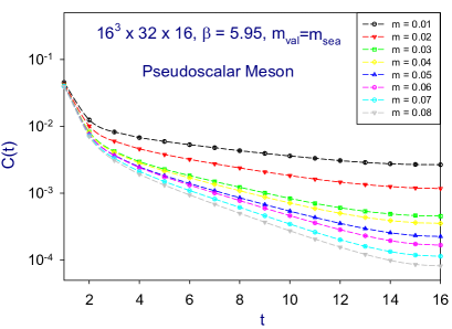
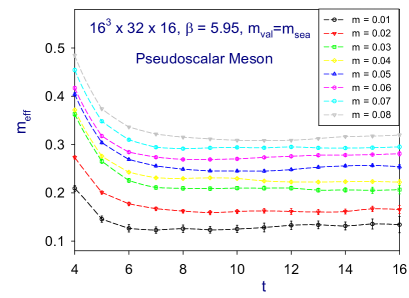
(a)	(b)

Figure 1: (color online) (a) The time-correlation function of the pseudoscalar meson for eight sea quark masses. (b) The effective mass of (a). The dashed line connecting the data points of the same sea-quark mass is for guiding the eyes.

We make the correction for the finite volume effect using the estimate within ChPT calculated up to ${\cal O}(M_{\pi}^{4}/(4\pi F_{\pi})^{4})$ Colangelo:2005gd . In Table 3, we give the values of $M_{\pi}$ and $F_{\pi}$ (with finite volume corrections), together with their finite volume correction factors computed using the formulas given in Colangelo:2005gd . In Fig. 2, we plot $M_{\pi}^{2}/m_{q}$ and $F_{\pi}$ versus $m_{q}$ respectively. For the lighest pion, $M_{\pi}L\simeq 2.0$, the formulas for finite volume correction may be unreliable, according to Ref. Colangelo:2005gd . Thus, we perform the ChPT fit with the lightest pion excluded. Then we will check whether the lightest pion falls on the curve of the ChPT fit.

$m_{q}a$	$[t_{1},t_{2}]$	$\chi^{2}$/dof	$M_{\pi}$[GeV]	$F_{\pi}$[GeV]	$1+R_{M_{\pi}}$	$1+R_{F_{\pi}}$
0.01	[8,13]	1.04	0.2275(76)	0.0970(42)	1.0815	0.7940
0.02	[9,14]	0.60	0.3089(49)	0.1060(29)	1.0301	0.9271
0.03	[6,13]	0.53	0.3672(56)	0.1114(44)	1.0158	0.9629
0.04	[6,13]	0.84	0.4135(93)	0.1170(28)	1.0091	0.9789
0.05	[7,13]	0.41	0.4586(100)	0.1217(40)	1.0055	0.9874
0.06	[7,12]	1.21	0.4976(59)	0.1240(21)	1.0037	0.9918
0.07	[9,13]	0.44	0.5327(74)	0.1263(30)	1.0026	0.9943
0.08	[6,15]	0.88	0.5654(78)	0.1270(26)	1.0020	0.9959

Table 3: Summary of the data of $M_{\pi}$ and $F_{\pi}$. The second column is the range $[t_{1},t_{2}]$ of the time-correlation function used for fitting, the third column is the $\chi^{2}$/dof of the fit, and the last two columns are finite volume corrections for $M_{\pi}$ and $F_{\pi}$ respectively.

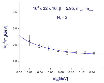
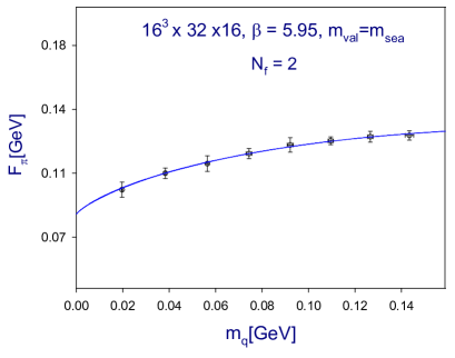
(a)	(b)

Figure 2: Physical results of 2 flavors QCD with ODWF (a) $M_{\pi}^{2}/m_{q}$, and (b) $F_{\pi}$. The solid lines are the simultaneous fits to the NLO ChPT, for seven sea-quark masses ($m_{q}a=0.02-0.08$). Note that the data points of the lightest pion are also falling on the curves of NLO ChPT fit.

Taking into account of the correlation between $M_{\pi}^{2}/m_{q}$ and $F_{\pi}$ for the same sea-quark mass, we fit our data to the formulas of NLO ChPT Gasser:1984gg

$$\frac{M_{\pi}^{2}}{m_{q}} = \frac{2\Sigma}{F^{2}}\left[1+\left(\frac{\Sigma m_{q}}{16\pi^{2}F^{4}}\right)\ln\left(\frac{2\Sigma m_{q}}{F^{2}\Lambda_{3}^{2}}\right)\right],$$ (7)

$$F_{\pi} = F\left[1-\left(\frac{\Sigma m_{q}}{8\pi^{2}F^{4}}\right)\ln\left(\frac{2\Sigma m_{q}}{F^{2}\Lambda_{4}^{2}}\right)\right],$$ (8)

where $\Lambda_{3}$ and $\Lambda_{4}$ are related to the low energy constants $\bar{l}_{3}$ and $\bar{l}_{4}$ as follows.

$$\bar{l}_{3}=\ln\left(\frac{\Lambda_{3}^{2}}{m_{\pi^{\pm}}^{2}}\right),\ \bar{l}_{4}=\ln\left(\frac{\Lambda_{4}^{2}}{m_{\pi^{\pm}}^{2}}\right),\ m_{\pi^{\pm}}=0.140\mbox{ GeV}.$$

The strategy of our data fitting is to search for the values of the parameters $\Sigma$, $F$, $\Lambda_{3}$ and $\Lambda_{4}$ such that they minimize

$$\chi^{2}=\sum_{i}V_{i}^{T}C_{i}^{-1}V_{i},\ V_{i}=\begin{pmatrix}(M_{\pi}^{2}/m_{q})_{i}-(M_{\pi}^{2}/m_{q})_{i}^{\tiny\mbox{ChPT}}\\ (F_{\pi})_{i}-(F_{\pi})_{i}^{\tiny\mbox{ChPT}}\end{pmatrix},$$

where $C_{i}$ is the $2\times 2$ covariance matrix for $M_{\pi}^{2}/m_{q}$ and $F_{\pi}$ with the same sea-quark mass.

For seven sea-quark masses corresponding to pion masses in the range $309-565$ MeV, our fit gives

$$\Sigma = [0.2140(13)(11)\mbox{ GeV}]^{3},$$ (9)

$$F = 0.0835(10)(14)\mbox{ GeV},$$ (10)

$$\bar{l}_{3} = 4.156(34)(122),$$ (11)

$$\bar{l}_{4} = 4.473(36)(46),$$ (12)

with $\chi^{2}$/dof = 0.07, where the systematic errors are estimated by varying the number of data points from 7 ($M_{\pi}\leq 565$ MeV) to 4 ($M_{\pi}\leq 459$ MeV). In Fig. (2), we see that the data points of the lightest pion also fall on the curves of NLO ChPT fit. This seems to suggest that the finite volume corrections for the lightest pion (with $M_{\pi}L\simeq 2.0$) may be correct.

To obtain the physical bare quark mass, we use the physical ratio $\left(M_{\pi}/F_{\pi}\right)^{phys}=0.135/0.093=1.45$ as the input, and solve the equation $M_{\pi}(m_{q})/F_{\pi}(m_{q})=1.45$ to obtain the physical bare quark mass $m_{q}^{phys}=0.00519(15)(18)$ GeV. From (8) and (7), we obtain the pion decay constant and the pion mass at the physical point,

$$F_{\pi} = 0.0898(12)(14)\mbox{ GeV},$$ (13)

$$M_{\pi} = 0.1298(50)(55)\mbox{ GeV}.$$ (14)

Since we have used the physical ratio 1.45 as the input, in principle, we can only regard either (13) or (14) as our predicted physical result.

In order to convert the chiral condensate $\Sigma$ and the average $m_{u}$ and $m_{d}$ to those in the $\overline{\mathrm{MS}}$ scheme, we calculate the renormalization factor $Z_{s}^{\overline{\mathrm{MS}}}(\mathrm{2~{}GeV})$ using the non-perturbative renormalization technique through the RI/MOM scheme Martinelli:1994ty , and our result is Chiu:2011np

$$Z_{s}^{\overline{\mathrm{MS}}}(\mathrm{2~{}GeV})=1.244(18)(39).$$ (15)

Then the values of $\Sigma$ and the average of $m_{u}$ and $m_{d}$ are transcribed to

$$\Sigma^{\overline{{\mathrm{MS}}}}(\mbox{2 GeV}) = [230(4)(6)\mbox{ MeV}]^{3},$$ (16)

$$m_{ud}^{\overline{{\mathrm{MS}}}}(\mbox{2 GeV}) = 4.17(13)(19)\mbox{ MeV},$$ (17)

where the systematic errors follow from those in Eqs. (9) and (15).

Since our calculation is done at a single lattice spacing the discretization error cannot be quantified reliably, but we do not expect much larger error because our lattice action is free from $O(a)$ discretization effects.

We also investigated to what extent our results of the low-energy constants depending on the chiral symmetry of the valence quark propagators. We repeated above analysis with valence quark propagators computed with $N_{s}=32$ and $\lambda_{min}/\lambda_{max}=0.01/6.4$, which has the residual mass $m_{res}a=0.000191(12)$ in the chiral limit. The low-energy constants turn out to be in good agreement with those in (9)-(12).

Moreover, our present results of the chiral condensate (16) and the pion decay constant (13) are consistent with our recent results extracted from the topological susceptibility Chiu:2011dz .

In general, our results of the $SU(2)$ low-energy constants, the chiral condensate, and the average up and down quark mass are compatible with those obtained by other lattice groups using unitary dynamical quarks with $N_{f}=2$, e.g., Ref. Noaki:2008iy . A detailed comparison with all lattice results Colangelo:2010et is beyond the scope of this paper.

To conclude, our results of the mass and the decay constant of the pseudoscalar meson are in good agreement with the sea-quark mass dependence predicted by the next-to-leading order (NLO) ChPT, and provide a determination of the low-energy constants $\bar{l}_{3}$ and $\bar{l}_{4}$, the pion decay constant, the chiral condensate, and the average up and down quark mass. Together with our recent result of the topological susceptibility Chiu:2011dz , these suggest that the nonperturbative chiral dynamics of the sea quarks are well under control in our HMC simulations. Moreover, this study also shows that it is feasible to perform large-scale simulations of unquenched lattice QCD, which not only preserve the chiral symmetry to a good precision, but also sample all topological sectors ergodically. This provides a new strategy to tackle QCD nonperturbatively from the first principles.

This work is supported in part by the National Science Council (Nos. NSC99-2112-M-002-012-MY3, NSC99-2112-M-001-014-MY3) and NTU-CQSE (No. 10R80914-4). We also thank NCHC and NTU-CC for providing facilities to perform part of our calculations.

References

- (1) D. B. Kaplan, Phys. Lett. B 288, 342 (1992); Nucl. Phys. Proc. Suppl. 30, 597 (1993).
- (2) H. Neuberger, Phys. Lett. B 417, 141 (1998); R. Narayanan and H. Neuberger, Nucl. Phys. B 443, 305 (1995).
- (3) T. W. Chiu, Phys. Rev. Lett. 90, 071601 (2003); Phys. Lett. B 552, 97 (2003); hep-lat/0303008
- (4) T.W. Chiu et al. [TWQCD Collaboration], PoS LATTICE2009, 034 (2009). [arXiv:0911.5029 [hep-lat]]
- (5) N. I. Akhiezer, ”Theory of approximation”, Reprint of 1956 English translation, Dover, New York, 1992.
- (6) T. W. Chiu, T. H. Hsieh, C. H. Huang and T. R. Huang, Phys. Rev. D 66, 114502 (2002).
- (7) T. W. Chiu, T. H. Hsieh and Y. Y. Mao, Phys. Lett. B 702, 131 (2011). [arXiv:1105.4414 [hep-lat]]
- (8) Y. Y. Mao and T. W. Chiu [TWQCD Collaboration], Phys. Rev. D 80, 034502 (2009).
- (9) J. Gasser and H. Leutwyler, Nucl. Phys. B 250, 465 (1985).
- (10) S. Duane, A. D. Kennedy, B. J. Pendleton and D. Roweth, Phys. Lett. B 195, 216 (1987).
- (11) T. Takaishi and P. de Forcrand, Phys. Rev. E 73, 036706 (2006).
- (12) J. C. Sexton and D. H. Weingarten, Nucl. Phys. B 380, 665 (1992).
- (13) T. W. Chiu et al. [ TWQCD Collaboration ], PoS LATTICE2010, 030 (2010). [arXiv:1101.0423 [hep-lat]], and references therein.
- (14) M. Hasenbusch, Phys. Lett. B 519, 177 (2001).
- (15) T. W. Chiu et al. [TWQCD Collaboration], “Monte Carlo simulation of lattice QCD with the optimal domain-wall fermion”, in preparation.
- (16) R. Sommer, Nucl. Phys. B 411, 839 (1994)
- (17) Y. C. Chen, T .W. Chiu [TWQCD Collaboration] arXiv:1205.6151 [hep-lat].
- (18) G. Colangelo, S. Durr and C. Haefeli, Nucl. Phys. B 721, 136 (2005).
- (19) G. Martinelli, C. Pittori, C. T. Sachrajda, M. Testa and A. Vladikas, Nucl. Phys. B 445, 81 (1995).
- (20) T. W. Chiu et al. [TWQCD Collaboration], “Nonperturbative renormalization of bilinear operators in lattice QCD with the optimal domain-wall fermion”, in preparation.
- (21) J. Noaki et al. [JLQCD and TWQCD Collaboration], Phys. Rev. Lett. 101, 202004 (2008)
- (22) G. Colangelo, S. Durr, A. Juttner, L. Lellouch, H. Leutwyler, V. Lubicz, S. Necco, C. T. Sachrajda et al., Eur. Phys. J. C71, 1695 (2011).