Pair excitations and parameters of state of imbalanced Fermi gases at finite temperatures

Abstract

The spectra of low-lying pair excitations for an imbalanced two-component superfluid Fermi gas are analytically derived within the path-integral formalism taking into account Gaussian fluctuations about the saddle point. The spectra are obtained for nonzero temperatures, both with and without imbalance, and for arbitrary interaction strength. On the basis of the pair excitation spectrum, we have calculated the thermodynamic parameters of state of cold fermions and the first and second sound velocities. The parameters of pair excitations show a remarkable agreement with the Monte Carlo data and with experiment.

PACS numbers: 03.75.Ss, 05.30.Fk, 03.75.Lm

1 Introduction

Recent experimental breakthroughs in the manipulation of ultracold Bose and Fermi gases have opened new prospects for advancing many-body physics ¹. The dimensionality of these gases can be controlled with optical lattices, and the interaction strength can be tuned using Feshbach resonances. The experimental control over geometry and interactions in ultracold atomic gases has turned these systems into powerful quantum simulators that can test and generalize many-body theories originally developed for solid state systems. Recently, much attention has been paid to ultracold atomic gases with strong interactions because of their possible relation to some striking natural phenomena including high-temperature superconductors and neutron stars ².

In particular, great experimental and theoretical effort has been devoted to the study of superfluidity arising from pairing in ultracold Fermi gases ³. Specifically, the effect of population imbalance (between the pairing partners) on the superfluid pairing mechanism is a topic of current investigation. Of no less interest in the context of high-temperature superconductivity is the study of the crossover between the Bardeen-Cooper-Schrieffer (BCS) and the molecular Bose-Einstein condensation (BEC) regimes.

In order to describe the superfluid phase transition as well as the broken-symmetry phase below a critical temperature $T_{c}$, several methods based on the $T$-matrix approach have been developed ^{4, 5, 6, 7, 8, 9, 10}. Amongst those, the Nozières–Schmitt-Rink (NSR) theory ⁴ and its path-integral reformulation ⁵ have been very successful and remain widely used. Here, we use an improved version of the NSR scheme, that we will denote as the Gaussian pair fluctuation theory (GPF) ^{11, 12}, and that effectively works both at low temperatures and above $T_{c}$.

As shown in Ref. ¹³, the thermodynamic properties of the superfluid Fermi gas at sufficiently low temperatures can be derived within a simple model using the spectrum of low-lying elementary excitations. In that model, the thermodynamics of the superfluid Fermi gas ¹³ is based on the fermion-boson model with phenomenological parameters whose values are determined from the Monte Carlo calculations ^{14, 16, 18, 19} (in the limit of zero temperature). The model exploited in Ref. ¹³ describes well the thermodynamic properties of a balanced unitary Fermi gas at low temperatures. Moreover it was demonstrated ²⁰ that in the BEC limit, the imbalanced Fermi superfluid indeed reduces to a simple Bose-Fermi mixture of Bose-condensed molecules and unpaired fermions. The goal of the present work is to extend these results to non-zero temperatures, and to arbitrary scattering lengths.

For this purpose, we calculate the parameters needed for the fermion-boson model from the NSR and/or GPF theories. Our results are compared with the Monte Carlo data at unitarity. We analytically derive the spectra of low-lying elementary excitations for an imbalanced Fermi gas in 3D at finite temperatures in the whole range of the BCS-BEC crossover. These spectra are obtained using the path-integral representation ⁵ of the NSR theory extended to imbalanced Fermi gases ^{21, 22} as well as the GPF approach ^{11, 12}. Using the obtained spectra of the elementary excitations, thermodynamic parameters such as the internal energy, the chemical potential, the first and second sound velocities, are calculated.

2 Formalism

2.1 Path-integral GPF approach for imbalanced Fermi gases

We consider a two-component Fermi gas within the path-integral approach. The path-integral formulation ⁵ of the NSR scheme has been extended in Refs. ^{21, 22} to the case of unequal ‘spin up’ and ‘spin down’ populations of fermions. In the present work, the treatment of the imbalanced Fermi gas is performed using the NSR scheme ^{21, 22} and its improved version, the GPF theory ¹¹ extended to the imbalanced case.

The thermodynamic parameters of the imbalanced Fermi gas are completely determined by the thermodynamic potential $\Omega$ of the grand-canonical ensemble. The thermodynamic potential $\Omega$, the same as in Refs. ^{21, 22}, is the sum of the saddle-point thermodynamic potential $\Omega_{sp}$ and the fluctuation contribution $\Omega_{fl}$. These thermodynamic potentials are provided, respectively, by the zeroth-order and quadratic terms of the expansion of the Hubbard-Stratonovich pair-field action around the saddle point.

The saddle-point thermodynamic potential for the imbalanced Fermi gas with $s$-wave pairing is ²¹

$$\Omega_{sp}=-V\int\frac{d\mathbf{k}}{\left(2\pi\right)^{3}}\left[\frac{1}{\beta}\ln\left(2\cosh\beta\zeta+2\cosh\beta E_{\mathbf{k}}\right)-\xi_{\mathbf{k}}-\frac{\Delta^{2}}{2k^{2}}\right]-V\frac{\Delta^{2}}{8\pi a_{s}}$$ (1)

where $V$ is the system volume, $\beta$ is the inverse to the thermal energy $k_{B}T$, $\Delta$ is the amplitude of the gap parameter, $a_{s}$ is the scattering length, $\xi_{\mathbf{k}}=k^{2}-\mu$ is the fermion energy, and $E_{\mathbf{k}}=\sqrt{\xi_{\mathbf{k}}^{2}+\Delta^{2}}$ is the Bogoliubov excitation energy. The chemical potentials of imbalanced fermions are expressed through the averaged chemical potential $\mu=\left(\mu_{\uparrow}+\mu_{\downarrow}\right)/2$ and the chemical potential imbalance $\zeta=\left(\mu_{\uparrow}-\mu_{\downarrow}\right)/2$. We choose the units with $\hbar=1$, the fermion mass $m=1/2$, and the Fermi energy $E_{F}\equiv\hbar^{2}\left(3\pi^{2}n\right)^{2/3}/\left(2m\right)=1$ ($n$ is the total fermion density). The fluctuation contribution to the thermodynamic potential $\Omega_{fl}$ is the same as in Refs. ^{21, 22}.

The gap parameter is found from the gap equation minimizing the saddle-point thermodynamic potential,

$$\left.\dfrac{\partial\Omega_{sp}(T,\mu,\zeta;\Delta)}{\partial\Delta}\right|_{T,\mu,\zeta}=0$$ (2)

from which we can extract $\Delta(T,\mu,\zeta)$. For an imbalanced gas, the saddle-point thermodynamic potential can have two minima: one at $\Delta=0$ and one at $\Delta\neq 0$. This can result in a first-order superfluid phase transition ²³. With our notation, we emphasize that the thermodynamic potential is a function of $T,\mu,\zeta$ (and actually $V$, but this dependency drops out). However, $\Delta$ is treated as an additional parameter on which the thermodynamic potential depends. It is this treatment of $\Delta$ as an additional parameter (in the broken-symmetry phase with $\Delta\neq 0$) that leads to a distinction between the NSR approach and the GPF approach. When calculating the gap equation one should use

$$n =-\left.\dfrac{\partial\Omega\left(T,\mu,\zeta;\Delta\right)}{\partial\mu}\right|_{T,\zeta,\Delta}-\left.\dfrac{\partial\Omega_{fl}\left(T,\mu,\zeta;\Delta\right)}{\partial\Delta}\right|_{T,\zeta,\mu}\left.\dfrac{\partial\Delta(T,\mu,\zeta)}{\partial\mu}\right|_{T,\zeta},$$ (3)

$$\delta n =-\left.\dfrac{\partial\Omega\left(T,\mu,\zeta;\Delta\right)}{\partial\zeta}\right|_{T,\mu,\Delta}-\left.\dfrac{\partial\Omega_{fl}\left(T,\mu,\zeta;\Delta\right)}{\partial\Delta}\right|_{T,\zeta,\mu}\left.\dfrac{\partial\Delta(T,\mu,\zeta)}{\partial\zeta}\right|_{T,\mu}.$$ (4)

In the standard NSR approach the last terms (involving the derivatives of $\Delta$) are omitted. The GPF approach suggested in Refs. ^{11, 12} takes into account the additional derivatives for the balanced case, and corrects the NSR densities for changes in $\Delta$ as $\mu$ and $\zeta$ are varied. The GPF method presented here is the path-integral formulation of the GPF theory of Refs. ^{11, 12} extended to the imbalanced case. As shown in Ref. ¹², the GPF theory provides the best overall agreement of its analytic results with experiment and with Monte Carlo data, except in close vicinity to $T_{c}$.

The GPF corrections are not present when one uses the saddle-point approximation and calculates

$$n_{sp} =-\left.\dfrac{\partial\Omega_{sp}\left(T,\mu,\zeta;\Delta\right)}{\partial\mu}\right|_{T,\zeta,\Delta},$$ (5)

$$\delta n_{sp} =-\left.\dfrac{\partial\Omega_{sp}\left(T,\mu,\zeta;\Delta\right)}{\partial\zeta}\right|_{T,\mu,\Delta}.$$ (6)

However, the correction terms will be relevant for the calculation of the fluctuation contributions, $n_{fl}=n-n_{sp}$ and $\delta n_{fl}=\delta n-\delta n_{sp}$. These fluctuation contributions to the density $n_{fl}$ and $\delta n_{fl}$ are given by the same expressions as in Ref. ²¹

$$n_{fl} =-\int\frac{d\mathbf{q}}{\left(2\pi\right)^{3}}\left[\frac{1}{\pi}\int_{-\infty}^{\infty}\operatorname{Im}\frac{J\left(\mathbf{q},\omega+i\gamma\right)}{e^{\beta\left(\omega+i\gamma\right)}-1}d\omega+\frac{1}{\beta}\sum_{n=-n_{0}}^{n_{0}}J\left(\mathbf{q},i\nu_{n}\right)\right],$$ (7)

$$\delta n_{fl} =-\int\frac{d\mathbf{q}}{\left(2\pi\right)^{3}}\left[\frac{1}{\pi}\int_{-\infty}^{\infty}\operatorname{Im}\frac{K\left(\mathbf{q},\omega+i\gamma\right)}{e^{\beta\left(\omega+i\gamma\right)}-1}d\omega+\frac{1}{\beta}\sum_{n=-n_{0}}^{n_{0}}K\left(\mathbf{q},i\nu_{n}\right)\right].$$ (8)

Here, $n_{0}$ is an arbitrary positive integer, and the parameter $\gamma$ lies between two bosonic Matsubara frequencies $\nu_{n_{0}}<\gamma<\nu_{n_{0}+1}$, $\nu_{n}\equiv 2\pi n/\beta$. The spectral functions $J\left(\mathbf{q},z\right)$ and $K\left(\mathbf{q},z\right)$ of complex frequency $z$ are

$$J\left(\mathbf{q},z\right) =\frac{M_{1,1}\left(\mathbf{q},-z\right)\frac{\partial M_{1,1}\left(\mathbf{q},z\right)}{\partial\mu}-M_{1,2}\left(\mathbf{q},-z\right)\frac{\partial M_{1,2}\left(\mathbf{q},z\right)}{\partial\mu}}{M_{1,1}\left(\mathbf{q},z\right)M_{1,1}\left(\mathbf{q},-z\right)-M_{1,2}^{2}\left(\mathbf{q},z\right)},$$ (9)

$$K\left(\mathbf{q},z\right) =\frac{M_{1,1}\left(\mathbf{q},-z\right)\frac{\partial M_{1,1}\left(\mathbf{q},z\right)}{\partial\zeta}-M_{1,2}\left(\mathbf{q},-z\right)\frac{\partial M_{1,2}\left(\mathbf{q},z\right)}{\partial\zeta}}{M_{1,1}\left(\mathbf{q},z\right)M_{1,1}\left(\mathbf{q},-z\right)-M_{1,2}^{2}\left(\mathbf{q},z\right)},$$ (10)

where $M_{j,k}\left(\mathbf{q},z\right)$ are the matrix elements of the pair field propagator. The matrix elements $M_{j,k}\left(\mathbf{q},z\right)$ are given by the expressions ²¹

$$M_{1,1}\left(\mathbf{q},z\right) =\int\frac{d\mathbf{k}}{\left(2\pi\right)^{3}}\left\{\frac{1}{2k^{2}}+\frac{X\left(E_{\mathbf{k}}\right)}{2E_{\mathbf{k}}}\left[\frac{\left(z-E_{\mathbf{k}}+\varepsilon_{\mathbf{k}+\mathbf{q}}\right)\left(E_{\mathbf{k}}+\varepsilon_{\mathbf{k}}\right)}{\left(z-E_{\mathbf{k}}+E_{\mathbf{k}+\mathbf{q}}\right)\left(z-E_{\mathbf{k}}-E_{\mathbf{k}+\mathbf{q}}\right)}\right.\right.$$

$$\left.\left.-\frac{\left(z+E_{\mathbf{k}}+\varepsilon_{\mathbf{k}+\mathbf{q}}\right)\left(E_{\mathbf{k}}-\varepsilon_{\mathbf{k}}\right)}{\left(z+E_{\mathbf{k}}-E_{\mathbf{k}+\mathbf{q}}\right)\left(z+E_{\mathbf{k}+\mathbf{q}}+E_{\mathbf{k}}\right)}\right]\right\}-\frac{1}{8\pi a_{s}},$$ (11)

$$M_{1,2}\left(\mathbf{q},z\right) =-\Delta^{2}\int\frac{d\mathbf{k}}{\left(2\pi\right)^{3}}\frac{X\left(E_{\mathbf{k}}\right)}{2E_{\mathbf{k}}}\left[\frac{1}{\left(z-E_{\mathbf{k}}+E_{\mathbf{k}+\mathbf{q}}\right)\left(z-E_{\mathbf{k}}-E_{\mathbf{k}+\mathbf{q}}\right)}\right.$$

$$\left.+\frac{1}{\left(z+E_{\mathbf{k}}-E_{\mathbf{k}+\mathbf{q}}\right)\left(z+E_{\mathbf{k}}+E_{\mathbf{k}+\mathbf{q}}\right)}\right].$$ (12)

Here, the distribution function $X\left(E_{\mathbf{k}}\right)$ is

$$X\left(E_{\mathbf{k}}\right)=\frac{\sinh\beta E_{\mathbf{k}}}{\cosh\beta E_{\mathbf{k}}+\cosh\beta\zeta}.$$ (13)

The derivatives in (9) and (10) within the GPF scheme are determined as mentioned above – taking into account a variation of the gap parameter. Within the NSR scheme, these derivatives are calculated assuming $\Delta$ to be an independent variational parameter.

The equation of state of the imbalanced Fermi gas is thus determined as a joint solution of the saddle-point gap equation and the number equations accounting for Gaussian fluctuations. Within both the NSR and GPF schemes, the Gaussian fluctuations do not feed back into the saddle-point gap equation.

2.2 Low-lying pair excitations

In order to obtain the spectrum of low-lying pair excitations for the imbalanced Fermi gas, we perform the long-wavelength and low-energy expansion of the matrix elements $M_{j,k}\left(\mathbf{q},z\right)$ as proposed in Ref. ¹⁰. We take into account the terms up to quadratic order in powers of $q$ and $z$, and find:

$$M_{1,1}\left(\mathbf{q},z\right) \approx A+Bq^{2}+Cz+Qz^{2},$$

$$M_{1,2}\left(\mathbf{q},z\right) \approx D+Eq^{2}+Hz^{2}.$$ (14)

The coefficients of the expansion (14) are derived straightforwardly. After some algebra, we arrive at their expression through the integrals:

$$A =\frac{1}{2\pi^{2}}\int k^{2}dk\left(\frac{1}{2k^{2}}-\frac{E_{k}^{2}+\xi_{k}^{2}}{4E_{k}^{3}}X\left(E_{\mathbf{k}}\right)-\frac{\Delta^{2}}{4}\frac{X^{\prime}\left(E_{k}\right)}{E_{k}^{2}}\right)-\frac{1}{8\pi a_{s}},$$

$$B =\frac{1}{48\pi^{2}}\int k^{2}dk\frac{2E_{k}^{4}k^{2}-3E_{k}^{4}\xi_{k}+9\xi_{k}^{3}E_{k}^{2}+14E_{k}^{2}\xi_{k}^{2}k^{2}-20\xi_{k}^{4}k^{2}}{E_{k}^{7}}X\left(E_{\mathbf{k}}\right)$$

$$+\frac{\Delta^{2}}{24\pi^{2}}\int k^{2}dk\frac{1}{E_{k}^{4}}\left(\frac{3\xi_{k}\left(E_{k}^{2}-2\xi_{k}k^{2}\right)}{E_{k}^{2}}X^{\prime}\left(E_{k}\right)\right.$$

$$\left.+\frac{6\xi_{k}^{2}k^{2}-E_{k}^{2}\left(3\xi_{k}+2k^{2}\right)}{2E_{k}}X^{\prime\prime}\left(E_{k}\right)-\frac{2k^{2}\xi_{k}^{2}}{3}X^{(3)}\left(E_{k}\right)\right),$$

$$C =-\frac{1}{8\pi^{2}}\int k^{2}dk\frac{\xi_{k}}{E_{k}^{3}}X\left(E_{\mathbf{k}}\right)-\frac{\Delta^{2}}{8\pi^{2}}\int k^{2}dk\frac{X^{\prime}\left(E_{k}\right)}{\xi_{k}E_{k}^{2}},$$

$$D =\frac{\Delta^{2}}{8\pi^{2}}\int k^{2}dk\frac{X\left(E_{\mathbf{k}}\right)}{E_{\mathbf{k}}^{3}}-\frac{\Delta^{2}}{8\pi^{2}}\int k^{2}dk\frac{X^{\prime}\left(E_{k}\right)}{E_{k}^{2}},$$

$$E =\frac{\Delta^{2}}{48\pi^{2}}\int k^{2}dk\frac{20\xi_{k}^{2}k^{2}-E_{k}^{2}\left(9\xi_{k}+6k^{2}\right)}{E_{k}^{7}}X\left(E_{\mathbf{k}}\right)$$

$$+\frac{\Delta^{2}}{24\pi^{2}}\int k^{2}dk\frac{1}{E_{k}^{4}}\left(\frac{E_{k}^{2}\left(3\xi_{k}+2k^{2}\right)-6\xi_{k}^{2}k^{2}}{2E_{k}^{2}}\left[2X^{\prime}\left(E_{k}\right)-E_{k}X^{\prime\prime}\left(E_{k}\right)\right]\right.$$

$$\left.-\frac{2k^{2}\xi_{k}^{2}}{3}X^{(3)}\left(E_{k}\right)\right),$$

$$Q =-\frac{1}{32\pi^{2}}\int k^{2}dk\frac{E_{k}^{2}+\xi_{k}^{2}}{E_{k}^{5}}X\left(E_{\mathbf{k}}\right),$$

$$H =\frac{\Delta^{2}}{32\pi^{2}}\int_{0}^{\infty}k^{2}dk\frac{X\left(E_{\mathbf{k}}\right)}{E_{k}^{5}}.$$ (15)

The low-lying pair excitations correspond to the poles of the spectral functions (9) and (10). Therefore the dispersion equation for the energies of the pair excitations $\omega=\omega_{q}$ is

$$M_{1,1}\left(\mathbf{q},\omega\right)M_{1,1}\left(\mathbf{q},-\omega\right)-M_{1,2}^{2}\left(\mathbf{q},\omega\right)=0.$$ (16)

This equation is solved expanding $\omega_{q}^{2}$ up to the terms of the order of $q^{4}$. We then obtain the energies $\omega_{q}$ in a form structurally similar to the collective excitations in Ref. ¹³:

$$\omega_{q}=\sqrt{c^{2}q^{2}+\lambda q^{4}},$$ (17)

where the parameters $c$ and $\lambda$ are related to the coefficient of the expansion (14) as follows,

$$c =\left(\frac{2A\left(B-E\right)}{C^{2}+2A\left(H-Q\right)}\right)^{1/2},$$ (18)

$$\lambda =\frac{C^{2}\left(B-E\right)\left(4A\left(BH-EQ\right)+C^{2}\left(B+E\right)\right)}{\left(C^{2}+2A\left(H-Q\right)\right)^{3}}.$$ (19)

For small pair momentum $q$, the energy of the pair excitation becomes linear in the momentum. Thus $\omega_{q}$ at small $q$ represents a Bogoliubov–Anderson mode, which is gapless in accordance with the Nambu–Goldstone theorem. The parameter $c$ has the dimensionality of velocity. In the zero-temperature limit for a balanced gas, all fermions are in the superfluid state, and the velocity parameter for the pair excitations tends to the first sound velocity for the whole fermion system. The so-called gradient parameter $\lambda$ provides a growth of kinetic energy due to a spatial variation of the density ^{24, 25}.

The pair excitation spectra obtained in the present work generalize the long-wavelength expansion of Ref. ¹⁰ to the case of non-zero temperatures and unequal ‘spin-up’ and ‘spin-down’ fermion populations.

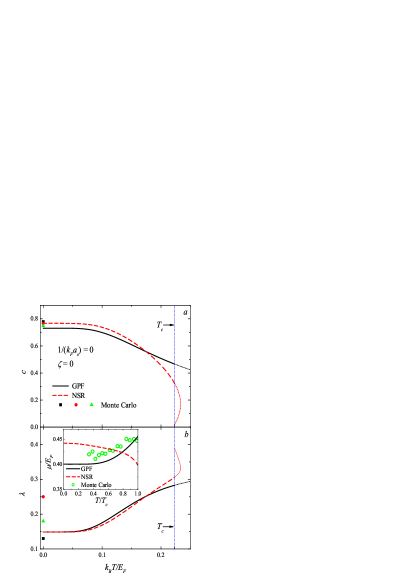
Figure 1: (color online) (a) Sound velocity parameter of the Bogoliubov–Anderson mode $c$ for cold fermions in 3D as a function of temperature in the unitarity regime and for $\zeta=0$. The parameters of state are determined taking into account the fluctuations in different ways: within the path-integral GPF formalism (solid curve) and within the NSR scheme (dashed curve). The symbols show the results of the different Monte Carlo calculations ^{14, 15, 16, 17, 18}. (b) The parameter $\lambda$ as a function of temperature in the same regime. The dot-dashed vertical line indicates the critical temperature of the superfluid phase transition. The thin dotted curves show the formal solutions for the parameter $c$ and $\lambda$ within the path-integral GPF and NSR approaches above $T_{c}$. Inset: Chemical potential calculated within the path-integral GPF and NSR approaches compared with the Monte Carlo data from Ref. ¹⁹.

In Fig. 1, the parameters $c$ and $\lambda$ characterizing pair excitations are plotted as a function of temperature for the balanced Fermi gas in the unitarity regime ($1/a_{s}=0$). The parameters of the equation of state for a given temperature are determined from the joint solution of the gap and number equations taking into account fluctuations in the number equation. The fluctuation contributions to the fermion density are calculated within the path-integral GPF and NSR schemes.

As found in Ref. ¹¹, the NSR approach becomes inaccurate in the vicinity of the critical temperature $T_{c}$. It was also shown that the NSR scheme reveals a re-entrant behavior of the parameters in the state above $T_{c}$, leading to an artificial first-order superfluid phase transition ²⁶. The re-entrant behavior of the parameters $c$ and $\lambda$ obtained in the NSR approach is clearly seen in Fig. 1. The critical temperature $T_{c}$ for the balanced gas, indicated by a dash-dotted line in Fig. 1, is the same within the NSR and GPF approaches. However, the GPF method leads to better results with respect to NSR for the broken-symmetry phase. This can be seen, for example, in the inset of Fig. 1 where we plot the chemical potential as a function of temperature below $T_{c}$ calculated within the NSR and path-integral GPF approaches and compared with the Monte Carlo results of Ref. ¹⁹.

In the zero-temperature limit, the sound velocity parameter $c$ for the pair excitations obtained within both the path-integral GPF and NSR approaches exhibits an excellent agreement with the numerical results obtained using different Monte Carlo algorithms ^{14, 15, 16, 17, 18}. Also the gradient parameter $\lambda$ at zero temperature lies within the range of the values of $\lambda$ obtained in Refs. ^{13, 25} as the best fitting parameters for the ground state energy of fermions compared with Monte Carlo data. This agreement demonstrates the accuracy of the present approach for the broken-symmetry phase of cold fermions.

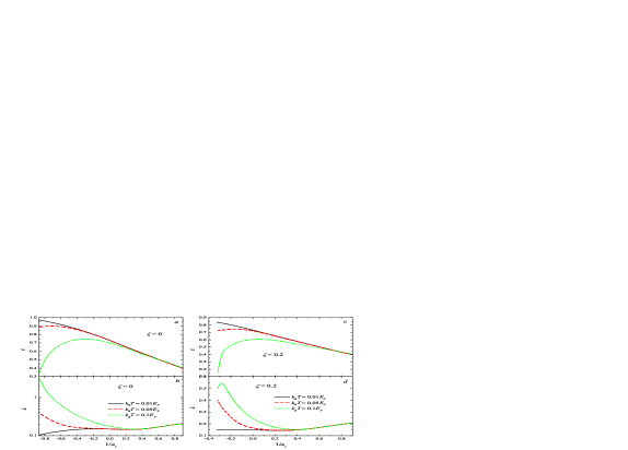
Figure 2: (color online) Sound velocity parameter (a, c) and parameter $\lambda$ (b, d) for the Bogoliubov–Anderson mode as a function of the inverse scattering length for $k_{B}T=0.01E_{F}$ (solid curves), for $k_{B}T=0.05E_{F}$ (dashed curves) and for $k_{B}T=0.1E_{F}$ (dotted curves) for a balanced Fermi gas (a, b) and at the chemical potential imbalance $\zeta=0.2$ (c, d) in the unitarity regime.

In Fig. 2, we plot the parameters $c$ and $\lambda$ as a function of the inverse scattering length $1/a_{s}$ for the balanced gas (the left-hand panels) and at the chemical potential imbalance $\zeta=0.2$ (the right-hand panels). At $k_{B}T=0.01E_{F}$ the sound velocity parameter monotonously decreases with increasing $1/a_{s}$. For non-zero temperatures, $c$ exhibits a maximum, which shifts to higher coupling strengths for higher temperatures. The parameter $\lambda$ at finite temperatures has a minimum, which almost vanishes in the zero-temperature limit. In the weak-coupling regime, both $c$ and $\lambda$ are sensitive to temperature. When moving towards the strong-coupling regime, $c$ and $\lambda$ gradually become almost independent on $T$. The imbalance leads to the appearance of a critical inverse scattering length such that for smaller $1/a_{s}$, there is no superfluid state (see, e. g., Ref. ²²).

3 Parameters of state

3.1 Thermodynamic functions

Using the spectra of the elementary fermionic and pair excitations derived in Sec. 2, we can obtain the thermodynamic functions of the superfluid Fermi gas at finite temperature. In Ref. ¹³, a similar description of the thermodynamic properties was performed for a unitary balanced Fermi gas using the zero-temperature spectra of elementary excitations.

In Ref. ¹³, a pair excitation spectrum of the form of expression (17) is used, where the zero-temperature sound velocity $c$ is taken from the Monte Carlo data ^{14, 15, 16, 17, 18} and the gradient parameter $\lambda$ is determined from a fit of the thermodynamic properties to the Monte Carlo results. In the present calculation, the pair excitation spectra are obtained using the analytic path-integral GPF approach without any fit.

In this section we consider the thermodynamic functions of the cold Fermi gas within the model of fermionic and pair excitations. The grand-canonical thermodynamic potential is the sum of the saddle-point and pair excitation contributions

$$\Omega=\Omega_{sp}+\Omega_{p}.$$ (20)

The saddle-point thermodynamic potential $\Omega_{sp}$ is given by Eq. (1). The contribution of pair excitations is ¹³

$$\Omega_{p}=\frac{V}{\beta}\int\frac{d\mathbf{q}}{\left(2\pi\right)^{3}}\ln\left(1-e^{-\beta\omega_{q}}\right).$$ (21)

The entropy $S$ is found using its relation to the grand-canonical thermodynamic potential,

$$S=-\left.\frac{\partial\Omega}{\partial T}\right|_{V,\mu,\zeta}.$$ (22)

Using the thermodynamic potential $\Omega$ with (1) and (21) we find that the entropy is expressed as

$$S =\frac{V\beta^{2}}{3\pi^{2}}\int_{0}^{\infty}\frac{\xi_{k}}{E_{k}}\frac{E_{k}\left(\cosh\beta E_{k}\cosh\beta\zeta+1\right)-\zeta\sinh\beta E_{k}\sinh\beta\zeta}{\left(\cosh\beta\zeta+\cosh\beta E_{k}\right)^{2}}k^{4}dk$$

$$+\frac{V}{2\pi^{2}}\int_{0}^{\infty}\left(\beta\omega_{q}\frac{e^{-\beta\omega_{q}}}{1-e^{-\beta\omega_{q}}}-\ln\left(1-e^{-\beta\omega_{q}}\right)\right)q^{2}dq.$$ (23)

Finally, the internal energy $E$ of cold fermions is calculated using the relation between $E$ and the grand-canonical thermodynamic potential, $E=\Omega+TS+\mu N,$where $N$ is the total number of fermions.

In Fig. 3, the internal energy per particle for a unitary Fermi gas calculated in different approaches is plotted as a function of temperature for the broken-symmetry phase at $T\leqslant T_{c}$. The critical temperature determined within the path-integral GPF model is the same as within NSR, $T_{c}\approx 0.225E_{F}/k_{B}$. The results of the present calculation within the model of fermionic and low-lying pair excitations with parameters determined using the path-integral GPF and NSR methods are shown with short-dashed and dot-dashed curves, respectively. The other results represented in Fig. 3 are (after Ref. ¹³): the internal energy calculated within the low-temperature fermion-boson (FB) model ¹³, and the result of the analytic model proposed by Bulgac, Drut, and Magierski (BDM) ¹⁹. The analytic results are compared with those of the Monte Carlo calculations from Ref. ¹⁹ and with the experimental data of Ref. ²⁷ for a gas of ⁶Li atoms at unitarity.

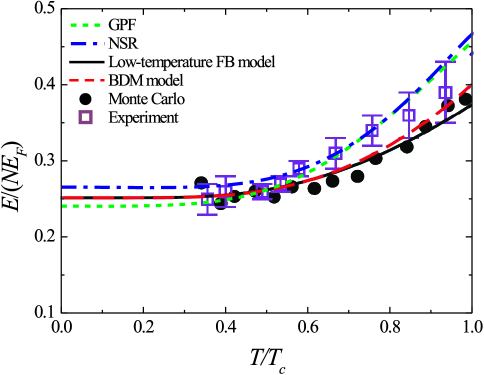
Figure 3: (color online) Internal energy per particle for a Fermi gas at unitarity calculated within the model of fermionic and low-lying pair excitations with parameters determined using the path-integral GPF method (short-dashed curve) and the NSR theory (dot-dashed curve). The solid curve shows the internal energy obtained within the low-temperature fermion-boson model in Ref. ¹³. The dashed curve is the result of the BDM model ¹⁹. The full dots represent the Monte Carlo simulations ¹⁹. The squares are the experimental data ²⁷.

As reported in Ref. ¹³, the low-temperature fermion-boson model works well in the broken-symmetry phase where the internal energy resulting from this model is close to the Monte Carlo data of Ref. ¹⁹. The present study is performed with the parameters of the elementary excitations obtained using the analytic approaches rather than a fit to the Monte Carlo simulations. The internal energy calculated in the present work with the parameters determined using the path-integral GPF method is very close to the Monte Carlo results at low temperatures $T\lessapprox 0.55T_{c}$. Furthermore, our result is in good agreement with the experiment ²⁷ in the whole temperature range below $T_{c}$.

Neither the model of fermionic and pair excitations used in the present work, nor the low-temperature fermion-boson model of Ref. ¹³ predicts the superfluid phase transition: the critical temperature $T_{c}$ is determined within the path-integral GPF method before the long-wavelength expansion is performed in Sec. 2. However, the latter model can describe well the broken-symmetry phase of cold fermionic atoms.

3.2 Superfluid density

The total density of cold fermions within the model of fermionic and pair excitations is given by the sum of fermion and boson contributions

$$n=\frac{1}{2\pi^{2}}\int_{0}^{\infty}k^{2}dk\left(1-\frac{\xi_{k}}{E_{k}}X_{k}\right)+\frac{1}{\pi^{2}}\int_{0}^{\infty}q^{2}dq\frac{1}{e^{\beta\omega_{q}}-1}.$$ (24)

The total density is a sum of the normal and superfluid densities $n=n_{n}+n_{s}$. The superfluid density $n_{s}$, as well as the total density, is constituted by the saddle-point result for an imbalanced Fermi gas and the contribution due to the pair excitations,

$$n_{s} =\frac{1}{2\pi^{2}}\int_{0}^{\infty}\left(1-\frac{\xi_{k}}{E_{k}}X_{k}-k^{2}Y_{k}\right)k^{2}dk$$

$$+\frac{1}{\pi^{2}}\int_{0}^{\infty}\left(\frac{1}{e^{\beta\omega_{q}}-1}-\frac{\beta}{3}q^{2}\frac{e^{-\beta\omega_{q}}}{\left(e^{-\beta\omega_{q}}-1\right)^{2}}\right)q^{2}dq,$$ (25)

where the function $Y_{k}$ is given by

$$Y_{k}\equiv\frac{\partial X_{k}}{\partial E_{k}}=\beta\frac{\cosh\beta E_{k}\cosh\beta\zeta+1}{\left(\cosh\beta E_{k}+\cosh\beta\zeta\right)^{2}}$$

(see the analogous expression for the Fermi gas in 2D in Ref. ²⁸). In the balanced case, the superfluid density becomes equivalent to the corresponding expression of Ref. ¹³, but with other values of the parameters of the pair excitations, as discussed above and shown in Fig.1.

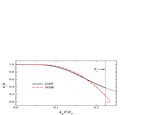
Figure 4: (color online) Superfluid density for a Fermi gas at unitarity calculated within the model of fermionic and pair excitations with parameters determined using the path-integral GPF method (solid curve) and the NSR theory (dashed curve). Thin dotted curves correspond to the temperature range above $T_{c}$.

In Fig. 4, the superfluid density divided by the total density calculated within the model of fermionic and pair excitations is plotted as a function of temperature. As seen from the figure, the superfluid density calculated using the parameters of the pair excitations obtained within the NSR model exhibits a re-entrant behavior above $T_{c}$ similarly to the sound velocity parameter in Fig. 1. The analogous bend-over of the superfluid density above $T_{c}$ was reported in the full NSR approach in Ref. ²⁶.

3.3 Sound velocities

We consider the sound propagation in a superfluid Fermi gas using the approach of the two-fluid hydrodynamics ^{29, 30} in the same way as in Ref. ¹³. The first sound velocity $u_{1}$ in the two-fluid hydrodynamics is determined by the formula

$$u_{1}=\left(2\left.\frac{\partial P}{\partial n}\right|_{\bar{S},V}\right)^{1/2},$$ (26)

with the entropy per particle $\bar{S}=S/N$. The pressure is proportional to the grand-canonical thermodynamic potential: $P=-\Omega/V$. We adopt the expression ³¹

$$\left.\frac{\partial P}{\partial n}\right|_{\bar{S},V}=\frac{5}{3}\frac{P}{n}$$ (27)

and use the grand-canonical thermodynamic potential given by Eq. (20) with (1) and (21).

The second sound velocity $u_{2}$ characterizes the temperature waves in which the motion of the normal and superfluid fractions is out-of-phase. It is determined by the formula

$$u_{2}=\left(\frac{2\bar{S}^{2}}{\left.\frac{\partial\bar{S}}{\partial T}\right|_{N,V}}\frac{n_{s}}{n_{n}}\right)^{1/2}.$$ (28)

The formulae (26) and (28) are valid as far as the first-sound and second-sound modes are decoupled. Following Ref. ¹³, we assume that the above condition is fulfilled for a cold Fermi gas.

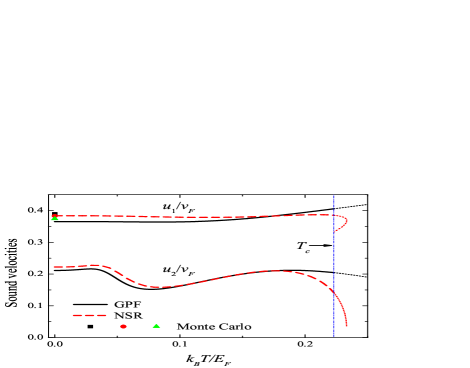
Figure 5: (color online) First and second sound velocities for a unitary Fermi gas calculated within the model of fermionic and pair excitations with parameters determined using the path-integral GPF method (solid curves) and the NSR theory (dashed curves). The symbols show the Monte Carlo results for the first sound velocity. Thin dotted curves correspond to the temperature range above $T_{c}$.

In Fig. 5, the first and second sound velocities (divided by the zero-temperature Fermi velocity $v_{F}$) are plotted as a function of temperature. They are calculated within the model of fermionic and pair excitations using the parameters of pair excitations determined by the path-integral GPF and NSR methods.

The first and second sound velocities obtained using the model of fermionic and pair excitations are in a reasonable agreement with the results of the analysis based on the full NSR thermodynamics ^{31, 32}. In the zero-temperature limit, the first sound velocity tends to the same limit as the sound velocity parameter $c$ for pair excitations, which is extremely close to the Monte Carlo data ^{14, 15, 16, 17, 18}.

4 Conclusions

In the present work, the GPF modification ^{11, 12} of the NSR scheme has been formulated in the path-integral representation and extended to the case of imbalanced fermions. Within this path-integral GPF approach, we have analytically derived the spectra of low-lying pair excitations of the imbalanced Fermi gas with $s$-wave pairing at finite temperatures and extracted the parameters $c$ and $\lambda$ for the pair excitations from these results. Using these spectra, the finite-temperature thermodynamics of the Fermi gas in the superfluid state has been analyzed. The obtained internal energy demonstrates a good agreement with the Monte Carlo results and is remarkably close to the experimental data for the Fermi gas at unitarity. The zero-temperature value of the first sound velocity is in a good agreement with the results of the Monte Carlo simulations. The present method allows us to obtain the spectra of the elementary excitations and, consequently, the thermodynamic parameters of the state for an arbitrary scattering length, at non-zero temperatures, and for non-zero imbalance.