Mesoscopic Current-In-Plane Giant Magneto-Resistance

Abstract

We develop a three dimensional semiclassical theory which generalizes the Valet-Fert model in order to account for non-collinear systems with magnetic texture, including e.g. domain walls or magnetic vortices. The theory allows for spin transverse to the magnetization to penetrate inside the ferromagnet over a finite length and properly accounts for the Sharvin resistances. For ferromagnetic-normal-ferromagnetic multilayers where the current is injected in the plane of the layers (CIP), we predict the existence of a non zero mesoscopic CIP Giant Magneto-Resistance (GMR) at the diffusive level. This mesoscopic CIP-GMR, which adds to the usual ballistic contributions, has a non monotonic spatial variation and is reminiscent of conductance quantization in the layers. Furthermore, we study the spin transfer torque in spin valve nanopillars. We find that when the magnetization direction is non uniform inside the free layer, the spin torque changes very significantly and simple one-dimensional calculations cease to be reliable.

Quantum effects in electronic transport are usually small deviations to the classical Ohm’s law. Famous examples include weak localization corrections Anderson et al. (1979); Gorkov et al. (1979) and universal conductance fluctuations Altshuler (1985); Lee and Stone (1985) which can be observed in diffusive systems. On the other hand, in small mesoscopic systems quantum mechanics can lead to an entirely different behavior of the conductance. Perhaps the most paradoxical example is the case of a smooth nanoconstriction in a two dimensional electron gas (quantum point contact) where by varying the strength of the confinement the conductance variation has a step-like character with plateaus quantized in unit of $2e^{2}/h$ van Wees et al. (1988); Wharam et al. (1988). This observation was at first a bit puzzling since the quantum point contact does not have any source of scattering, neither elastic nor inelastic. The crucial concept for clarifying the picture was the notion of reservoirs (electrodes) attached to the quantum point contact where the energy relaxation takes place.

We revisit bellow this issue in the context of the Giant Magnetoresistance (GMR) effect Baibich et al. (1988); Binasch et al. (1989) observed in magnetic multilayers comprising ferromagnetic layers (${\rm F}$) separated by a normal metal (${\rm N}$) structures. We consider ${\rm F|N|F}$ trilayer spin valve structure. There exist two geometries for GMR. In the CPP geometry one injects the current perpendicular to the plane Pratt et al. (1991); Bass and Pratt (1999); Piraux et al. (1994) of the layers. The CPP-GMR can be understood simply within a two-current model where electrons with up and down spins experience different resistances as they cross the two magnetic layers. As a result, the configuration where the magnetizations of the FM layers are parallel (P) has a different resistance from the anti-parallel (AP) one, hence giving rise to the GMR. However, the original experiments Baibich et al. (1988); Binasch et al. (1989); Parkin et al. (1990); Parkin (1995) were performed in CIP geometry where one injects the current within the plane (CIP) of the layers. The CIP setup is much simpler experimentally but the two current model (as well as its generalization, the Valet-Fert Valet and Fert (1993) drift diffusion theory) predicts a vanishing GMR. This usually complicates the interpretation of the experiments as one needs to introduce (sub mean free path quantum) microscopic approaches and the resulting GMR can be quite sensitive to the details of the model ( Camley and Barnaś (1989); Levy et al. (1990); Vedyayev et al. (1993, 1997, 1998) and references therein). Here, we predict the existence of an additional contribution to CIP-GMR which already exists at the drift-diffusion level. This contribution has the same origin as the quantification of conductance and should dominate the usual ballistic contributions for mesoscopic systems.

In this work we address the following problems. First, a physical explanation for the role of conductance quantization in CIP-GMR is provided. Next, we develop a theoretical framework allowing for a quantitative prediction of this effect. This framework which we refer to as Continuous Random Matrix Theory in $3$ Dimensions (CRMT3D) extends on a previous one dimensional semi-classical approach CRMT and goes beyond existing models Strelkov et al. (2010). Finally, we apply CRMT3D to the study of the spin transfer torque effect in a CPP nanopillar.

I Sharvin resistance and CIP-GMR: physical picture.

A very transparent way to describe transport in a quantum system is the Landauer-Bü ttiker formalism Büttiker (1986) where one describes quantum transport with a scattering matrix that relates the amplitudes of outgoing to the incoming modes. The quantum system is treated as a waveguide with $N_{\rm ch}\sim A/\lambda_{F}^{2}$ propagating modes. In the metallic systems considered here, their cross section $A$ is much larger than the square of the Fermi wave length $\lambda_{F}$, so they typically contain thousands of conducting channels. The Landauer formula relates the transmission probability $T_{n}$ of channel $n$ with the conductance as $g={e^{2}/h}\sum_{n=1}^{N_{\rm ch}}T_{n}$ so that for a perfectly transparent system ($T_{n}=1$) the system has a finite Sharvin resistance Sharvin (1965) ${\cal R}_{\rm sh}=h/(N_{\rm ch}e^{2})$ . As mentioned above, the Sharvin resistance (also known as contact resistance) has been observed repeatedly, in particular in semiconductor based mesoscopic systems where $N_{\rm ch}$ can be tuned with the help of an electric field. The Sharvin resistance needs to be accounted for only once: when two systems $A$ and $B$ (of resistances ${\cal R}_{A}$ and ${\cal R}_{B}$) are connected in series, the total resistance is given (in the many channels limit $N_{\rm ch}\gg 1$ considered here) byDatta (1997); Rychkov et al. (2009) ${\cal R}_{AB}={\cal R}_{A}+{\cal R}_{B}-{\cal R}_{\rm sh}$. In other words one adds up the intrinsic resistances ${\cal R}_{A}-{\cal R}_{\rm sh}$ of the conductors in series (regular Ohm’s law) and adds once a contact ${\cal R}_{\rm sh}/2$ resistor for each electrode. For metallic spin valves under consideration here, the Sharvin resistance is the leading quantum correction to Ohm’s law. ${\cal R}_{\rm sh}$ typically corresponds to the resistance of an interface between two different metals or, say, 10 nm of bulk material. This resistance would normally be difficult to distinguish from a series resistance coming from the measuring apparatus. However, we shall see that in the case of the CIP geometry, the GMR signal simply vanishes at the purely classical level (more precisely in the limit of validity of the Valet-Fert model Valet and Fert (1993) described below) and the presence of the Sharvin (quantum) resistance provides the leading source of GMR of mesoscopic samples.

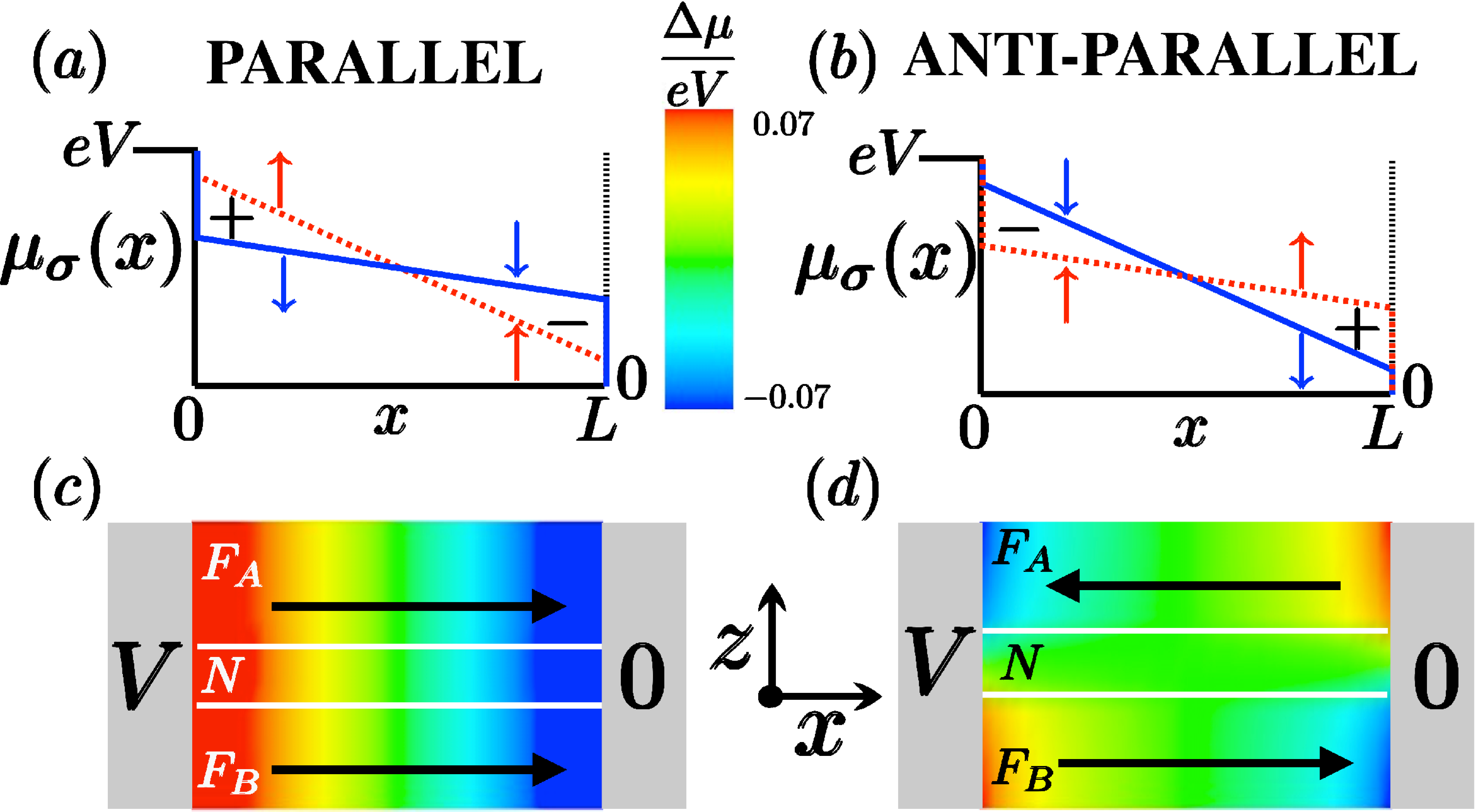
Figure 1: Upper panels: Cartoon of the spin resolved chemical potential (up spins: dotted line, down spins: full line) of the top layer of a CIP-GMR setup as a function of the position $x$ in between the electrodes. The chemical potentials drop from $eV$ ($x=0$) to $0$ ($x=L$). The initial and final drop at $x=0/L$ is due to the presence of the Sharvin resistances. Lower panels: numerical simulations of spin accumulation in a ${\rm Co_{3}|Ag_{1}|Co_{3}}$ trilayer with a size $L=20nm$. Left (a,c) and Right (b,d) panels correspond respectively to the parallel and anti parallel configurations.

The proper generalization of Ohm’s law to a three dimensional magnetic multilayer stack is given by the Valet-Fert equations:

$${\bf j}_{\sigma} = -\frac{1}{e\rho_{\sigma}}\boldsymbol{\nabla}\boldsymbol{\mu}_{\sigma}$$ (1)

$$\boldsymbol{\nabla}\cdot{\bf j}_{\sigma} = \frac{1}{e\rho_{\sigma}\ell_{\rm sf}^{2}}\left[\boldsymbol{\mu}_{-\sigma}-\boldsymbol{\mu}_{\sigma}\right],$$ (2)

where Eq.(1) is Ohm’s law relating the spin resolved current ${\bf j}_{\sigma}$ to the gradient of the spin resolved chemical potential $\boldsymbol{\mu}_{\sigma}$ with the spin dependent resistivity $\rho_{\sigma}$. Eq. (2) expresses the (lack of) conservation of spin current: the divergence of spin current is balanced by spin relaxation which is proportional to the spin accumulation $\boldsymbol{\Delta\mu}=\boldsymbol{\mu}_{\uparrow}-\boldsymbol{\mu}_{\downarrow}$ and controlled by the spin diffusive length $\ell_{\rm sf}$.

A cartoon of the system is presented in the lower panel of Fig. 1: it consists of two magnetic layers $F_{A}$ and $F_{B}$ separated by a normal spacer $N$ and connected sideways to the two electrodes to which a voltage $V$ is applied. To elucidate the role of Sharvin resistances in CIP-GMR, let us first ignore the role of spin-flip processes. In the absence of Sharvin resistances, one finds that the spin dependence of the resistivity in the magnetic layers is essentially irrelevant: the chemical potential must drop linearly from $eV$ at $x=0$ to $0$ at $x=L$ irrespectively of the values of the resistivities $\rho_{\sigma}$. As a result, $\boldsymbol{\mu}_{\sigma}(x,z)$ is constant along the growth $z$ direction and there is no current flow along $z$. There is neither spin accumulation in the system nor GMR. The same conclusion can be drawn from a full analysis of the Valet-Fert equations. The situation changes drastically when the system is connected in series with its contact (Sharvin) resistances as schematically sketched in Fig. 1 (a) and (b): for an electron species (say majority electron) with low resistivity ($\rho_{\sigma}L\ll{\cal R}_{\rm sh}$) the chemical potential drops mostly at the contacts while for an electron species (say minority electron) with large resistivity ($\rho_{\sigma}L\gg{\cal R}_{\rm sh}$) most of the drop takes place in the bulk. As a result some spin accumulation builds up in the system. In particular, in the AP configuration, the up spin (for example) chemical potential varies along the $z$ direction leading thereby to some spin current flow along the $z$ axis. The current patterns become different for P and AP configurations and the GMR is restored. The color code of the lower panels of Fig. 1 represents the spin accumulation profile calculated $\boldsymbol{\Delta\mu}$ for a ${\rm Co_{3}|Ag_{1}|Co_{3}}$ (thicknesses in $nm$) trilayer using the theoretical approach described in the following section. We observe a clear non zero spin accumulation in Fig. 1 (c) and (d) for a CIP geometry. This effect is a direct consequence of the presence of non negligible quantum contact resistances.

II 3D Semi-classical theory : CRMT3D.

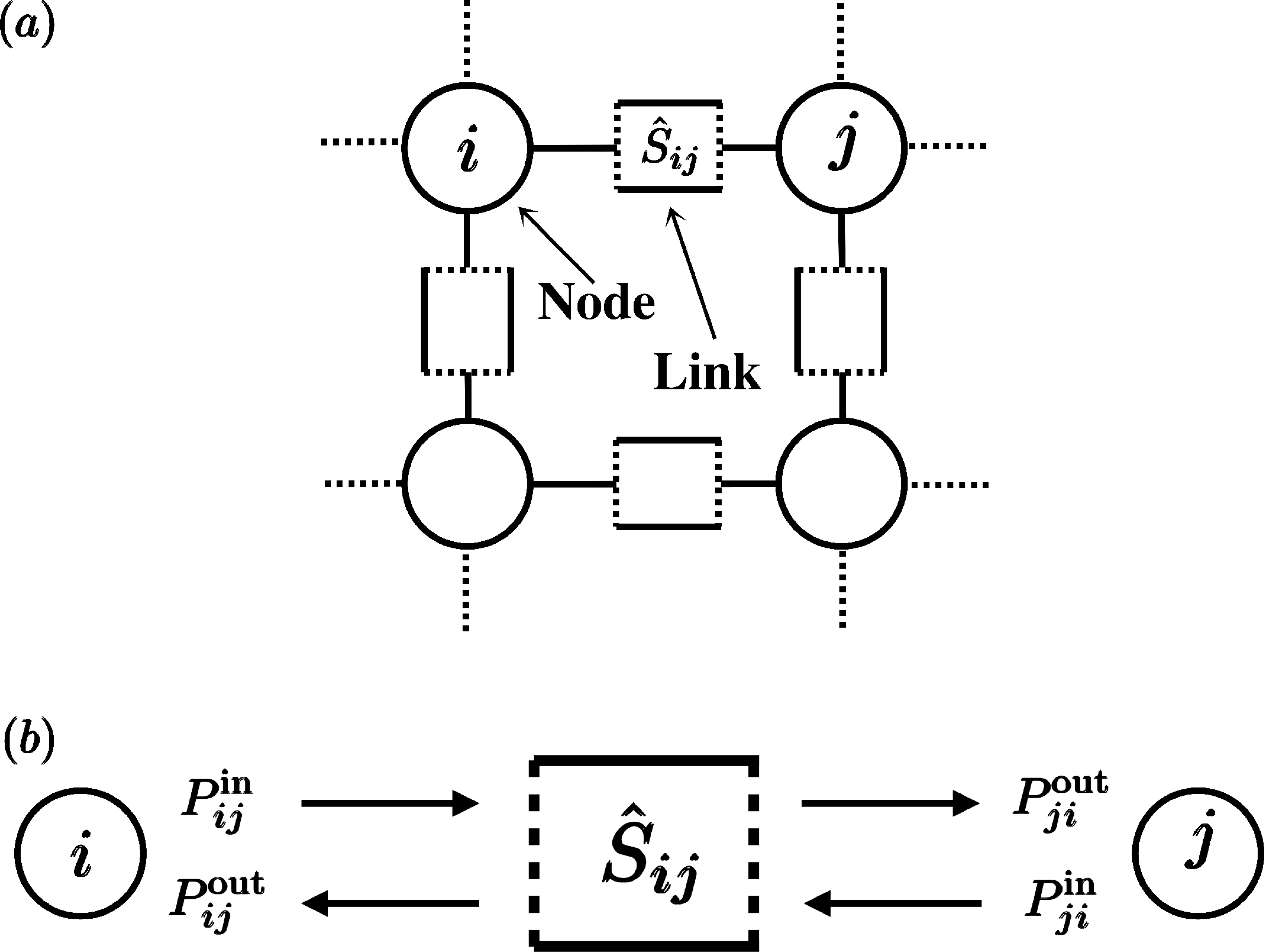
Figure 2: Panel (a) is a cartoon of discretization of the systems in nodes connected by links. Each node is labeled by a latin index ($i$, $j$,…) and a link by the two latin indices of the associated nodes. Panel (b) is a cartoon of the Scattering matrix $\hat{S}_{ij}$. We define the region $i$ on the left and $j$ on the right. The ${\rm in}$ (${\rm out}$) stands for incoming (outgoing) probabilities mode ${\bf P}^{\rm in/out}_{ij}$, where the first index correspond to the side on which the probability current is defined.

In order to provide a quantitative description of aforementioned effects and to capture situations where the magnetization has a non-trivial texture (domain walls, vortices…), we develop a full 3D semi-classical theory hereafter referred to as CRMT3D. This approach can be viewed as a generalization of the 3D Valet-Fert theory that properly accounts for Sharvin resistances and non-collinear situations. In addition, CRMT3D can also be considered as a continuous version of the generalized circuit theory Bauer et al. (2003) or equivalently of the random matrix theory developed in Ref. [Waintal et al., 2000]. CRMT3D is a straightforward generalization of the recently developed CRMT (Continuous Random Matrix Theory) for unidimensional systems Rychkov et al. (2009); Borlenghi et al. (2011). We refer to Refs. [Rychkov et al., 2009; Borlenghi et al., 2011] for a full derivation of the one dimensional CRMT theory. For completeness, we recall below the basic objects of the theory before extending it to three dimensions.

A schematic cartoon of the structure of CRMT3D is presented in Fig. 2(a) where the system is discretized into many nodes of small volume. Here we choose a simple Cartesian mesh but this choice is not compulsory. The nodes are connected to their neighbors by links. This set of nodes and links forms a circuit theory entirely equivalent to the so called generalized circuit theory Bauer et al. (2003); Rychkov et al. (2009). The theory has four basic variables per link $ij$: ${\bf P}^{\rm out}_{ij}$, ${\bf P}^{\rm in}_{ij}$, ${\bf P}^{\rm out}_{ji}$ and ${\bf P}^{\rm in}_{ji}$ where the labels in (out) refer to currents going from (to) the nodes while the index order $ij$ ($ji$) indicates that the probability current is defined on node $i$ (node $j$) side as sketched in Fig. 2(b). The probability currents

$${\bf P}_{ij}=\left(\begin{array}[]{l}P_{ij,\uparrow}\\ P_{ij,{\rm mx}}\\ P^{\rm\,\ast}_{ij,{\rm mx}}\\ P_{ij,\downarrow}\end{array}\right)$$ (3)

are $4$-vectors that encapsulate the current probabilities for majority ($P_{ij,\uparrow}$ ) and minority ($P_{ij,\downarrow}$ ) electrons as well as spin currents transverse to the magnetization of the layer ($P_{ij,{\rm mx}}$). The theory is defined by two fundamental equations relating the outgoing to the incoming currents: one for the links and one for the node.

The link equation is identical to its counterpart in one dimension:

$$\begin{pmatrix}{\bf P}^{\rm out}_{ij}\\ {\bf P}^{\rm out}_{ji}\end{pmatrix}=\hat{S}_{ij}\begin{pmatrix}{\bf P}^{\rm in}_{ij}\\ {\bf P}^{\rm in}_{ji}\end{pmatrix},$$ (4)

where the Scattering matrix $\hat{S}_{ij}$

$$\hat{S}_{ij}=\left(\begin{array}[]{cc}\hat{r}^{\prime}&\hat{t}\\ \hat{t}^{\prime}&\hat{r}\end{array}\right),$$ (5)

is composed of $4\times 4$ transmission $\hat{t}$, $\hat{t}^{\prime}$ and reflection $\hat{r}$, $\hat{r}^{\prime}$ material dependent subblocks. The $\hat{S}_{ij}$ matrix of a thin slice of material of width $b$ is parametrized by two matrices $\Lambda^{t}$ and $\Lambda^{r}$:

$$\hat{t}=1-\Lambda^{t}\,b,\quad\hat{r}=\Lambda^{r}\,b.$$ (6)

Finally, the matrices $\Lambda^{t}$ and $\Lambda^{r}$ of a ferromagnetic metal are parametrized by four independent parameters ($\Gamma_{\uparrow}$, $\Gamma_{\downarrow}$, $\Gamma_{{\rm sf}}$, $\Gamma_{{\rm mx}}$) and read,

$$\Lambda^{t}= \!\!\!\!\!\!\!\!\left(\begin{array}[]{cccc}\Gamma_{\uparrow}+\frac{1}{d}\,\Gamma_{\rm sf}&0&0&-\frac{1}{d}\,\Gamma_{\rm sf}\\ 0&\frac{1}{d}\Gamma_{\rm mx}&0&0\\ 0&0&\frac{1}{d}\,\Gamma^{\,\ast}_{\rm mx}&0\\ -\frac{1}{d}\,\Gamma_{\rm sf}&0&0&\Gamma_{\downarrow}+\frac{1}{d}\,\Gamma_{\rm sf}\end{array}\right),$$ (11)

$$\Lambda^{r}= \!\!\!\!\!\!\!\!\left(\begin{array}[]{cccc}\Gamma_{\uparrow}-\frac{1}{d}\,\Gamma_{\rm sf}&0&0&\frac{1}{d}\,\Gamma_{\rm sf}\\ 0&0&0&0\\ 0&0&0&0\\ \frac{1}{d}\,\Gamma_{\rm sf}&0&0&\Gamma_{\downarrow}-\frac{1}{d}\,\Gamma_{\rm sf}\end{array}\right),$$ (16)

where $d=3$ is the spatial dimension. As expected, for a unidimensional system ($d=1$) Eqs. (11,16) reduce to the one obtained in the CRMT approach, Eqs.(36,37) of Ref. [Borlenghi et al., 2011]. The meaning of the parameters are also identical and thus linked to $5$ physical lengths : the spin resolved mean free path $\ell_{\sigma}=1/\Gamma_{\sigma}$, the spin diffusion length $\ell_{\rm sf}=[4\Gamma_{\rm sf}(\Gamma_{\uparrow}+\Gamma_{\downarrow})]^{-1/2}$, the transverse spin penetration length $\ell_{\perp}$ and the Larmor precession length $\ell_{\rm L}$. The two latter are encoded into the complex number $\Gamma_{\rm mx}=1/\ell_{\perp}+i/\ell_{\rm L}$. Note that although the role of $\ell_{\perp}$ and $\ell_{\rm L}$ can lead to interesting physics, in the numerical simulations performed in this paper, we restrict ourself to situations where these lengths are very small (sub nanometer) so that spin torques essentially develop at the normal metal-ferrromagnet interface. For a normal material, we substitute in Eqs. (11), $\Gamma_{\sigma}\Rightarrow\Gamma$ and $\frac{1}{d}\Gamma_{\rm mx}\Rightarrow\Gamma+\frac{2}{d}\,\Gamma_{\rm sf}$ so that $\Lambda^{t}$ remains invariant upon arbitrary rotation of the spin quantization axis. $\Lambda^{r}$ is obtained by following the same procedure but with $\Gamma_{\rm sf}$ replaced by $-\Gamma_{\rm sf}$. The scattering matrices describing the interface between two metals are strictly identical to those developed in the one dimensional CRMT case to which we refer for their expression (See section E of Ref. Borlenghi et al., 2011 for details).

Although the natural variables of the theory are the probabilities ${\bf P}^{\rm in/out}_{ij}$, they are intrinsically related to the spin resolved chemical potential

$${\boldsymbol{\mu}}_{ij}=\frac{1}{2}\left[{\bf P}^{\rm in}_{ij}+{\bf P}^{\rm out}_{ij}\right]$$ (17)

and the spin resolved currents

$${\bf j}_{ij}=\frac{1}{e{\cal R}_{\rm sh}}\left[{\bf P}^{\rm in}_{ij}-{\bf P}^{\rm out}_{ij}\right]$$ (18)

flowing from $i$ to $j$. The equation at the node is obtained by enforcing two conditions. First the chemical potential $\boldsymbol{\mu}_{i}$ depends on $i$ only (and not on the link $ij$):

$$\boldsymbol{\mu}_{i}\equiv{\boldsymbol{\mu}}_{ij},\,\forall j\in Z_{i},$$ (19)

where $Z_{i}$ is the set of neighbors of node $i$. Second, the current is conserved at each node,

$$\sum_{j\in Z_{i}}{\bf j}_{ij}={\bf j}^{\rm src}_{i},$$ (20)

where the source term ${\bf j}^{\rm src}_{i}$ is present only for the nodes connected to electrodes. It is simply given by

$${\bf j}^{\rm src}_{i}=\frac{1}{e{\cal R}_{\rm sh}}{\boldsymbol{\mu}}^{\rm src}_{i}\quad\mbox{with,}\quad{\boldsymbol{\mu}}^{\rm src}_{i}=\begin{pmatrix}eV_{a}\\ 0\\ 0\\ eV_{a}\end{pmatrix},$$ (21)

where $V_{a}$ is the voltage imposed at the electrode $a$. Rewriting Eqs. (19,20) in terms of probabilities and substituting $\boldsymbol{\mu}_{i}$, Eq. (17) yields the node equation,

$${\bf P}^{\rm in}_{ij}=-{\bf P}^{\rm out}_{ij}+\frac{2}{|Z_{i}|}\sum_{j\in Z_{i}}{\bf P}^{\rm out}_{ij}+\frac{2}{|Z_{i}|}{\boldsymbol{\mu}}^{\rm src}_{i},$$ (22)

where $|Z_{i}|$ is the total coordination number of the node $i$ (counting the connections to other nodes plus the possible presence of a connected electrode). The set of Eq.(4), Eq.(21) and Eq.(22) fully defines the theory. It is equivalent by construction to CRMT for one dimensional case and one easily verify that taking the continuous limit of Eqs. (17,18) for collinear system, one recovers the VF equations Eqs. (1,2). CRMT3D can be used in a variety of ways, both analytical and numerical. A very efficient numerical solution (used in the next section for up to a million nodes) consists of simply iterating the set of equations (4), (21) and (22) from an arbitrary starting point until until convergence.

III Numerical results for CIP-GMR.

We now apply CRMT3D to CIP-GMR. We perform our simulations on various stacks on square samples of size $L\times L$. A typical result is presented in Fig. 3 where the GMR defined as GMR$=({\cal R}_{\rm AP}-{\cal R}_{\rm P})/({\cal R}_{\rm AP})$ is plotted as a function of $L$ for several ${\rm F|N|F}$ structures. Here $R_{\rm P}$ and $R_{\rm AP}$ represent the resistance in the $P$ and $AP$ configurations, respectively. The GMR vanishes in two limiting cases: (i) when $L\ll\min(\ell_{\uparrow},\ell_{\downarrow})$, the resistance is entirely dominated by the Sharvin resistance which does not depend on spin; (ii) when $L\gg\max(\ell_{\uparrow},\ell_{\downarrow})$ the resistance is dominated by the Ohmic resistance and spin accumulation vanishes as discussed above. Hence, one observes a negative correction for GMR (typically $-1\%$) for sizes $L\sim\ell_{\sigma}$ (i.e. when intrinsic and Sharvin resistances have comparable contributions). The actual value of the GMR depends on the kind of material considered (as shown Fig. 3) and the various thicknesses of the layers. For instance, weakly resistive normal metals such as the copper ${\rm Cu}$ (blue squares and green triangles in Fig. 3) favors a shunting effect through the spacer which reduces the mesoscopic GMR signal.

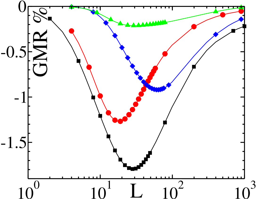
Figure 3: Numerical simulations of CIP-GMR (percent) as a function of the system size $L$ for various ${\rm F|N|F}$ trilayers: ${\rm Co_{3}|Ag_{1}|Co_{3}}$ (Black squares), ${\rm Py_{3}|Ag_{1}|Py_{3}}$ (red circles), ${\rm Py_{3}|Cu_{1}|Py_{3}}$ (blue diamonds) and ${\rm Co_{3}|Cu_{1}|Co_{3}}$ (green triangles).

In addition, we note the following characteristics: (i) We expect that raising the temperature has opposite effects on the two sides of the negative peak. Indeed, when raising the temperature the effective mean free paths (which includes both elastic and inelastic scattering) decreases. This makes the Sharvin contribution even less significant for large systems so that the GMR decreases in magnitude. However, for very small systems where the Sharvin contribution dominates, the GMR will start to build up. (ii) The sign of the effect effect is opposite to the CPP case: in the AP configuration, the minority electrons of one layer take advantage of the CIP configuration to propagate more freely in the other layer. (iii) One should keep in mind that this effect occurs in addition to other microscopic ballistic contributions (typically a few to ten $\%$). Parametrically, this mesoscopic CIP-GMR vanishes algebrically as $1/(1+L/\ell_{\sigma})$ while ballistic contributions decay exponentially $e^{-l_{\rm N}/\ell_{\sigma}}$ with the width $l_{\rm N}$ of the normal spacer. It is therefore possible to see the mesoscopic effect only but for most stacks one would observe both effects simultaneously and mesoscopic CIP-GMR should therefore be observed as a dip in the $L$ dependence of GMR.

Measuring the size dependence of CIP-GMR is not an easy experimental task. However, a very similar signature can be obtained by measuring the (two-terminal) GMR using a STM tip as a function of the distance between the tip and the contact electrode. The setup is presented in the inset of Fig. 4 where the tip is placed on top of the stack at a voltage $V$ while the two other electrodes are grounded. It corresponds to a geometry and sizes very similar to those used in the low temperature STM experiment of Ref. Sueur et al. (2008). As the distance $x$ between the tip and the contact electrode increases, the GMR is anticipated to change from positive (CPP like) to negative when the mesoscopic CIP GMR effects dominates.

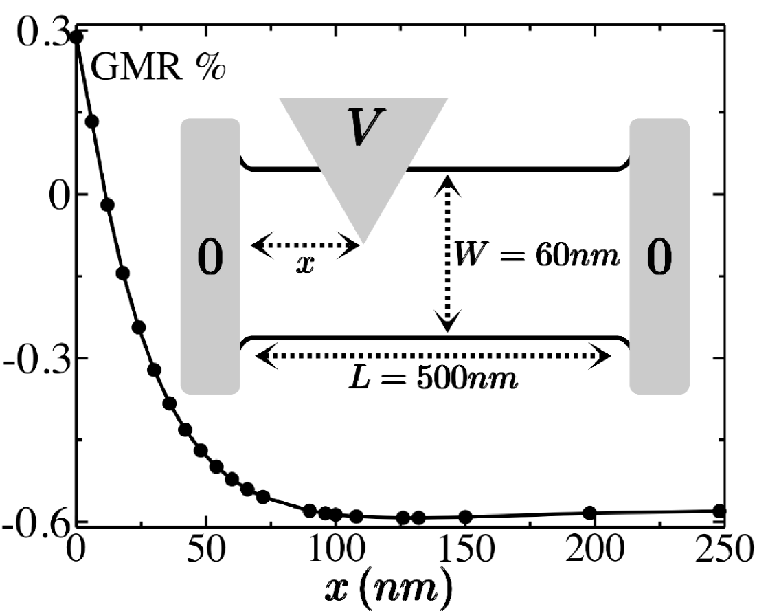
Figure 4: mesoscopic GMR in percent as function of the STM position $x$ for a ${\rm F|N|F}$ trilayers: ${\rm Co_{2}|Ag_{2}|Co_{2}}$, with a length $L=500nm$ and a width $W=60nm$. Inset: Cartoon of the top view of the setup.

IV Conclusion: spin-torque in a realistic CPP spin valve.

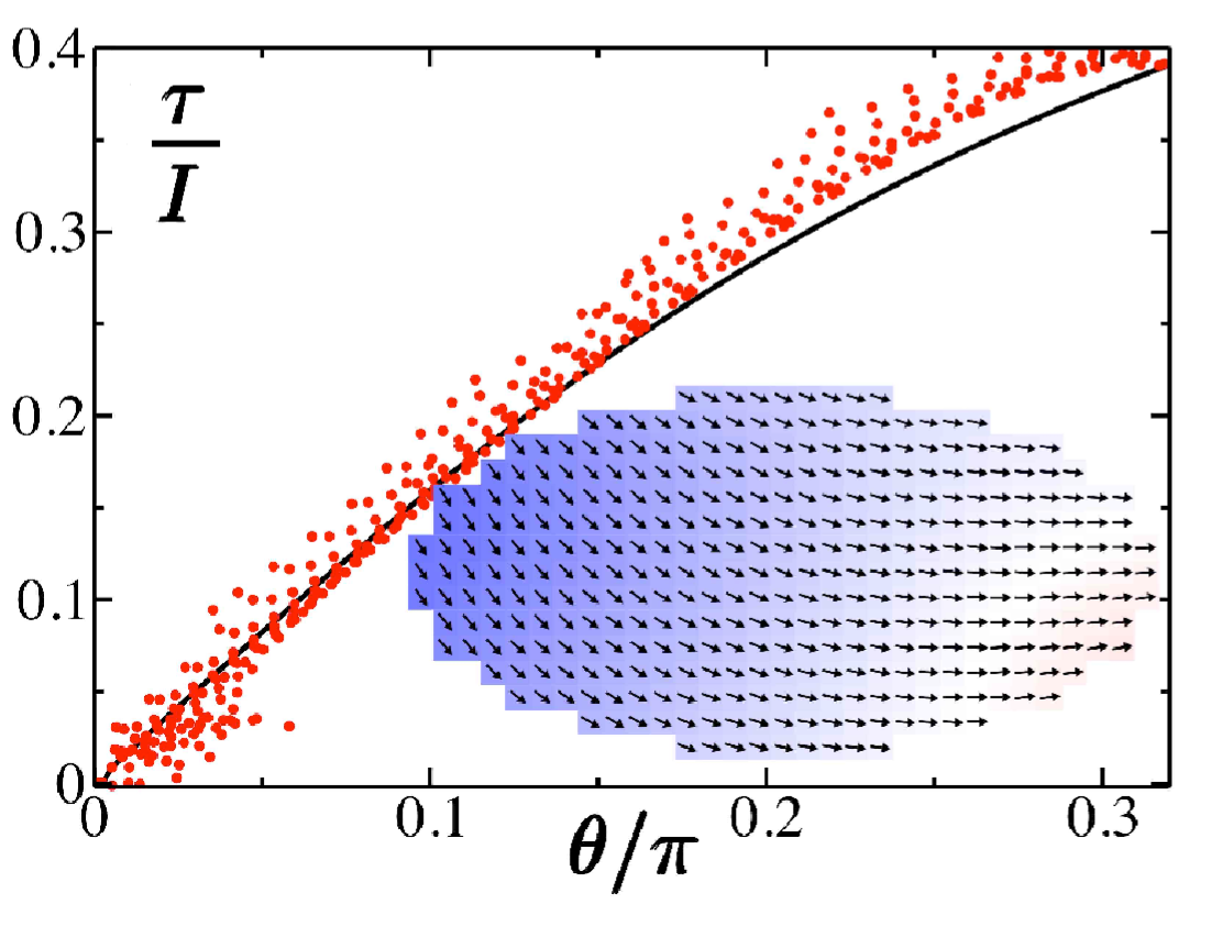
Figure 5: Torque $\tau$ per total current $I$ as a function of the local angle $\theta$ between the magnetization of the free layer and the reference magnetization of the thick layer for a ${\rm Cu_{48}|IrMn_{8}|Py_{8}|Cu_{4}|Py_{8}|Cu_{20}|Pt_{8}|Cu_{100}}$ pillar for a current density $I=2.5\,10^{7}A.cm^{-2}$. The full black line corresponds to 1D CRMT calculation while the cloud of red dots corresponds to the CRMT3D calculation. Inset: reference magnetic configuration of the free layer, calculated with micro-magnetic simulations Miltat and Donahue (2007).

To conclude this paper, we take advantage of the capability of CRMT3D to treat systems with magnetic texture and perform a study of spin transfer torque in a spin valve. We aim at evaluating the role of magnetic texture which is often disregarded in the calculation of spin torque made in micro-magnetic simulations. Our nanopillar corresponds to the following stack: ${\rm Cu_{48}|IrMn_{8}|Py_{8}|Cu_{4}|Py_{8}|Cu_{20}|Pt_{8}|Cu_{100}}$. It consists of a polarizing layer pinned by the ${\rm IrMn}$ antiferromagnetic layer and a free $8\,nm$ permalloy layer. This setup basically corresponds to the experiments reported in Ref. Krivorotov et al. (2007) and has been designed in such a way that the current induced magnetization reversal behaves in a coherent way (i.e. as close to a macrospin as possible) so that in this situation the role of magnetic texture is believed to be fairly small. Nevertheless, the Oersted field which is present at high current introduces a small ”banana shape” magnetic texture, as shown in the inset of Fig. 5. Our starting point is the corresponding stationary magnetic configuration of the free layer obtained from a micromagnetic simulation in presence of the Oesterd field Miltat and Donahue (2007). In a second step, we perform two different calculations of the spin torque: (I) a full CRMT3D calculation the local spin transfer torque $\tau_{I}(x,y)$ in presence of the Banana shape magnetic texture (the polarizing layer which is pinned by the ${\rm IrMn}$ layer is supposed to have no magnetic texture). (II) We take an approach which ignores the role of in plane spin currents: one assumes that current density is homogeneous across the nanopillar and parametrize the local spin transfer torque $\tau=f(\theta)$ as a function of the angle $\theta$ between the (local) magnetization and the reference fixed polarizing layer. When the system acquires some magnetic texture one uses $\tau_{II}(x,y)\equiv f(\theta(x,y))$. The parametrization $f(\theta)$ is obtained using the one dimensional version of CRMT. The effective 1D approach (II) is equivalent to the 3D approach (I) in the absence of magnetic texture and has become quite common in dynamical micromagnetic studies of current induced phenomena Slonczewski (2002); Manschot et al. (2004); Xiao et al. (2004, 2007); Ralph and Stiles (2008). The results are shown in Fig. 5 where the effective 1D CRMT approach $\tau=f(\theta)$ (line) is contrasted with the full 3D calculation where $\tau_{II}(x,y)$ is plotted as a function of $\theta(x,y)$ (red dots). The apparent ”noise” of the CRMT3D calculation reflects the fact that the torque is not a function of $\theta$ only but fully depends on the spatial position $(x,y)$. One can see that even though the general picture is captured by the effective one dimensional approach, a typical error of more than $10\%$ may be observed. We expect that upon performing an integration of the (highly nonlinear) 3D Landau-Lifshitz-Gilbert equation, such a systematic error will result in strong inaccuracy, even in the favorable situation considered here. We conclude that micromagnetic simulations of real predictive power, which are highly desirable for spintronic applications, require to treat magnetic and transport degrees of freedom on equal footing. In particular, a natural route would be to perform full CRMT3D calculations of the spin transport properties of the device ”on the fly” during the micromagnetic simulation.