Analysis of the temperature influence on Langmuir probe measurements on the basis of gyrofluid simulations

Abstract

The influence of the temperature and its fluctuations on the ion saturation current and the floating potential, which are typical quantities measured by Langmuir probes in the turbulent edge region of fusion plasmas, is analysed by global nonlinear gyrofluid simulations for two exemplary parameter regimes. The numerical simulation facilitates a direct access to densities, temperatures and the plasma potential at different radial positions around the separatrix. This allows a comparison between raw data and the calculated ion saturation current and floating potential within the simulation. Calculations of the fluctuation-induced radial particle flux and its statistical properties reveal significant differences to the actual values at all radial positions of the simulation domain, if the floating potential and the temperature averaged density inferred from the ion saturation current is used.

This is the preprint version of a manuscript submitted to Plasma Physics and Controlled Fusion.

I Introduction

In the edge and scrape-off layer regions of magnetically confined plasmas the fluctuating plasma density ${n=n_{\rm{e}}\simeq n_{\rm{i}}}$, the plasma potential $\Phi$ and the radial particle flux $\Gamma_{\rm{r}}$ are usually inferred from Langmuir probe measurements. However, the quantities measured by conventional cold Langmuir probes are the ion saturation current $I_{\rm{is}}$ and the floating potential $V_{\rm{fl}}$. Following the elementary Langmuir probe theory, these are related to the density and the plasma potential by expressions involving the electron and ion temperatures $T_{\rm{e}}$ and $T_{\rm{i}}$ (Schrittwieser2002 –Stangeby1990 ):

$$I_{\rm{is}} = A_{\rm{i}}en\sqrt{\frac{k_{\rm{B}}(T_{\rm{e}}+T_{\rm{i}})}{m_{\rm{i}}}}$$ (1)

$$V_{\rm{fl}} = \Phi-\left(\frac{k_{\rm{B}}T_{\rm{e}}}{e}\right)\ln\left(\frac{I_{\rm{es}}}{I_{\rm{is}}}\right)=\Phi-\left(\frac{k_{\rm{B}}T_{\rm{e}}}{e}\right)\ln\left(\frac{A_{\rm{e}}}{A_{\rm{i}}}\sqrt{\frac{T_{\rm{e}}}{T_{\rm{e}}+T_{\rm{i}}}}\sqrt{\frac{m_{\rm{i}}}{2\pi m_{\rm{e}}}}\right).$$ (2)

A Maxwellian electron velocity distribution is assumed, secondary electron emission from the probe is neglected and the electron saturation current $I_{\rm{es}}$ is given by $I_{\rm{es}}=A_{\rm{e}}en(1/4)\sqrt{(8k_{\rm{B}}T_{\rm{e}})/(\pi m_{\rm{e}})}$, using the random thermal current density. $A_{\rm{e}}$ and $A_{\rm{i}}$ specify the probe collecting areas for electrons and ions, respectively. Depending on the magnetic field strength, these areas can be differing for the two species, as stated in Schrittwieser2002 . At any rate, to determine density and plasma potential from the measured quantities, electron and ion temperatures have to be taken into account, although $T_{\rm{i}}$ is frequently assumed to be equal to $T_{\rm{e}}$. This is mainly due to the fact that in the edge region of fusion devices there is often no data available for the ion temperature.

The measurement of electron temperature fluctuations by means of classical Langmuir probes requires a sweeping of a preferably complete probe characteristic. This results in a lower time resolution of the respective time series compared to data acquired by floating or negatively biased $I_{\rm{is}}$ probe pins, although the method has undergone further development towards fast sweeping probes (Mueller2010 -Hidalgo1992 ). Alternatively, triple probes (Chen1965 , Xu2007 ) or the harmonics technique (Boedo1999 -Rudakov2001 ) can be used to measure fluctuations of $T_{\rm{e}}$. In addition, more sophisticated probes such as emissive probes (Schrittwieser2002 , Schrittwieser2008 ), in contrast to conventional cold probes, or ball-pen probes (Horacek2010 , Adamek2010 ) have been developed. These kind of probes are aimed at measuring the plasma potential directly and a combination of cold probes and ball-pen or emissive probes also allows a derivation of the electron temperature Adamek2002 . Nevertheless most probe measurements in the edge of large fusion devices are still based upon data measured by classical Langmuir probes. For estimations of the radial particle flux $\Gamma_{\rm{r}}=\tilde{n}\tilde{v_{\rm{r}}}$, the radial velocity is commonly calculated from gradients of the floating potential instead of the plasma potential Kirk2011 and the density is calculated from $I_{\rm{is}}$ using only average values for the temperatures.

The aim of this paper is to use numerical gyrofluid simulations to compare time series of density $n$, plasma potential $\Phi$ and temperatures $T_{\rm{e}}$, $T_{\rm{i}}$ with simulated values of ion saturation current $I_{\rm{is}}$ and floating potential $V_{\rm{fl}}$. The difference between the two corresponding datasets of $\Phi$ and $V_{\rm{fl}}$ is to some extent comparable to the difference between emissive and conventional probe measurements, although the potential measured by the former still deviates from the actual plasma potential by a certain, albeit smaller temperature-dependent factor Schrittwieser2008 .

For the simulations the nonlinear three-dimensional electromagnetic gyrofluid turbulence code GEMR has been used, which comprises a six-moment gyrofluid model for electrons and ions in a circular toroidal geometry and features energetic consistency (Scott2006 -Ribeiro2008 ). The coordinate system in use consists of a flux surface label ($x$) defining the radial position, a field line label within the flux surface ($y$) and a position along the field line ($s$) Scott2001 . For diagnostic purposes, the code delivers time series of fluctuating electron and ion densities, plasma potential, temperatures and parallel velocities, amongst others. Thus, the knowledge of these quantities including electron and ion temperatures allows the calculation of ion saturation current and floating potential. So the significance of temperature fluctuations with regard to density and potential measurements can be investigated. Moreover, the analysis can be performed at different simulated probe positions in the radial computation domain, which in our nominal case is $(r/a=1\pm 0.06)$, with $a$ being the minor radius.

Typical ASDEX Upgrade edge values have been chosen as input parameters for the simulation. The model can be regarded as global in the sense that there is a global variation of profiles, although the parameters are constant Scott2006 . Although no turbulence code can as yet self-consistently achieve an H–mode, magneto-hydrodynamic ideal ballooning modes (IBMs), which are commonly assumed to cause edge localised modes of type I, can be simulated by incorporating experimental H-mode density and temperature pedestal profiles n(r) and T(r) as initial state Kendl2010 . Ideal ballooning (ELM-like) blowouts in experiment and simulation are always connected with large fluctuations in density, temperature and plasma potential, so a comprehensive analysis of the temperature influence on floating potential and ion saturation current in this case is a reasonable addition to investigations of simulations in saturated L-mode state.

In the following sections the details of the comparison between plasma density and ion saturation current, plasma potential and floating potential and characteristics of the particle flux in L-mode situation (section 2) as well as IBM blowout situation (section 3) are presented. Possible reasons for the varying discrepancy between the actual quantities and the simulated Langmuir probe measurements are also addressed and the role of temperature fluctuations is discussed.

II Saturated L-mode situation

The first situation corresponds to an operation in saturated L-mode. That means, the electron dynamical plasma beta $\beta_{\rm{e}}=(\mu_{0}p_{\rm{e}})/B^{2}$ is chosen low enough not to be ideal ballooning unstable ($\beta_{\rm{e}}\approx 9.4\cdot 10^{-5}$) and electron and ion heat sources as well as density sources are set to a moderate level. The background mid-pedestal parameters for this case are $T_{\rm{e}}=150$ eV and $T_{\rm{i}}=180$ eV for the temperatures, $n_{\rm{e}}=n_{\rm{i}}=1.25\cdot 10^{19}$ m^-3 for the densities, $B=2.0$ T for the background magnetic field, $L_{\rm{T}}=L_{\perp}=3.0$ cm for the perpendicular temperature gradient length and $L_{\rm{n}}=6.0$ cm for the density gradient length. For the ion mass, the deuterium mass $m_{\rm{D}}=3670m_{\rm{e}}$ is used. Major torus radius and aspect ratio (major divided by minor radius) conform to ASDEX Upgrade values with $R=1.65$ m and $R/a=3.3$, while a circular flux-surface geometry is used.

The radial domain, whose direction is defined as the $x$-direction in the code, is divided into $n_{x}=64$ grid points. These are not equally spaced in terms of radius but in terms of volume, which for the present purpose makes a slight but not decisive difference. The $y$-direction is divided into $n_{y}=512$ grid points, the $s$-direction into $n_{s}=16$ grid points and the averaged grid size perpendicular to the magnetic field is $1.06\rho_{\rm{s}}\times 1.39\rho_{\rm{s}}$ (with $\rho_{\rm{s}}\approx 0.88$ mm). The analysed L-mode time series have a length of $11000$ data points and a temporal resolution of $0.0826\,\mathrm{\mu s}$ (total duration $0.908\,\mathrm{ms}$).

Especially in the outer scrape-off layer region of the radial domain ($x\sim 33-64$) the numerical (Arakawa)–scheme occasionally delivers unphysical negative density and temperature values in the presence of steep propagating gradients, arising from Gibbs oscillations. Therefore we added the absolute value of the largest negative value multiplied by an offset factor $\lambda_{\rm{os}}$ to all values of the time series at all positions, e.g. for the density, $n_{\rm{i},\mathit{x}}$ = $\bar{n}_{\rm{i},\mathit{x}}+\lambda_{\rm{os}}|\rm{Min}({\bar{n}_{\rm{i}}})|$, where $\bar{n}_{\rm{i},\mathit{x}}$ is the uncorrected time series at $x$ and the minimum of all values in the radial domain is used. As offset factor, $\lambda_{\rm{os}}=1.01$ has been chosen.

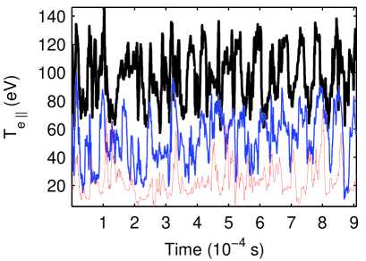
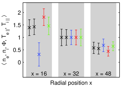
Figure 1: (a) Time series of the electron temperature $T_{\rm{e}\parallel}$. (b) Mean values and standard deviations of electron and ion density $n_{\rm{e}}$ and $n_{\rm{i}}$ (black), plasma potential $\Phi$ (blue), electron temperature $T_{\rm{e}\parallel}$ (red) and ion temperature $T_{\rm{i}\parallel}$ (green), normalised to the respective mean at $x=32$, for the L-mode case at different radial positions. The simulation grid point $x=16$ (black bold line in (a)) corresponds to the radial distance of $\sim-14.8$ mm $\approx-16.7\rho_{\rm{s}}$, $x=32$ (blue line in (a)) to $\sim 0.4$ mm $\approx 0.5\rho_{\rm{s}}$ and $x=48$ (red thin line in (a)) to $\sim 15.2$ mm $\approx 17.2\rho_{\rm{s}}$, measured from the separatrix

The simulation run exhibits an ion temperature gradient (ITG) driven interchange overshoot quite at the beginning and then saturates rather quickly to an L-mode-like state. For the analysis and the plots presented in this section only the well saturated part after the initial transient has been taken into account. Fig. 1 exemplary shows the time series of $T_{\rm{e}\parallel}$ as well as mean values and standard deviations of $n_{\rm{e}}$ and $n_{\rm{i}}$, $\Phi$, $T_{\rm{e}\parallel}$ and $T_{\rm{i}\parallel}$ at different radial positions (inside, near and outside the separatrix).

Both here and in the following parts of the L-mode section, plots showing the temporal evolution of a quantity are based on data taken near the outboard midplane, whereas plots of time averaged data are composed from the individual results of different toroidal positions to provide better statistics. The radial position outside the separatrix ($\sim 1.5$ cm, red thin lines) corresponds approximately to the region of Langmuir probe measurements in ASDEX Upgrade, which are typically positioned few centimeters outside the last closed flux surface. A separate treatment of parallel and perpendicular temperatures ($T_{\rm{e}\parallel}$, $T_{\rm{i}\parallel}$ and $T_{\rm{e}\perp}$, $T_{\rm{i}\perp}$) arises from the construction of moments in the gyrofluid equations Beer1996 . However, in the present case there is no major difference between both components and only time series of the parallel temperatures have been used to calculate the quantities of the synthetic probe.

II.1 Plasma density vs. ion saturation current

The ion saturation current $I_{\rm{is}}$ has been calculated from ion density and the temperatures of electrons and ions according to eq. 1 (with $A_{\rm{e}}=A_{\rm{i}}$ defining the cross section of the probe). As the characteristics of the $n_{\rm{i}}$, $T_{\rm{e}\parallel}$ and $T_{\rm{i}\parallel}$ time series are rather similar, there are no striking differences between the ion saturation current, which is essentially a product between them, with the sum of temperatures appearing as a square root, and the underlying quantities and it still shows a qualitatively comparable temporal evolution.

For evaluations of the radial particle flux from experimentally measured probe data it is necessary to know, amongst others, the particle density. Although the conversion can easily be done using eq. 1, in many experimental cases only average temperature values are available (e. g. evaluated by sweeping the Langmuir probe). Hence it makes sense to recalculate $n_{\rm{i}}$ from $I_{\rm{is}}$ using averaged values of the simulated $T_{\rm{e}\parallel}$ and $T_{\rm{i}\parallel}$ time series for each $x$-position in the radial domain and to compare the results with the precise $n_{\rm{i}}$ time series. Both signals are plotted in fig. 2 for a position within the SOL. Inside and near the separatrix similar results have been obtained. The difference between $n_{\rm{i}}^{\rm{avg}}$ and $n_{\rm{i}}$, given by

$$n_{\rm{i}}^{\rm{avg}}-n_{\rm{i}}=\frac{I_{\rm{is}}\sqrt{m_{\rm{i}}}}{A_{\rm{i}}e}\left(\frac{1}{\sqrt{k_{\rm{B}}(T_{\rm{e}}^{\rm{avg}}+T_{\rm{i}}^{\rm{avg}})}}-\frac{1}{\sqrt{k_{\rm{B}}(T_{\rm{e}}+T_{\rm{i}})}}\right),$$ (3)

is particularly large at points of maxima and minima, but rather small elsewhere. As $n_{\rm{i}}^{\rm{avg}}=n_{\rm{i}}\sqrt{(T_{\rm{e}}+T_{\rm{i}})/(T_{\rm{e}}^{\rm{avg}}+T_{\rm{i}}^{\rm{avg}})}$, the ratio of the actual temperature values to their average values is the decisive factor. The average temperatures are smaller than the maxima, which results in larger values of $n_{\rm{i}}^{\rm{avg}}$ at these positions (the temperatures appear in the denominator in eq. 3). For the minima, the same statement holds vice versa.

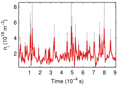
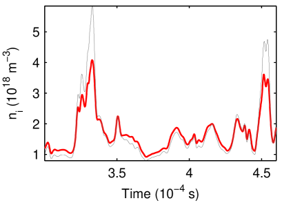
Figure 2: (a) L-Mode time series of code output $n_{\rm{i}}$ (red bold line) and $n_{\rm{i}}^{\rm{avg}}$ (black thin line) calculated from $I_{\rm{is}}$ using averaged values for $T_{\rm{e}\parallel}$ and $T_{\rm{i}\parallel}$. The data is plotted for a radial position $\sim 15.2$ mm $\approx 17.2\rho_{\rm{s}}$ outside the separatrix. (b) Detailed evolution of a $160\,\mathrm{\mu s}$ time frame

II.2 Plasma potential vs. floating potential

Fig. 3 shows a comparison of the plasma potential $\Phi$ and the floating potential $V_{\rm{fl}}$ for a position within SOL, computed by means of eq. 2. A clear difference is evident, as is to be expected, both in mean values and fluctuations. Comparing different radial positions, the mean offset between $\Phi$ and $V_{\rm{fl}}$ is decreasing from the inside to the outside. In terms of mathematics, the difference is caused by a product of the electron temperature in energy units, divided by $e$, and a dimensionless quantity, which depends on the temperature as well:

$$\Delta^{\rm{real}}=\left(\frac{k_{\rm{B}}T_{\rm{e}}}{e}\right)\ln\left(\frac{A_{\rm{e}}}{A_{\rm{i}}}\sqrt{\frac{T_{\rm{e}}}{T_{\rm{e}}+T_{\rm{i}}}}\sqrt{\frac{m_{\rm{i}}}{2\pi m_{\rm{e}}}}\right)=\left(\frac{k_{\rm{B}}T_{\rm{e}}}{e}\right)\Delta.$$ (4)

If the temperature is assumed to be constant, i.e. all temperature fluctuations are neglected, the latter can be understood as average difference $\Delta^{\rm{avg}}$ between $\Phi$ and $V_{\rm{fl}}$ (also referred to as $\alpha$), normalised by $e/(k_{\rm{B}}T_{\rm{e}})$ (see Schrittwieser2002 ). It can roughly be estimated for our nominal case with $T_{\rm{i}}=1.2T_{\rm{e}}$ and $A_{\rm{i}}=A_{\rm{e}}$ to be $\Delta^{\rm{avg}}\approx 2.79$. Thus on average the normalised difference for a certain relation of $T_{\rm{e}}$ and $T_{\rm{i}}$ is constant and deviations are mainly due to temperature fluctuations. On the other hand, the background mid-pedestal temperature values used here are only reference values. For all radial positions, but especially within the scrape-off layer the simulated temperature relation can differ considerably from this. Consequently, $\Delta^{\rm{avg}}$ is subject to radial variations (see fig. 5). Taking into account that the temperature is not constant results in a fluctuating time series $\Delta$, which is plotted for one exemplary position within the SOL in fig. 4. The radial profile of its standard deviation is shown as light grey area in fig. 5. In the same figure, source and sink regions of the GEMR simulation model are indicated by dark grey shadings. The radial positions affected by these mechanisms are removed in all subsequent profile plots, as they should be excluded from the interpretation.

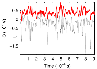
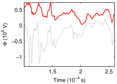
Figure 3: (a) L-Mode time series of $\Phi$ (red bold line) and $V_{\rm{fl}}$ (black thin line) for a radial position $\sim 15.2$ mm $\approx 17.2\rho_{\rm{s}}$ outside the separatrix. (b) Detailed evolution of a $160\,\mathrm{\mu s}$ time frame

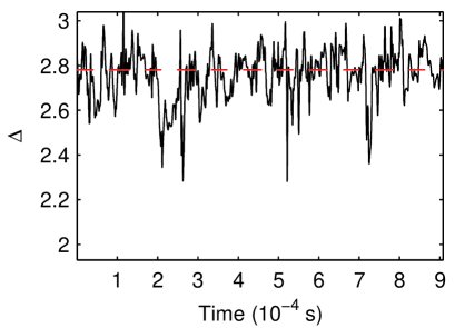
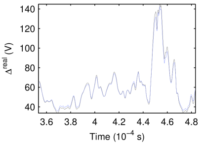
Figure 4: (a) Normalised difference $\Delta$ between floating and plasma potential for a position $\sim 15.2$ mm $\approx 17.2\rho_{\rm{s}}$ outside the separatrix, calculated from the fluctuating temperature time series (black solid line) and from constant temperature values averaged at the corresponding radial position (red dashed line). (b) Detailed evolution $130\,\mathrm{\mu s}$ of the actual difference $\Delta^{\rm{real}}$ between floating and plasma potential (black line) and $((k_{\rm{B}}T_{\rm{e}})/{e})\Delta^{\rm{avg}}$ (blue line) within the SOL

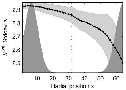
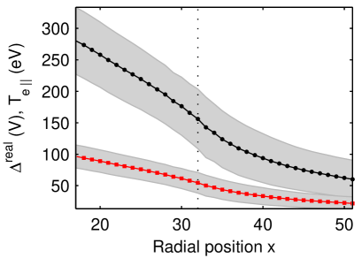
Figure 5: (a) Radial profile of $\Delta^{\rm{avg}}$ (black line with circles), standard deviation of exact $\Delta$ time series (light grey area) and source/sink regions of the GEMR simulation model (dark grey shading). (b) Radial profile of $\langle\Delta^{\rm{real}}\rangle$ (black line with circles), $\langle T_{\rm{e}}\rangle$ (red line with squares) and the respective standard deviations (light grey area). The location of the separatrix is indicated by the dotted line

It is important to note, that $\Delta$ is the normalised difference between $\Phi$ and $V_{\rm{fl}}$. It can be a useful quantity for rough evaluations, if only average temperatures are available. A quantitative estimation of the actual difference requires the calculation of $\Delta$ multiplied by $(k_{\rm{B}}T_{\rm{e}})/e$ (eq. 4) for every time step and for all positions. Thus the shape and phase of the temperature time series, which is varying depending on the measurement position, has a direct influence on the difference between plasma and floating potential.

As the mean temperature $\langle T_{\rm{e}}\rangle$ strongly decreases within the radial simulation domain, the actual difference $\Delta^{\rm{real}}$ ($\propto T_{\rm{e}}\Delta$) between floating and plasma potential is larger inside the separatrix and becomes smaller in the SOL (fig. 5). The difference in terms of fluctuation amplitudes seems to be somewhat larger inside and near the separatrix, which is due to large temperature fluctuations in this region, but a significant distinction of the general shape is evident at all radial positions.

In order to emphasise the role of the electron temperature fluctuations, a comparison between the temporal evolution of $\Delta^{\rm{real}}=((k_{\rm{B}}T_{\rm{e}})/{e})\Delta$ and the quantity $((k_{\rm{B}}T_{\rm{e}})/{e})\Delta^{\rm{avg}}$ is shown in fig. 4. There are only faint differences visible, indicating the predominance of the fluctuations of $T_{\rm{e}}$ compared to the fluctuations of $\Delta$ and, consequently, to the fluctuations of $T_{\rm{i}}$. This behaviour can be observed in the entire radial domain, with a slightly decreasing difference between the two terms plotted in fig. 4 from the inside to the outside and therefore a decreasing importance of a precise $\Delta$.

As stated in ref. Adamek2002 , the differences in fluctuations of $V_{\rm{fl}}$ and $\Phi$ are determined not only by fluctuations of the electron temperature, but also by the phase relation between temperature and potential. This becomes evident from the difference of the corresponding root mean square values,

$$[\rm{RMS}(\tilde{V}_{\rm{fl}})]^{2}-[\rm{RMS}(\tilde{\Phi})]^{2}=[\rm{RMS}(\tilde{\Delta}^{\rm{real}})]^{2}-2\langle\tilde{\Phi}\tilde{\Delta}^{\rm{real}}\rangle.$$ (5)

The tilde indicates fluctuating parts and the RMS of, for example, $\tilde{\Phi}$ is given by $\langle\tilde{\Phi}^{2}\rangle^{1/2}$, which in the case of fluctuations with zero mean reflects the standard deviation (except for a slightly different normalisation). Fig. 6 shows radial profiles of the left-hand side of eq. 5 and the two terms on the right-hand side. It is apparent, that although the contribution of $\tilde{\Delta}^{\rm{real}}$ ($\propto\tilde{T}_{\rm{e}}$) is clearly dominant, the influence of the cross phase between $\tilde{\Phi}$ and $\tilde{\Delta}^{\rm{real}}$, represented by $\langle\tilde{\Phi}\tilde{\Delta}^{\rm{real}}\rangle$, is of non-negligible magnitude and radially varying, with largest absolute values near the separatrix and within the SOL, but rather small values inside the separatrix. A comprehensive analysis of the phase relation between temperature and potential at different radial positions by means of time-resolved Wavelet methods is currently in progress and will be presented in a future work.

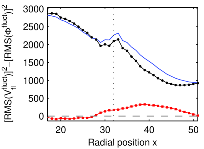
Figure 6: (a) Radial profile of $[\rm{RMS}(\tilde{V}_{\rm{fl}})]^{2}-[\rm{RMS}(\tilde{\Phi})]^{2}$ (black line with circles), which is equal to the difference of $[\rm{RMS}(\tilde{\Delta}^{\rm{real}})]^{2}$ (blue solid line) and $2\langle\tilde{\Phi}\tilde{\Delta}^{\rm{real}}\rangle$ (red line with squares) The tilde indicates fluctuating parts and RMS root mean square values

The present calculation of the floating potential using simulated temperature time series depends to a certain degree on the artificial offset factor $\lambda_{\rm{os}}$, which has a decisive influence on the temperature averages and therefore also on the mean offset between $\Phi$ and $V_{\rm{fl}}$. Apart from that, time series of $\Delta$ are affected, as the logarithm in the conversion equation eq. 2 reacts quite sensitive on variations of the temperature minima, whose difference to zero is defined by $\lambda_{\rm{os}}$. As a consequence, not only the distinct negative peaks in fig. 4, but also the radial profiles of $\Delta^{\rm{avg}}$ and $\rm{Stddev}(\Delta)$ change their characteristics depending on the chosen offset factor. Since $\lambda_{\rm{os}}$ has no effect on temperature fluctuations, its impact on the fluctuating part and the standard deviation of $\Delta^{\rm{real}}$ and on the comparison in fig. 4 is weak. That implies, that although the shape of the $\Delta$ time series and the mean offset between $\Phi$ and $V_{\rm{fl}}$ is affected by this numerical issue and the artificial offset, the influence of electron and ion temperature fluctuations on calculations of the floating potential can nevertheless be studied. This applies even more to calculations of the radial particle flux, because only potential gradients are of importance there. A prerequisite for any considerations about the influence of small fluctuations on potential measurements is the question, whether an experimental probe is in principle able to react almost instantaneously to temperature fluctuations. This can indeed be assumed, because density fluctuations, which have similar characteristics and a comparable ratio of fluctuations to mean, can be detected.

II.3 Radial particle flux

One of the most important quantities for the statistical analysis of experimental measurements is the turbulent fluctuation-induced averaged radial particle flux (Carreras1996 –Endler1995 and Schrittwieser2008 ), defined by

$$\Gamma_{\rm{r}}=\langle\tilde{n}\tilde{v_{\rm{r}}}\rangle\approx\frac{\langle\tilde{n}\tilde{E}_{\rm{pol}}\rangle}{B},$$ (6)

where the fluctuating radial drift velocity is assumed to be the radial component of the fluctuating $\mathbf{\tilde{E}}\times\mathbf{B}$ velocity, $\tilde{v}_{\rm{r}}\approx v_{\mathbf{\tilde{E}}\times\mathbf{B}}=\tilde{E}_{\rm{pol}}/B$. Appropriate averaging is indicated by $\langle\cdot\rangle$. The poloidal electric field can be approximated by taking the difference between two potential measurements divided by their poloidal separation distance. In our simulations, this distance is given by $d_{12}\approx 2.5\,\mathrm{mm}$. Replacing the density by the expression for the ion saturation current $I_{\rm{is}}$ from eq. 1 yields

$$\Gamma_{\rm{r}}\approx\frac{1}{B}\left\langle\left(\frac{1}{A_{\rm{i}}e}\sqrt{\frac{m_{\rm{i}}}{k_{\rm{B}}(T_{\rm{e}}+T_{\rm{i}})}}I_{\rm{is}}\right)\left(\frac{V_{\rm{fl},1}-V_{\rm{fl},2}}{d_{12}}\right)\right\rangle.$$ (7)

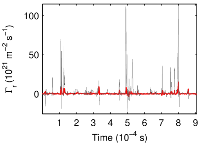
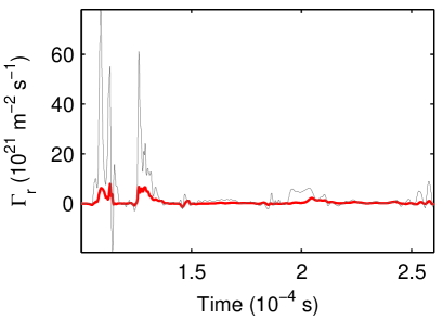
Figure 7: Radial particle flux $\Gamma_{\rm{r}}$ calculated from plasma potential and density ($\Gamma_{\rm{r}}^{\rm{real}}$, red bold line) and from floating potential and ion saturation current ($\Gamma_{\rm{r}}^{\rm{m}}$, black thin line). The data is plotted for a radial position $\sim 15.2$ mm $\approx 17.2\rho_{\rm{s}}$ outside the separatrix. (b) Detailed evolution of a $160\,\mathrm{\mu s}$ time frame.

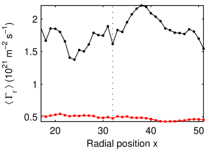
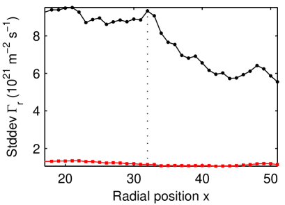
Figure 8: (a) Radial profiles of the time averaged particle flux $\langle\Gamma_{\rm{r}}\rangle$ (averaged across the entire simulation time), (b) standard deviation $\rm{Stddev}(\Gamma_{\rm{r}})$. Real values are plotted as red line with squares, measured values as black line with circles

Both, the synthetically measured particle flux $\Gamma_{\rm{r}}^{\rm{m}}$ (using $V_{\rm{fl}}$ and densities inferred from $I_{\rm{is}}$ and averaged temperatures) and the real particle flux $\Gamma_{\rm{r}}^{\rm{real}}$ (using code outputs $\Phi$ and $n_{\rm{e}}$) have been calculated and their temporal evolution, representing the instantaneous particle flux, is plotted in fig. 7. The time series of $\Gamma_{\rm{r}}^{\rm{m}}$ exhibit much larger fluctuations than that of $\Gamma_{\rm{r}}^{\rm{real}}$ at all radial positions, but especially inside and near the separatrix, which is clearly visible in the radial profile of the standard deviation of the time-averaged flux (fig. 8). On average, $\rm{Stddev}(\Gamma_{\rm{r}}^{\rm{m}})$ is $\sim 7$ times larger than $\rm{Stddev}(\Gamma_{\rm{r}}^{\rm{real}})$. Magnitudes and radial profiles of the mean fluxes $\langle\Gamma_{\rm{r}}^{\rm{real}}\rangle$ and $\langle\Gamma_{\rm{r}}^{\rm{m}}\rangle$ depend on the length of the investigated time range, but significant differences can be observed in any case (fig. 8, $\langle\Gamma_{\rm{r}}^{\rm{m}}\rangle\sim 3.5$ times larger than $\langle\Gamma_{\rm{r}}^{\rm{real}}\rangle$). The use of an averaged temperature value in the density calculation only gives rise to small deviations (see fig. 2) and is not responsible for the large discrepancy in terms of fluctuations. Hence it must primarily be due to the radial velocity calculated from the gradient of the floating potential.

The equivalent use of the floating potential instead of the plasma potential, which is the usual procedure to estimate the particle flux from Langmuir probe measurements, is based on the assumption, that the difference between plasma and floating potential is roughly constant at two closely spaced locations. As only the difference between two adjacent time series is relevant, the error caused by using $V_{\rm{fl}}$ instead of $\Phi$ is expected to be small, depending on different deviations from this constant at the two locations. Such deviations have been discussed in the previous section, but for radially varying positions, whereas here different positions in the $y$-direction of the simulation model are of importance. Fluctuations of time series at these positions correspond to fluctuations of two poloidally separated positions, because $k_{\parallel}\ll k_{\perp}$. For $V_{\rm{fl}}=\Phi-[(k_{\rm{B}}T_{\rm{e}})/e]\Delta$, the difference between approximations of plasma potential gradient and floating potential gradient is given by

$$\frac{\Phi_{1}-\Phi_{2}}{d_{12}}-\frac{V_{\rm{fl},1}-V_{\rm{fl},2}}{d_{12}} = \frac{1}{d_{12}}\left[\Phi_{1}-\Phi_{2}-\left(\Phi_{1}-\frac{k_{\rm{B}}T_{\rm{e},1}}{e}\Delta_{1}\right)+\left(\Phi_{2}-\frac{k_{\rm{B}}T_{\rm{e},2}}{e}\Delta_{2}\right)\right]$$ (8)

$$= \frac{1}{d_{12}}\frac{k_{\rm{B}}}{e}\left(T_{\rm{e},1}\Delta_{1}-T_{\rm{e},2}\Delta_{2}\right).$$

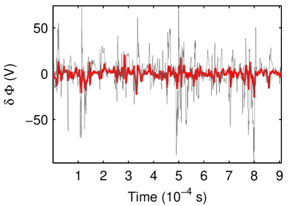
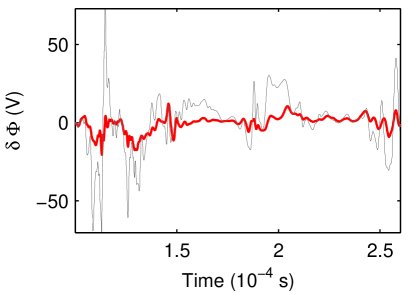
Figure 9: (a) Difference between two time series $\Phi_{1}$ and $\Phi_{2}$ (red bold line) and between $V_{\rm{fl},1}$ and $V_{\rm{fl},2}$ (black thin line), collected at the poloidally adjacent positions used for the estimation of $\tilde{v_{\rm{r}}}$. The data is plotted for a radial position $\sim 15.2$ mm $\approx 17.2\rho_{\rm{s}}$ outside the separatrix. (b) Detailed evolution of a $160\,\mathrm{\mu s}$ time frame.

This expression vanishes, if $T_{\rm{e},1}=T_{\rm{e},2}$ and $\Delta_{1}=\Delta_{2}$ is assumed for the two adjacent positions. According to fig. 9, which shows $\delta\Phi=\Phi_{1}-\Phi_{2}$ and $\delta V_{\rm{fl}}=V_{\rm{fl},1}-V_{\rm{fl},2}$, this is clearly not the case, so there must be a significant difference between these quantities. The second part of equation eq. 8 can be further expanded by splitting the respective quantities into mean values and fluctuations:

$$\left(T_{\rm{e},1}\Delta_{1}-T_{\rm{e},2}\Delta_{2}\right)= \Big{[}\big{(}\langle T_{\rm{e},1}\rangle\langle\Delta_{1}\rangle-\langle T_{\rm{e},2}\rangle\langle\Delta_{2}\rangle\big{)}+\big{(}\langle T_{\rm{e},1}\rangle\tilde{\Delta}_{1}-\langle T_{\rm{e},2}\rangle\tilde{\Delta}_{2}\big{)}$$ (9)

$$+\big{(}\langle\Delta_{1}\rangle\tilde{T}_{\rm{e},1}-\langle\Delta_{2}\rangle\tilde{T}_{\rm{e},2}\big{)}+\big{(}\tilde{T}_{\rm{e},1}\tilde{\Delta}_{1}-\tilde{T}_{\rm{e},2}\tilde{\Delta}_{2}\big{)}\Big{]}.$$

A small offset between the two time series of $\delta\Phi$ and $\delta V_{\rm{fl}}$ is caused by slightly different mean values of $T_{\rm{e},1}$ and $T_{\rm{e},2}$ as well as $\Delta_{1}$ and $\Delta_{2}$ (fig. 10), which is expressed by the first term on the right-hand side of eq. 9. The remaining terms, the second last of which providing by far the largest contribution, are related to the strong fluctuations of $\delta V_{\rm{fl}}$. These originate from differences in the fluctuating parts of $T_{\rm{e},1}$ and $T_{\rm{e},2}$ (fig. 10) and, accordingly but of less importance, $\Delta_{1}$ and $\Delta_{2}$.

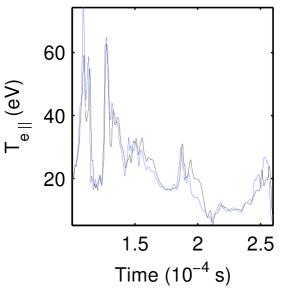
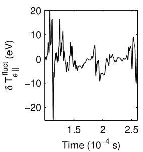
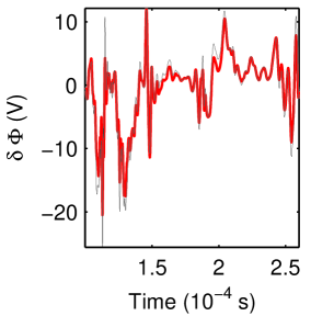
Figure 10: (a) Temperature time series $T_{\rm{e},1}$ (black line) and $T_{\rm{e},1}$ (blue line), collected at the two poloidally adjacent positions. (b) Difference between the fluctuating parts of the two temperature time series. (c) Difference between the two spatially adjacent time series for $\Phi$ (red bold line) and $V_{\rm{fl}}$ (black thin line) for the artificial case of small differences of the fluctuating temperature time series (see text). All plots show the detailed evolution of a $160\,\mathrm{\mu s}$ time frame for a radial position $\sim 15.2$ mm $\approx 17.2\rho_{\rm{s}}$ outside the separatrix

To point this out, $V_{\rm{fl}}$ and the differences $\delta\Phi$ and $\delta V_{\rm{fl}}$ of spatial adjacent time series have been calculated for the artificial case of temperature time series, which have equal mean and therefore no offset at the two positions, and whose difference in fluctuations is the same as before (fig. 10), but with much smaller amplitude ($1/10$). The result is plotted in fig. 10, where $\delta V_{\rm{fl}}$ is in substantial better agreement with $\delta\Phi$ than in fig. 9.

In order to investigate the impact of temperature fluctuations on statistical properties, probability distribution functions (PDF) have been computed. As shown in fig. 11 and fig. 12, there is a different behaviour inside and outside the SOL. Inside and near the separatrix, the PDF of the real particle flux features a larger skewness at most radial positions, whereas the kurtosis is largely of about the same magnitude. In the scrape-off layer, from a radial position of $\sim 6\,\mathrm{mm}\approx 6.8\rho_{\rm{s}}$ outside the separatrix, both the skewness and the kurtosis of $\Gamma_{\rm{r}}^{\rm{real}}$ are smaller than that of $\Gamma_{\rm{r}}^{\rm{m}}$, which indicates, that in the time series of $\Gamma_{\rm{r}}^{\rm{m}}$ strong deviations from the mean value occur even more frequently than in $\Gamma_{\rm{r}}^{\rm{real}}$.

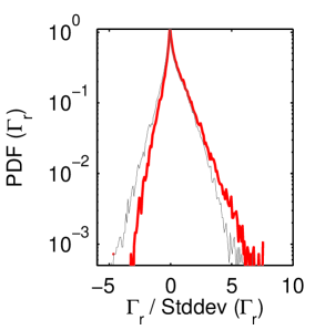
(a) Inside separatrix

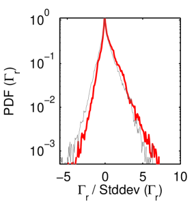
(b) Near separatrix

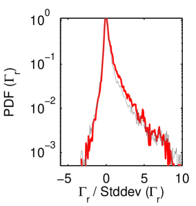
(c) Outside separatrix

Figure 11: PDF of the radial particle flux $\Gamma_{\rm{r}}$, calculated from plasma potential and density (red bold line) and from floating potential and ion saturation current (black thin line). The data is plotted at the radial positions (a) inside, (b) near and (c) outside the separatrix as specified in fig. 1

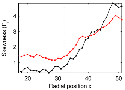
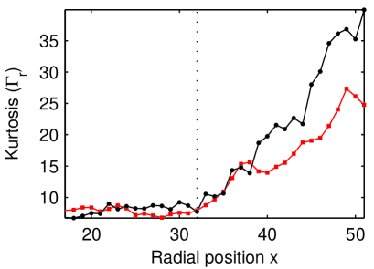
Figure 12: Radial profiles of (a) the Skewness and (b) the Kurtosis of real (red line with squares) and measured particle flux $\Gamma_{\rm{r}}$ (black line with circles)

Above investigations show, that both flux time series and their statistics are differing to a significant degree depending on whether temperature fluctuations are taken into account for the calculations. This seems to be the case not only for measurement positions inside and near the separatrix, but also within the SOL, where Langmuir probe measurements are typically located. Although the quantitative results of our numerical simulation might differ from the experimental situation in a fusion device and should not be taken as a reference, the importance of the fluctuating electron temperature is nevertheless evident. It should be mentioned, that variations of the offset factor $\lambda_{\rm{os}}$, which is used to compensate numerical errors of the simulated time series, only have small influence on this and do not change the overall flux features.

III Ideal ballooning mode blowout

As a next step, a simulated ELM type-I like ideal ballooning mode (IBM) situation has been analysed, which exhibits a large interchange blowout. A sudden burst connected with enhanced fluctuations is clearly visible in the time series of $T_{\rm{e}\parallel}$, which is shown as an example in fig. 13, but of course also in the signals of $n_{\rm{e}}$ and $n_{\rm{i}}$, $\Phi$, and $T_{\rm{i}\parallel}$. In the aftermath of the blowout the standard deviations of the temperatures and densities are lower compared to the L-mode case at most radial positions, but the standard deviations of the potential time series are larger (fig. 13). The background temperature and density parameters are $T_{\rm{e}}=300\,\mathrm{eV}$, $T_{\rm{i}}=360\,\mathrm{eV}$ and $n_{\rm{e}}=n_{\rm{i}}=2.5\cdot 10^{19}$ m^-3. Gradient lengths and background magnetic field remain unchanged compared to the L-mode case of the previous section. This yields $\beta_{\rm{e}}\approx 4.0\cdot 10^{-4}$ and allows the occurrence of an IBM instability, according to the MHD ideal ballooning criterion $\alpha_{\rm{m}}=q^{2}R\nabla\beta>\hat{s}$ (with $\beta=2\beta_{\rm{e}}$, safety factor $q=1.5+3.5(r/a)^{2}$ and magnetic shear parameter $\hat{s}=(r/q)(\partial q/\partial r)\rightarrow\hat{s}_{a}=1.4$ at the separatrix). Heat and density sources are set to a small value, in order to provide an IBM blowout as pure as possible and to prevent distortions caused by other effects. The averaged grid size perpendicular to the magnetic field is $0.75\rho_{\rm{s}}\times 0.98\rho_{\rm{s}}$ (with $\rho_{\rm{s}}\approx 1.25$ mm). The analysed IBM time series have a length of $15000$ data points and a temporal resolution of $\sim 0.0167\,\mathrm{\mu s}$ (total duration $0.25\,\mathrm{ms}$). All signals of this section are acquired near the outboard midplane. Further details on IBM simulations with GEMR can be found in ref. Kendl2010 .

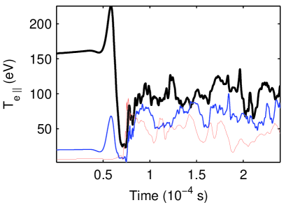
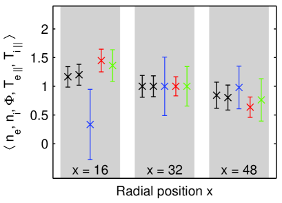
Figure 13: (a) Time series of the electron temperature $T_{\rm{e}\parallel}$. (b) Mean values and standard deviations of electron and ion density $n_{\rm{e}}$ and $n_{\rm{i}}$ (black), plasma potential $\Phi$ (blue), electron temperature $T_{\rm{e}\parallel}$ (red) and ion temperature $T_{\rm{i}\parallel}$ (green), normalised to the respective mean at $x=32$, in the aftermath of an IBM blowout at different radial positions. The simulation grid point $x=16$ (black bold line in (a)) corresponds to the radial distance of $\sim-14.8$ mm $\approx-11.8\rho_{\rm{s}}$, $x=32$ (blue line in (a)) to $\sim 0.4$ mm $\approx 0.34\rho_{\rm{s}}$ and $x=48$ (red thin line in (a)) to $\sim 15.2$ mm $\approx 12.2\rho_{\rm{s}}$, measured from the separatrix

III.1 Plasma density vs. ion saturation current and plasma potential vs. floating potential

Just as in the L-Mode case discussed above, there are no major differences between the time series of density and ion saturation current and both feature similar characteristics. If the density is inferred from $I_{\rm{is}}$ by means of averaged temperature values (fig. 14), the main features are preserved, apart from the time-dependent offset mentioned in subsection II.1, which results from averaging. As the use of time-averaged values is more defective for large density and temperature variations, it is most pronounced during the blowout.

$\Phi$, $V_{\rm{fl}}$ and $\Delta^{\rm{real}}$, the actual difference between plasma and floating potential, have also been calculated for the IBM case (fig. 14 and fig. 15). An individual investigation of $\Delta$ has been omitted, since according to section II.2 the inclusion of the factor $T_{\rm{e}}$ plays an important role. The predominance of $\tilde{T}_{\rm{e}}$ compared to $\tilde{\Delta}$ is still present, as a comparison between $\Delta^{\rm{real}}$ and $((k_{\rm{B}}T_{\rm{e}})/{e})\Delta^{\rm{avg}}$, shown in fig. 4 for the L-mode situation, yields similar results for IBM time series. Differences between fluctuations of $\Phi$ and $V_{\rm{fl}}$ are clearly noticeable at all radial positions, but due to the limited lengths of the IBM time series no reliable results for the standard deviation could be obtained, in particular before and during the blowout. After the blowout, the profile of the standard deviation seems to be similar to the L-mode case. Inside the separatrix, the IBM blowout leads to a strong reduction of the temperature, whereas near and beyond the separatrix it is increased. This is reflected in the temporal evolution of $\Delta^{\rm{real}}$. Fig. 15 shows radial profiles of $\langle\Delta^{\rm{real}}\rangle$ and $\langle T_{\rm{e}}\rangle$, separately averaged across the time range immediately before and after the blowout. Inside the separatrix the time average of the actual difference and the temperature is considerably larger before the blowout than afterwards. From a point near but not across the separatrix it is just the other way around. The decrease or increase of $\Delta^{\rm{real}}$ after the blowout has implications if the plasma potential is calculated from $V_{\rm{fl}}$ using temperatures averaged across the entire time domain, as the resulting time series will be either underestimated before the blowout and overestimated afterwards or vice-versa.

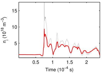
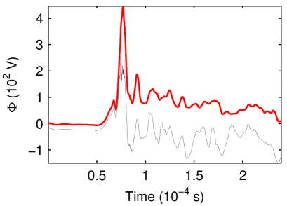
Figure 14: (a) IBM time series of code output $n_{\rm{i}}$ (red bold line) and $n_{\rm{i}}^{\rm{avg}}$ (black thin line) calculated from $I_{\rm{is}}$ using averaged values for $T_{\rm{e}\parallel}$ and $T_{\rm{i}\parallel}$. (b) IBM time series of $\Phi$ (red bold line) and $V_{\rm{fl}}$ (black thin line). The data is plotted for a radial position $\sim 15.2$ mm $\approx 12.2\rho_{\rm{s}}$ outside the separatrix.

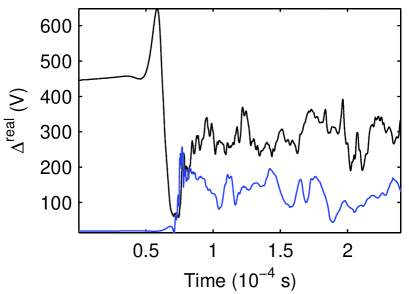
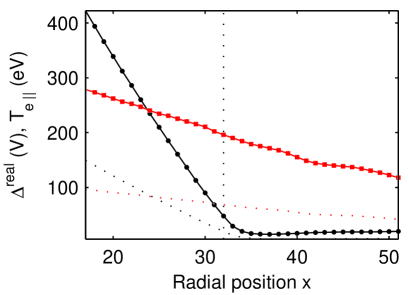
Figure 15: (a) Actual difference $\Delta^{\rm{real}}$ between floating and plasma potential for the radial positions $\sim 14.8$ mm $\approx 11.8\rho_{\rm{s}}$ inside (black line) and $\sim 15.2$ mm $\approx 12.2\rho_{\rm{s}}$ outside the separatrix (blue line). (b) Radial profile of $\langle\Delta^{\rm{real}}\rangle$ before (black line with circles) and after the blowout (red line with squares). Profiles of $\langle T_{\rm{e}}\rangle$ are plotted as dotted line.

III.2 Radial particle flux

Also in the IBM case, the instantaneous ”measured” radial particle flux $\Gamma_{\rm{r}}^{\rm{m}}$ calculated from $I_{\rm{is}}$ and $V_{\rm{fl}}$ shows much larger fluctuations than the real flux $\Gamma_{\rm{r}}^{\rm{real}}$. This is again primarily due to the use of $V_{\rm{fl}}$ instead of $\Phi$. The averaged temperature in the calculation of density from $I_{\rm{is}}$ leads to a further amplification of the fluctuation amplitudes. The magnitude of strong flux peaks during the blowout, which varies considerably at different radial positions, has a decisive impact on radial profiles of mean fluxes and standard deviations, if these are averaged across the entire simulation time. Hence the time spans during and after the IBM blowout should be treated individually. In fig. 16, the time range $29.1\,\mathrm{\mu s}-97.3\,\mathrm{\mu s}$ has been chosen, which includes the large peaks of the blowout at all radial positions. Fig. 16 shows profiles from the time range $97.3\,\mathrm{\mu s}-239.5\,\mathrm{\mu s}$. Small displacements of the transition point yield slightly different profiles, but the general characteristics remain unchanged.

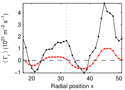
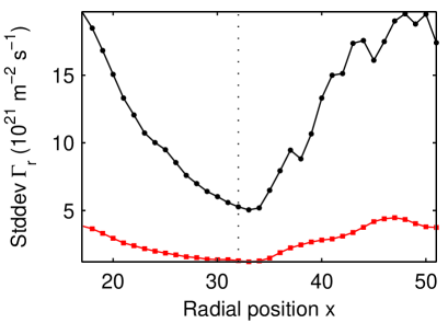
Figure 16: (a) Radial profiles of the time averaged particle flux $\langle\Gamma_{\rm{r}}\rangle$, (b) standard deviation $\rm{Stddev}(\Gamma_{\rm{r}})$ during the IBM blowout ($29.1\,\mathrm{\mu s}--97.3\,\mathrm{\mu s}$). Real values are plotted as red line with squares, measured values as black line with circles

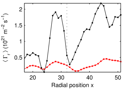
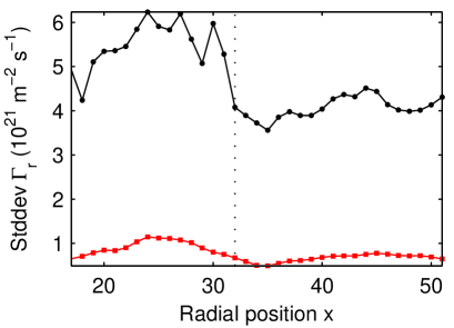
Figure 17: (a) Radial profiles of the time averaged particle flux $\langle\Gamma_{\rm{r}}\rangle$, (b) standard deviation $\rm{Stddev}(\Gamma_{\rm{r}})$ after the IBM blowout ($97.3\,\mathrm{\mu s}--239.5\,\mathrm{\mu s}$). Real values are plotted as red line with squares, measured values as black line with circles

The larger amplitudes of $\Gamma_{\rm{r}}^{\rm{m}}$ compared to $\Gamma_{\rm{r}}^{\rm{real}}$ can be observed at most positions in the radial profiles of mean values and standard deviations. The ratios between measured and real values are approximately comparable to the values given in the L-mode section. As shown in fig. 16, $\langle\Gamma_{\rm{r}}^{\rm{m}}\rangle$ and $\langle\Gamma_{\rm{r}}^{\rm{real}}\rangle$ differ at some radial positions not only in absolute values but also in sign, which is a significant distortion of the actual situation. However, the respective mean values are based only on a relatively small time interval and should not be overemphasised. Interestingly, the fluctuation amplitudes and the standard deviation of $\Gamma_{\rm{r}}^{\rm{m}}$ and $\Gamma_{\rm{r}}^{\rm{real}}$ approach a local minimum near the separatrix. This is especially pronounced during the blowout (fig. 16), but is still present afterwards (fig. 17).

As our simulation code can only provide data for the temporal evolution of one single IBM blowout and its aftermath, the fluctuations covered by the time series are not sufficient to allow a more detailed statistical analysis including probability density functions and statistical moments.

IV Conclusions

From the above investigations can be concluded, that neglecting any temperature fluctuations in our computations of probe measurements results in significant differences between the synthetically measured values and the actual quantities at all radial positions of the simulation domain, both in a saturated L-mode situation and in simulations of an IBM blowout. This holds especially for the floating potential and its use in calculations of the fluctuation induced particle flux. The latter shows a considerable discrepancy not only in the temporal evolution but also in statistical properties, if spatial variations of the temperature fluctuations are not taken into account. However, fluctuations of the electron temperature seem to be of much greater importance than ion temperature fluctuations.

Compared to the saturated L-mode situation, the investigation of time series involving an IBM blowout did not yield a major alteration of the ratio between real and measured quantities, apart from unsurprising changes due to the large peaks.

Although a realistic implementation of a virtual Langmuir probe in terms of geometry and particle processes would require the use of a kinetic model, the results from our gyrofluid simulations can nevertheless be regarded as relevant for experimental measurements, as all comparisons are performed within the simulation. In this respect they may serve as an indication to the particular importance of electron temperature fluctuations, whose neglect in evaluations of experimental data might lead to substantial deviations from the actual quantities.

References

- (1) Schrittwieser R et al. 2002 Plasma Phys. Contr. Fusion 44 567-578
- (2) Hutchinson I H 2002 Principles of Plasma Diagnostics (Cambridge: Cambridge University Press)
- (3) Stangeby P C 1982 J. Phys. D: Appl. Phys. 15 1007
- (4) Stangeby P C and McCracken G M 1990 Nucl. Fusion 30 1225
- (5) Mueller H W, Adamek J, Horacek J, Ionita C, Mehlmann F, Rohde V, Schrittwieser R and the ASDEX Upgrade Team 2010 Contrib. Plasma Phys. 50 847-853
- (6) Schubert M, Endler M and Thomsen H 2007 Rev. Sci. Instrum. 78 053505
- (7) Hidalgo C 1995 Plasma Phys. Contr. Fusion 37 A53-A67
- (8) Hidalgo C, Balbín R, Pedrosa M A, García-Cortés I and Ochando M A 1992 Phys. Rev. Lett. 69 1205
- (9) Chen S L and Sekiguchi T 1965 J. Appl. Phys. 36 2363
- (10) Xu Y et al. 2007 Nucl. Fusion 47 1696-1709
- (11) Boedo J A, Gray D, Conn R W, Luong P, Schaffer M, Ivanov R S, Chernilevsky A V, Van Oost G and the TEXTOR Team 1999 Rev. Sci. Instrum. 70 2997
- (12) Boedo J A, Terry P W, Gray D, Ivanov R S, Conn R W, Jachmich S, Van Oost G and the TEXTOR Team 2000 Phys. Rev. Lett. 84 2630
- (13) Rudakov D L, Boedo J A, Moyer R A, Lehmer R D, Gunner G and Watkins J G 2001 Rev. Sci. Instrum. 72 453
- (14) Schrittwieser R, Ionita C, Balan P, Silva C, Figueiredo H, Varandas C A F, Rasmussen J J and Naulin V 2008 Plasma Phys. Contr. Fusion 50 055004
- (15) Horacek J et al. 2010 Nucl. Fusion 50 105001
- (16) Adamek J et al. 2010 Contrib. Plasma Phys. 50 854-859
- (17) Adamek J, Duran I, Hron M, Stoeckel J, Balan P, Schrittwieser R, Ionita C, Martines E, Tichy M and Van Oost G 2002 Czech. J. Phys. 52 1115-20
- (18) Kirk A, Mueller H W, Herrmann A, Kocan M, Rohde V, Tamain P and the ASDEX Upgrade Team 2011 Plasma Phys. Contr. Fusion 53 035003
- (19) Scott B D 2006 Contrib. Plasma Phys. 46 714-725
- (20) Scott B D 2005 Phys. Plasmas 12 102307
- (21) Kendl A, Scott B D and Ribeiro T 2010 Phys. Plasmas 17 072302
- (22) Ribeiro T and Scott B D 2005, Plasma Phys. Contr. Fusion 47 1657-1679
- (23) Ribeiro T and Scott B D 2008, Plasma Phys. Contr. Fusion 50 055007
- (24) Scott B D 2001 Phys. Plasmas 8 447
- (25) Beer M A and Hammet G W 1996 Phys. Plasmas 3 4046
- (26) Carreras B A, Hidalgo C, Sánchez E, Pedrosa M A, Balbín R, García-Cortés I, Van Milligen B, Newman D E and Lynch V E 1996 Phys. Plasmas 3 2664-72
- (27) Zweben S J, Boedo J A, Grulke O, Hidalgo C, LaBombard B, Maqueda R J, Scarin P and Terry J L 2007 Plasma Phys. Contr. Fusion 49 S1-23
- (28) Nielsen A H, Pécseli H L and Rasmussen J J 1996 Phys. Plasmas 3 1530-44
- (29) Endler M, Niedermeyer H, Giannone L, Holzhauer E, Rudyj A, Theimer G, Tsois N and the ASDEX Team 1995 Nucl. Fusion 35 1307