Abstract

We study the bipartite entanglement of strongly correlated systems using exact diagonalization techniques. In particular, we examine how the entanglement changes in the presence of long-range interactions by studying the Pariser-Parr-Pople model with long-range interactions. We compare the results for this model with those obtained for the Hubbard and Heisenberg models with short-range interactions. This study helps us to understand why the density matrix renormalization group (DMRG) technique is so successful even in the presence of long-range interactions. To better understand the behavior of long-range interactions and why the DMRG works well with it, we study the entanglement spectrum of the ground state and a few excited states of finite chains. We also investigate if the symmetry properties of a state vector have any significance in relation to its entanglement. Finally, we make an interesting observation on the entanglement profiles of different states (across the energy spectrum) in comparison with the the corresponding profile of the density of states. We use isotropic chains and a molecule with non-Abelian symmetry for these numerical investigations.

1 Introduction

Quantum entanglement, which began with the famous EPR controversy [1], has become one of the most exciting and important fields of research in recent times. Stated simply, entanglement is the quantum correlation among different parts of a many-body system. It is a property of a quantum state and does not have any classical counterpart. It signifies that when a quantum system consists of two parts, one part is correlated with the other part even when the two parts are far apart and not ‘physically’ connected. Besides being fundamentally important in understanding or interpreting quantum mechanics, there are three main motivations for considering entanglement seriously [2]; it can be used to study the quantum-to-classical transition, it can be used for studying quantum phase transitions, and it has the potential to play a significant role in modern technology. Entanglement is at the heart of quantum computation and quantum communication which may be viewed as the future of computation and communication science.

In this paper, we will study the entanglement of a number of many-body systems in order to characterize and better understand the eigenstates of a many-body Hamiltonian. A wide range of entanglement studies have already been carried out on many-body systems [3], but to the best of our knowledge, the role of long-range interactions has not been investigated. Unlike many of the other studies of many-body systems, we will not try to find the scaling properties of entanglement with the system size; instead, we will make a comparative study of finite systems to understand the relative behaviors of different interacting models. The Pariser-Parr-Pople (PPP) Hamiltonian with standard parameters, the Hubbard Hamiltonian with different values of the on-site interaction and the antiferromagnetic Heisenberg Hamiltonian with both spin 1/2 and 1 sites will be used for our comparative studies. The investigations will be done for the ground states of chains with either varying lengths (with equal block sizes) or varying block sizes (with fixed chain length). In the case of the interacting electron systems, we will also study a few important excited states such as $1^{1}A_{g}^{+}$, $2^{1}A_{g}^{+}$, $1^{1}B_{u}^{-}$ and $1^{3}B_{u}^{+}$. These correspond to the important states of a conjugated polymer, namely, the ground state ($1^{1}A_{g}^{+}$), the lowest energy two-photon state ($2^{1}A_{g}^{+}$), the lowest energy one-photon state ($1^{1}B_{u}^{-}$), and the lowest energy triplet state ($1^{3}B_{u}^{+}$). The labels ‘$A$’ and ‘$B$’ correspond to even and odd parity states under reflection of the chain. For linear chains these are also even or odd under inversion, and hence the subscript ‘$g$’ goes with ‘$A$’ state and ‘$u$’ with ‘$B$’ states. The superscript ‘+’ or ‘-’ refers to even or odd states under electron-hole symmetry. The ‘+’ space includes ‘covalent’ many-body basis states with one electron per site, while ‘ionic’ space excludes these states. To better understand the effect of long-range interactions, we will also study the entanglement spectrum of the ground state of a chain. A comparison will be done with the results for the short-range interacting Hubbard model (with $U/t=4$).

Our study serves the important purpose of understanding the high accuracy of density matrix renormalization group (DMRG) technique [4] when applied to the PPP model, even though it incorporates long-range electron-electron interactions. The success of the DMRG method in low-dimensional systems is attributed to the connection between the area law of the entanglement entropy, $S$ [5, 6], and the cut-off, $m$, in the number of density matrix eigenvectors (DMEVs) that should be retained in a DMRG calculation for a given accuracy. The entanglement entropy of a system surrounded by an environment scales as the area between the system and the environment. The cut-off in the number of DMEVs for a fixed accuracy scales exponentially with the entanglement entropy ($m\sim 2^{S}$) [4]. However, one-dimensional systems away from criticality have a constant entanglement entropy independent of the size of the system. This explains why the DMRG method is so successful in studying correlated one-dimensional systems. It also underlines the difficulties with the DMRG technique in studying higher dimensional systems as well as one-dimensional systems close to criticality; the latter systems have a logarithmic correction to the entropy which leads to an increase in the entanglement entropy as one approaches the critical point. The area law arises due to the dangling bonds which are created by cutting the system from the environment. This would seem to imply that when we have systems with long-range interactions, even in one dimension the DMRG method should not retain the same accuracy for a given cut-off as the system size is increased because the number of interactions that are cut resulting in dangling bonds increases with increasing system size. However, DMRG calculations on quasi-one-dimensional systems with diagonal long-range interactions have proved to be very accurate. Our entanglement study of one-dimensional systems is aimed at understanding this feature.

We will also investigate the entanglement properties of a 12-site icosahedral system using the PPP Hamiltonian. This system has the largest non-Abelian point group symmetry; this enables us to examine the role of spatial and spin symmetries in the entanglement of a state. In this context, we will explicitly discuss the issue of degeneracies, noting that the entanglement obtained for different degenerate states are not the same. Additionally, for both the chain and icosahedral systems, a comparative study will be made between the entanglement profiles (across the energy spectrum) and the corresponding profile of the density of states (DoS) leading to some interesting observations.

In the next section (Sec. 2), we will first discuss the theoretical background of our work where we discuss the measure of bipartite entanglement for pure states. Subsequently, we will introduce the different Hamiltonians used and the numerical techniques employed. In Sec. 3, we will present and discuss our results, first for chains and then for the icosahedral system. At the end of this section, we will compare the entanglement profiles with the corresponding DoS profiles. We will then conclude our work with some remarks on our observations.

2 Theoretical Background and Numerical Techniques

In this section we will briefly describe the entanglement measure, the Hamiltonians for strongly correlated systems and the numerical techniques used in this work.

2.1 The Entanglement Measure

In the introductory section we introduced the notion of entanglement intuitively. In a more formal language, the bipartite entanglement for pure states is defined as follows. Two parts of a system are said to be entangled in a particular state if the corresponding wave function of the total system cannot be expressed as a direct product of some states of the two parts. Similar definitions can be given for the bipartite entanglement of mixed states and also for the multipartite entanglement of both pure and mixed states, but we will not be interested in these in the present work. Quantifying entanglement is generally non-trivial and can have different measures according to the usefulness in different contexts [3, 7]. Fortunately, bipartite entanglement for pure states has a well defined and simple measure, namely, the von Neumann entropy which is given by

$$S=-Tr~{}(\rho~{}{\rm log_{2}}~{}\rho),$$ (1)

where $\rho$ is the reduced density matrix of either one of the two parts, ‘Tr’ implies tracing over an operator (or matrix), and ‘log’ is the logarithm which is conventionally calculated with base 2. If $w_{i}$’s are the eigenvalues of $\rho$, then $S$ can be written as

$$S=-\sum_{i}~{}w_{i}~{}{\rm log_{2}}~{}w_{i}.$$ (2)

Here we note that, $w_{i}\geq 0$ and $\displaystyle\sum_{i}w_{i}=1$. Now let $\displaystyle|\psi\rangle=\sum_{ij}C_{ij}|\phi_{i}\rangle^{l}|\phi_{j}\rangle^{r}$ be some pure state (say, an eigenstate of a given Hamiltonian), where $|\phi_{i}\rangle^{l}$s and $|\phi_{i}\rangle^{r}$s are the normalized basis states of the two parts (conveniently called the left and right parts) of a system. Then the elements of the reduced density matrix of the left part are given in terms of $C_{ij}$ by

$$\rho_{ij}=\sum_{k}C_{ik}C_{jk}^{*},$$ (3)

with ‘*’ implies complex conjugation. Alternatively, one can consider the reduced density matrix of the right part whose matrix elements are given by

$$\rho^{\prime}_{ij}=\sum_{k}C_{ki}C_{kj}^{*}.$$ (4)

The dimensionalities and hence the number of eigenvalues of $\rho$ and $\rho^{\prime}$ can be quite different from each other. However, it can be shown, using the Schmidt singular value decomposition, that the non-zero eigenvalues of $\rho$ and $\rho^{\prime}$ are always equal to each other; hence the von Neumann entropy given in Eq. (2) is the same regardless of whether it is calculated using the eigenvalues of $\rho$ or $\rho^{\prime}$.

2.2 Interacting Model Hamiltonians

A number of model Hamiltonians for strongly correlated systems will be used in this study. The Pariser-Parr-Pople (PPP) model Hamiltonian, which includes interactions between distant neighbors in addition to on-site interactions, is given by

$${\hat{H}}~{}=~{}-\sum_{<ij>,\sigma}t_{ij}(\hat{c}^{\dagger}_{i\sigma}\hat{c}_{j\sigma}~{}+~{}H.c.)~{}+~{}\sum_{i}\frac{U_{i}}{2}\hat{n}_{i}(\hat{n}_{i}-1)~{}+~{}\sum_{i>j}V_{ij}(\hat{n}_{i}-z_{i})(\hat{n}_{j}-z_{j}).$$ (5)

Here, the first term of the Hamiltonian is the nearest-neighbor transfer term also called the Hückel term, with $\hat{c}_{i\sigma}^{~{}\dagger}$ ($\hat{c}_{i\sigma}$) creating (annihilating) an electron with spin $\sigma$ at the $i^{th}$ site, and the summation is over a bonded pair of sites $<ij>$ (in our case nearest neighbors). The second term is the Hubbard term with $U_{i}$ being the on-site repulsion energy for the $i^{th}$ site; here $\hat{n}_{i}=\sum_{\sigma}c^{\dagger}_{i\sigma}c_{i\sigma}$ denotes the number operator for the $i^{th}$ site. The Hamiltonian with only the first term described the one-band tight-binding model or the Hückel model while inclusion of the second term gives the Hubbard Hamiltonian [8]. The third term brings in the effects of long-range interactions, where $V_{ij}$ is the density-density electron repulsion integral between sites $i$ and $j$, $z_{i}$ is the local chemical potential given by the occupancy of the $i^{th}$ site for which the site is neutral. This term was first introduced for conjugated $\pi$ electronic systems, by Pariser and Parr [9] as well as by Pople [10] independently in 1953. We employ the Ohno interpolation scheme (applicable to conjugated systems) to parametrize $V_{ij}$ [11],

$$V_{ij}=14.397\left[\left(\frac{28.794}{U_{i}+U_{j}}\right)^{2}+r_{ij}^{2}\right]^{-1/2}.$$ (6)

Here $r_{ij}$ is the distance (in Å ) between the $i^{th}$ and $j^{th}$ sites and the energies are in eV. One uses $t=-2.4$ eV and $U=11.26$ eV as the standard parameters for the PPP Hamiltonian of a conjugated system. In the large $|U/t|$ limit, Hamiltonian in Eq. (5) reduces to an isotropic spin Hamiltonian (the Heisenberg Hamiltonian). The Heisenberg Hamiltonian with site spin $\vec{S}_{i}$ at the $i^{th}$ site can be written as,

$$H=\sum_{<ij>}J_{ij}\vec{S}_{i}\cdot\vec{S}_{j},$$ (7)

where $J_{ij}$ is the exchange coupling constant between sites $i$ and $j$.

2.3 Numerical Techniques

For one-dimensional electronic systems we will use the Rumer-Pauling valence bond (VB) basis, which is spin-adapted and complete but non-orthogonal [12, 13]. The $C_{2}$ symmetry and electron-hole symmetry are applied to break the spin adapted space (only singlets and triplets are considered in our study) into four symmetry adapted subspaces, namely, $A_{g}^{+}$, $A_{g}^{-}$, $B_{u}^{+}$ and $B_{u}^{-}$ [14, 16]. Once we diagonalize a Hamiltonian in some particular space, we get eigenstates which are linear combinations of symmetrized VB basis states. These eigenstates can be expressed as linear combination of the initial VB basis (unsymmetrized) states. We can also expand the VB basis states into linear combination of basis states with a constant values of $M_{S}$ (i.e., $S_{z}$) [14, 15], and can thus express the eigenstates as linear combinations of states with a particular value of $M_{S}$. This constant $M_{S}$ basis conserves the $z$-component of the total spin and being orthonormal, it is convenient to use in our study. For spin chains (both spin-1/2 and spin-1), we only studied the ground state to compare them with those from the electronic models. We also recently developed a hybrid VB-constant $M_{S}$ basis technique, which can exploit both spin and spatial symmetries of an arbitrary point group [15, 17]. Here the eigenstates are automatically obtained as linear combinations of constant $M_{S}$ basis. We used this hybrid method for the entanglement study of a half-filled 12-site icosahedral system (see Fig. 8) which has a huge Hilbert space (with dimension 1,778,966) [15]. Once we get an eigenstate as a linear combination of constant $M_{S}$ basis, we can use Eq. (3) to compute the reduced density matrices. These matrices can be diagonalized to obtain the eigenvalues and subsequently the entropy using Eq. (2). In Table (2) we show the dimensionalities of different spin and spatial symmetry adapted subspaces of the icosahedral system. These dimensionalities have some significance related to the entropy profiles of different subspaces; this will be discussed in Sec. 3.2.

Since all our results will be interpreted in terms of the VB basis, we give a very brief description of the basis [13]. For spin systems, the spin of a magnetic site “$s_{i}$” is replaced by $2s_{i}$ spin-half objects. Now to obtain a state with total spin $S$ from $N$ such spin-1/2 objects from all the magnetic centers of the system, a total of $2S$ such objects are left unpaired and the remaining $N-2S$ of the spin-1/2 objects are singlet spin paired explicitly, subject to the following restrictions: (i) there should be no singlet pairing of any two spin-half objects belonging to the same magnetic center (this ensures that the $2s_{i}$ objects are in a totally symmetric combination), (ii) when all the spin-half objects are arranged as $N$ dots on a regular $N$-sided polygon and lines are drawn between spin paired objects, there should be no intersecting lines in the diagram, and (iii) these lines should not enclose any unpaired spin-1/2 objects which are connected by an arrow when all the sites are aligned on a straight line and the VB diagram is drawn such that all singlet lines are above this straight line. These rules follow from the generalization of the Rumer-Pauling rules to objects with spin greater than 1/2 and total spin greater than zero. The set of diagrams which obey these rules are called “legal” VB diagrams (or basis states). All legal VB diagrams form a complete and linearly independent set. VB diagrams which do not follow these rules are called “illegal” and can be expressed as linear combination of “legal” diagrams. Note that for an odd number of spin-1/2 objects and total spin $S=1/2$, we cannot have an arrow. In this case we add a $``phantom”$ site and generate singlet diagrams; the phantom site does not appear in the Hamiltonian.

For electronic systems, a given orbital can be in one of four states; it can be (1) empty, (2) singly occupied with an up-spin electron, (3) singly occupied with a down-spin electron, and (4) doubly occupied. Let $N$ be the number of orbitals, $N_{e}$ be the number of electrons with $N_{\uparrow}$ up-spin electrons and $N_{\downarrow}$ down-spin electrons, so that $N_{e}=N_{\uparrow}+N_{\downarrow}$. Now, for a fixed occupancy of the orbitals, a linearly independent and complete set of states with total spin $S$ and $M_{S}=S$ is obtained by the extended Rumer-Pauling rules as follows. (i) The $N$ orbitals are arranged as dots along a straight line. (ii) Doubly occupied sites are marked as crosses. (iii) An arrow is passed through $2S$ of the singly occupied sites, passing on or above the straight line on which the system is represented. The arrow denotes the spin coupling corresponding to total spin $S$ and total $z$-component $M_{S}=S$. VB diagrams corresponding to other $M_{S}$ states can be obtained by operating on the arrow with the $S^{-}$ operator the required number of times. (iv) Remaining singly occupied sites are singlet paired and are denoted by lines drawn between them. (v) Diagrams with (a) two or more crossing lines, or (b) crossing line and the arrow, or (c) a line enclosing the arrow are called “illegal” and are rejected. The remaining set of diagrams correspond to a complete and linearly independent set of VB states for the chosen orbital occupancy. The set of VB diagrams which obey the extended Rumer-Pauling rules are called “legal” VB diagrams. Note that for $N_{e}$ odd and total spin $S=1/2$, we cannot have an arrow. As with the pure spin case, we handle this situation by the concept of a $``phantom"$ site.

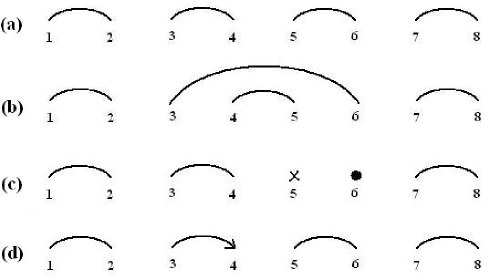
Figure 1: Some legal VB diagrams are shown for an 8-site system. The first three diagrams, (a), (b) and (c), are for total spin zero while the last one, (d), is for total spin one. Diagram (c) is possible only for electronic systems.

Some legal diagrams are shown in Fig. 1; these will be referred to in the next section.

Before finishing this section let us stress two important points: (i) the procedure above will give us states with $M_{S}$ equal to the total spin $S$, and (ii) any basis (a diagram) can be written as a direct product of states of lines (representing singlets), arrow (representing the spin of the diagram) and crosses (representing doubly occupied sites) in any order. Since each of the objects contain a pair of fermionic operators, those operators commute. Note, crosses or dots do not appear for pure spin systems. If we calculate the entropy for a VB diagrammatic basis, it would give a non-zero value only if the boundary plane dividing the system into two parts (left and right) intersects at least one line of the diagram. If the boundary plane intersects only an arrow (if present), it would give zero entropy as the arrow is the direct product state of all the unpaired spins (or electrons) as we have chosen $M_{S}=S$. To clarify this we note that in diagram (a) of Fig. 1, if the boundary plane intersects the system in between sites 3 and 4, the calculated entropy will not be zero; on the other hand, when the plane intersects the system in between sites 4 and 5, the calculated entropy will be zero. Since the eigenstates of a system can be written as linear combination of VB diagrams, the entropy calculated for an eigenstate would be high if the leading VB diagrams (with large coefficients) themselves have non-zero entropy.

3 Results and Discussion

In this section, we first present results for spin and electronic system for the chains. We follow this with results and discussions for the icosahedral cluster. In the last part of the section, we compare and discuss the DoS profiles with the corresponding entanglement profiles for different spaces of both the chain and icosahedral systems.

3.1 Entanglement Studies of Chains

We have performed entanglement studies on the chain system mainly to explore the effect of long-range interactions. In these studies we will also see the role of the chain length and block size on the entanglement entropy. For this purpose we study Hubbard chains (with $U/t=$ 0, 2, 4, 6, 8, 12 and 40) and PPP chains. Electronic systems are always taken to be half-filled. We also study the entanglement of spin-1/2 and spin-1 Heisenberg antiferromagnetic spin chains in order to compare its size dependence with the results for electronic systems.

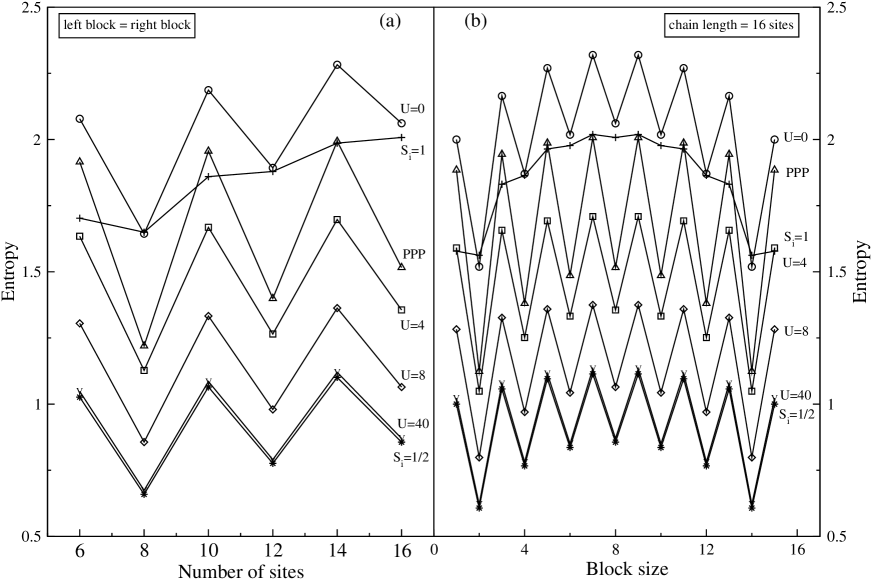
Figure 2: (a) Ground state entanglement studied with equal block sizes and increasing chain length. (b) Ground state entanglement studied with different block sizes for a fixed chain length (16 sites).

First we study the entanglement in the ground state of different models, with respect to variations in both the chain length and the block size (see Fig. 2). We find that for the electronic systems, for odd block sizes (having an odd number of sites), the entropy is high, while for even block sizes the entropy is low. This can be explained from the VB theory. In the ground state of a chain, the contribution of the Kekule basis states (see Fig. 1 a), is large since this basis state corresponds to nearest-neighbor singlets. Now depending on the position of the boundary plane (whether it intersects a singlet line or not; see the discussion in Sec. 2.3), the entropy of the ground state will be high or low. This is the reason why for equal block sizes, the $4n+2$ ($n$ being a positive integer) chains have higher entropy than the $4n$ chains; in the former, we cut a singlet line in the Kekule diagram while in the latter, the system is divided between nearest-neighbor lines of the Kekule diagram (see Fig. 2 a). In order to further verify this odd-even effect, we also studied 16-sites fermionic chains, with different sizes of blocks (see Fig. 2 b). Here, we find that the entropy is large (small) whenever it has an odd (even) number of sites in a block.

In this regard we also note that the odd-even effect is more prominent or sharper for the PPP model compared to that for the Hubbard model. This is because the PPP term (the third term in Eq. (5)) is a diagonal interaction term between empty and doubly occupied sites. The lines or arrow (singly occupied sites) remain unchanged by the term. This signifies that the long-range term favours ionic states; as a result, the number of covalent states (as in Fig. 1 b) present in the ground state is less compared to the case of the Hubbard model. Now due to dominance of diagrams like in Fig. 1 a among the other less important covalent diagrams present in the ground state (anyway ionic diagrams contribute less towards entropy due to lack of lines), odd-even effect becomes sharper for the PPP model.

We further notice that, within the even or odd block sizes, the entropy increases as shown in Fig. 2 a and it takes a dome-like structure as shown in Fig. 2 b. This is because the entropy of a system generally increases with the Schmidt number (coming from the Schmidt decomposition). As this number grows as the minimum of the Fock space dimensions of two blocks, in the first case (Fig. 2 a) it increases linearly with the system size and in the second case (Fig. 2 b) it is maximum when the block sizes are the same.

Another important observation for the Hubbard system is that the entropy decreases with increasing $U/t$. This is because an increase in $U/t$ leads to a smaller contribution from the ionic functions to the ground state. This effectively reduces the number of states involved (or equivalently the Schmidt number), which results in a decreased entropy. This fact is further supported by the result that the entropy profile for the Hubbard chain approaches that of the spin-1/2 antiferromagnetic Heisenberg spin chain with increase in $U/t$. We remember here that the ground state of the spin chain is dominated by the Kekule states.

In order to study the entanglement behavior of spin systems and compare the result with the corresponding behavior of electronic systems, we have also studied the entropy in the ground state of the spin-1/2 and spin-1 Heisenberg spin chains. Firstly, we note that the entropy profile of the spin-1/2 chain closely matches that of the Hubbard chain with $U/t$ = 40, and it exhibits a strong odd-even effect. The entropy of the spin-1 chain, on the other hand, shows a very weak odd-even effect. The magnitude of the entropy is higher in all cases compared to the spin-1/2 chain due to the large Fock space dimensionality of the spin-1 chain (note that a spin-1 can be considered as two spin-1/2’s without the singlet combinations between them). The weakness of the odd-even effect in the spin-1 chain implies that not only the Kekule states, but also other VB basis states (where singlets form between distant sites) contribute significantly to the ground state.

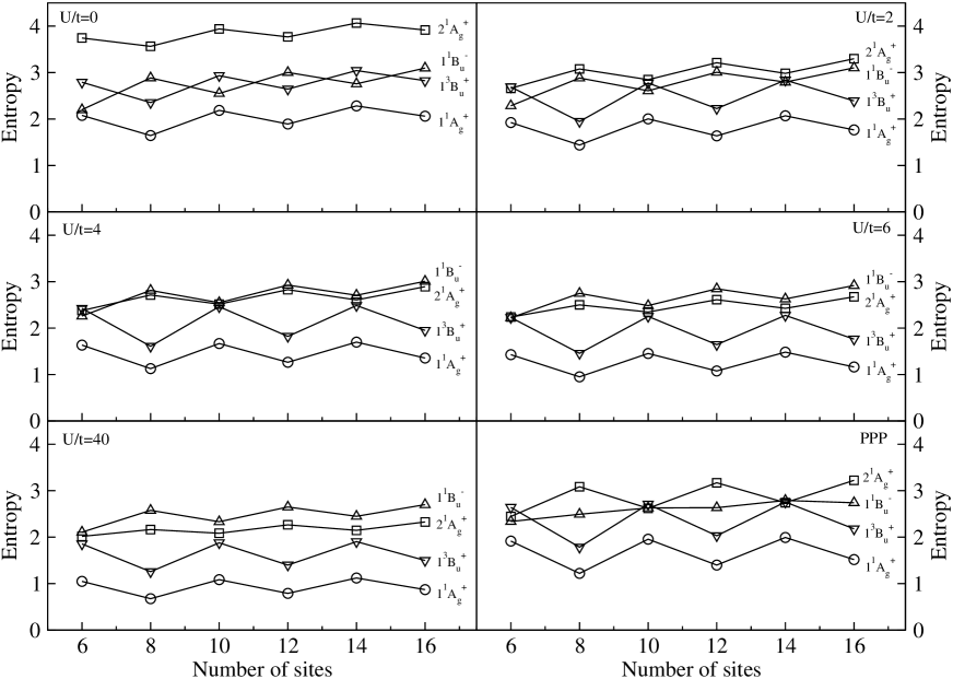
Figure 3: Entropy for some important excited states (along with the ground state) are shown here as a function of chain length (equal block size). Values shown here are for the Hubbard model with $U/t$ = 0, 2, 4, 6, 40, and for the PPP model.

We also study the entanglement for some important excited states of the Hubbard model for different $U/t$ values and the PPP model (see Fig. 3). Here we find that the entropy for 2${}^{1}A_{g}^{+}$ (lowest energy two-photon singlet state) is higher compared to the other states considered when $U$ =0. This is due to the fact that its energy is higher compared to others, hence it has a greater admixture of basis states like the ones shown in Fig. 1 b. Since these basis states contain singlet lines between distant neighbors, the state has a high entropy. However, the entropy of this state decreases as $U$ increases. This is because as $U/t$ increases, the 2${}^{1}A_{g}^{+}$ state becomes the spin wave excitation of a spin-1/2 Heisenberg antiferromagnetic chain. As already discussed, the entropy of spin chains is smaller than that of the fermionic chains. We also find that the odd-even effect in this state is smaller compared to the other states in the Hubbard model while the effect is nearly absent in the $1^{1}B_{u}^{-}$ state of the PPP model. This observation in the Hubbard model can be understood from the fact that the $2^{1}A_{g}^{+}$ state is composed of two triplets. These triplets tend to be separated. This implies that in the half-blocks, the favored states correspond to large spin and hence the odd-even effect will be less pronounced. The absence of the odd-even effect in the $1^{1}B_{u}^{-}$ state for the PPP model can also be understood from the fact that in the one-photon state, purely covalent basis states are absent, and that the PPP term favors basis states with more ion-pairs. Since there are many such ionic basis states present in significant amounts in this state, the odd-even effect will be suppressed here. We further notice that the odd-even effect reverses for $2^{1}A_{g}^{+}$ state when one goes from $U=0$ to even a small value (we have taken $U=2$ here). An understanding of this feature requires further analysis.

To better understand the dome-like structure of the entropy across the energy spectrum, we histogram the number $n_{p}(\rho)$ of density matrix eigenvalues in the range $10^{-p}>\rho>10^{-(p+1)}$ and plot it against the negative logarithm of eigenvalues $-{\rm log_{2}}\rho$. These are shown for states from the spaces $1^{1}A_{g}^{+}$, $1^{1}B_{u}^{-}$ and $1^{3}B_{u}^{+}$ in Figs. 4, 5 and 6 respectively. From the profiles we note that for states with very low and very high energies, the histograms have a broader distribution, while the states in the middle of the energy spectrum have a narrow distribution (having large $n(\rho)$) and are centered towards the origin of the axis. It is clear from Eq. (2), that this distribution leads to a large entropy for the states with intermediate energies and a small entropy for states at either end of the energy eigenvalue spectrum.

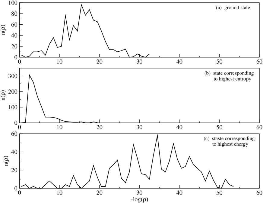
Figure 4: DoS profiles of eigenvalues of reduced density matrix (RDM) for three different states from the ${}^{1}A_{g}^{+}$ space. The result is obtained for the half-filled 10-site chain using the PPP Hamiltonian.

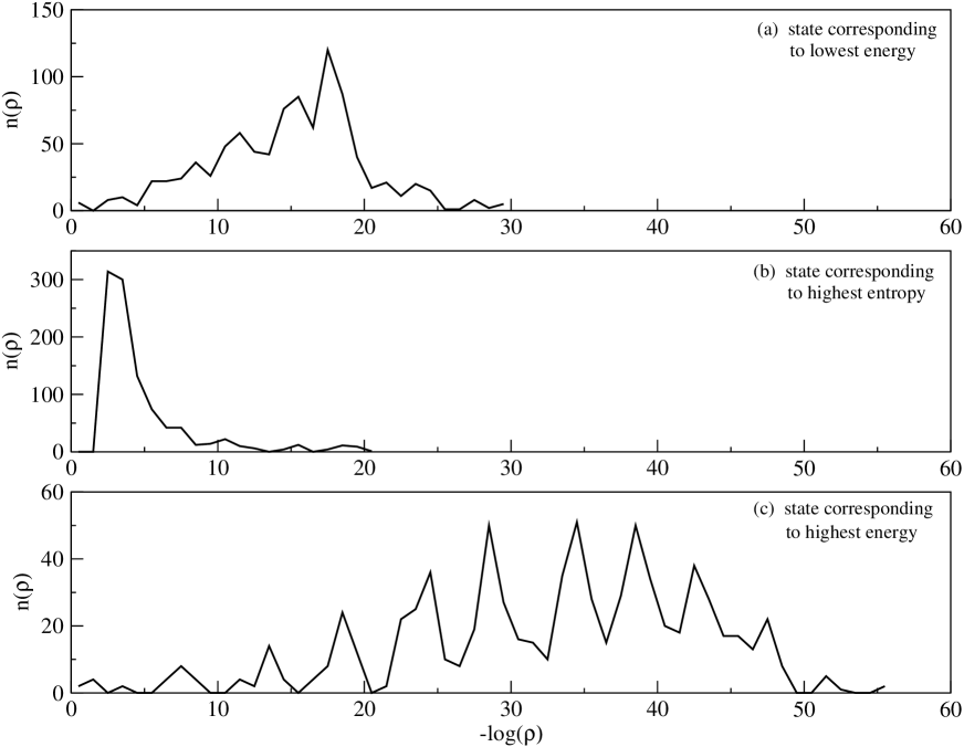
Figure 5: DoS profiles of eigenvalues of RDM for three different states from the ${}^{1}B_{u}^{-}$ space. The result is obtained for the half-filled 10-site chain using the PPP Hamiltonian.

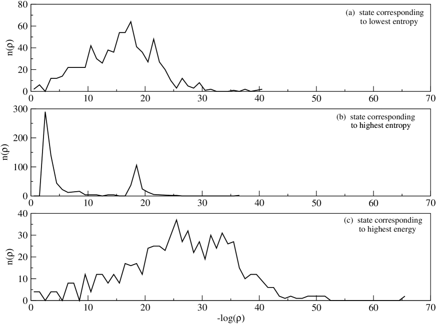
Figure 6: DoS profiles of eigenvalues of RDM for three different states from the ${}^{3}B_{u}^{+}$ space. The result is obtained for the half-filled 10-site chain using the PPP Hamiltonian.

Our results also show why the DMRG technique is so successful for the one-dimensional PPP model even though the model has long-range interactions. Note that the long-range interactions renders the system topologically higher dimensional since cutting the system leads to dangling bonds whose number increases with increasing system size; hence, according to the area law, the cut-off in the number of DMEVs for a fixed accuracy should increase with the system size. But we can see from Fig. 2 that, even though the odd-even effect is sharper for the PPP model compared to different short-range models, the change of the entropy with the system size is essentially the same as for the short-range models. This can be understood in the following way: the long-range part of the PPP Hamiltonian in Eq. (5) involves diagonal interactions between sites which are empty or doubly occupied. This term only weakly affects the weightage of states with large single occupancies (i.e., lines and arrow, in the VB language). Since the covalent states (lines) which actually contribute towards the entropy are not significantly affected by this long-range term, the overall entropy of an eigenstate does not change much. The only consequence of this term is the sharper odd-even effect which results, as we already explained, due to the dominance of diagrams like in Fig 1 a in the ground state of the PPP model.

To further substantiate our claim that the long-range interactions do not affect the entanglement entropy significantly, we have considered the the ground state and a few excited states of a chain of 10 sites in the PPP and Hubbard models and calculated the entanglement entropy within different sectors of total electron numbers and $z$-component of total spin for one half of the system. The idea of an entanglement spectrum was introduced in Ref. [18], and it has proved to be very useful for studying a number of strongly correlated quantum systems; in that work, the entanglement spectrum was obtained by calculating $-log_{2}(w_{i})$ for all the eigenvalues of the reduced density matrix in different sectors corresponding to the values of various additive quantum numbers (i.e., eigenvalues of conserved quantities whose values for the entire system are equal to the sum of their values for the two parts of the system). In the same spirit, we have separated out the contributions of the different total $S_{z}$ and $n$ sectors, where the former corresponds to the $z$ component of the total spin and the latter to the number of electrons in the part of the chain for which we compute the entanglement entropy; within each of these sectors, we have calculated the sum $-\sum_{i}w_{i}{\rm log_{2}}w_{i}$ (instead of $-{\rm log_{2}}w_{i}$ as was done in Ref. [18]). The result is shown in Table 1. In Fig. 7 we show the DoS of the reduced density matrix for the PPP model in some sectors of $S_{z}$ and $n$. Due to the electron-hole and spin-inversion symmetries many sectors have the same DoS within the numerical accuracy.

Our results show that the entropy for different sectors are almost the same for long-range and short-range models. This supports our previous arguments about the reason for the success of the DMRG method for the PPP model.

Table 1: Entanglement spectrum for different sectors of total electron number $N_{e}$ and $z$-component of total spin $M_{s}$ for one half of the system. We present results for both PPP and Hubbard models (with $U/t=4$) for comparison.

Model	State	Sector		Entropy
		Ms	Ne
		0.5	5	0.557
		0.0	4	0.408
	Ag+	1.0	4	6.1x$10^{-3}$
		0.5	3	4.9x$10^{-4}$
		1.5	5	4.6x$10^{-4}$
		0.0	2	1.1x$10^{-8}$
		0.5	5	0.686
		0.0	4	0.576
PPP	Bu-	1.0	4	1.9x$10^{-2}$
		0.5	3	6.1x$10^{-3}$
		1.5	5	9.2x$10^{-5}$
		0.0	2	6.1x$10^{-7}$
		0.5	5	1.049
		-0.5	5	0.282
	3Bu+	1.5	5	0.282
		0.0	4	0.274
		1.0	6	0.274
		0.0	6	0.274
		0.5	5	0.545
		0.0	4	0.275
	Ag+	1.0	4	6.1x$10^{-3}$
		1.5	5	1.5x$10^{-3}$
		0.5	3	3.5x$10^{-4}$
		0.0	2	2.4x$10^{-8}$
		0.0	4	0.622
		0.5	5	0.445
Hubbard	Bu-	1.0	4	6.7x$10^{-2}$
(U/t = 4)		0.5	3	3.6x$10^{-2}$
		1.5	5	1.5x$10^{-4}$
		0.0	2	4.2x$10^{-5}$
		0.5	5	1.057
		1.5	5	0.345
	3Bu+	-0.5	5	0.345
		0.0	4	0.178
		1.0	6	0.178
		0.0	6	0.178

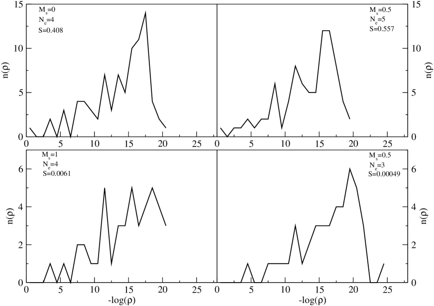
Figure 7: DoS profiles of eigenvalues of RDM for different sectors corresponding to different electron numbers and $z$-components of total spin. The state studied here is the ground state ($A_{g}^{+}$) of a 10-site chain using the PPP Hamiltonian.

3.2 Entanglement Studies of an Icosahedron

To learn if symmetries play any recognizable role in entanglement, we have studied a 12-site half-filled icosahedron with the Hamiltonian of the PPP model [15]. The first important issue here is of the degeneracies. In general, the entanglement is not the same for degenerate states, and a linear combination of two such states can give another degenerate state with a different entanglement. In the following we address this problem of non-unique entanglement of degenerate states.

Table 2: Dimensionalities of different symmetry and spin subspaces of a half-filled icosahedral cluster.

S${}_{tot}\rightarrow$
$\Gamma$ $\downarrow$	0	1	2	3	4	5	6
Ag	2040	3128	1684	382	38	3	1
T1g	16602	28821	14625	3261	309	6	0
T2g	16602	28821	14625	3261	309	6	0
Gg	30272	50932	26236	5880	568	16	0
Hg	47940	79305	41255	9220	900	40	0
Au	1852	3188	1644	348	40	0	0
T1u	17082	28686	14700	3372	294	18	0
T2u	17082	28686	14700	3372	294	18	0
Gu	30160	50992	26176	5888	560	16	0
Hu	46880	79680	40980	9060	900	20	0
Tot Dim $\rightarrow$	226512	382239	196625	44044	4212	143	1

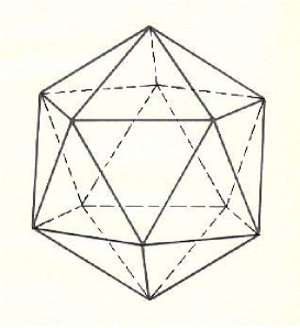
Figure 8: An icosahedron system of 12 sites is shown here. The upper six sites of the system constitute one part and the rest of the sites constitute the other part for our entanglement calculations.

For spin degeneracies (i.e., same total spin but different $M_{S}$ values) the problem is not severe. Since the $z$-component of the total spin is an observable, we can always choose one of its eigenstates. In our study we have chosen states with $M_{S}=S$.

The non-uniqueness problem cannot be trivially solved for the case of discrete symmetries. In this case we do not have any observable to select one of the degenerate states for our study. It is known that the projection operator to the full degenerate space is invariant. If $\rho_{i}$ is the density matrix of the $i^{th}$ state in a degenerate manifold, then the density matrix averaged over the $g$-fold degeneracy is given by $\rho_{av}=(1/g)~{}\sum_{i=1}^{g}~{}\rho_{i}$. This $\rho_{av}$ is invariant under a change of the basis states. To obtain the reduced density matrix, and subsequently the entanglement entropy, we take the upper half of the system (upper 6 sites of the Fig. 8) as one part and the rest as the other part.

The eigenstates of the Hamiltonian correspond to integer spins lying between 0 and 6 and belong to one of the ten irreducible representations of the icosahedral cluster. To see the role of symmetry, we calculate the entropy in different spatial symmetry subspaces for two chosen spin states 0 and 1. This is shown in Figs. 9 a and b. To see the effect of the spin, we calculate the entropy in different spin subspaces for two chosen spatial symmetries $A_{g}$ and $G_{u}$. This is shown in Figs. 9 c and d.

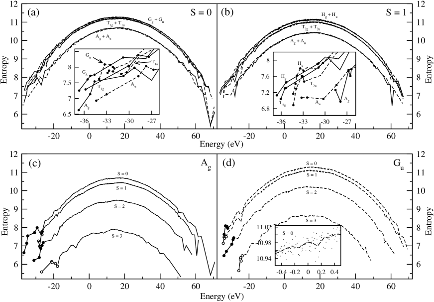
Figure 9: Entropy calculated across the energy spectrum of different subspaces. Insets of (a) and (b) show entropies (black dots) of the first few states of the corresponding subspaces. (c) and (d) show entropies of the first few states using filled circles (for even spins) and open circles (for odd spins). Inset of (d) shows how entropies fluctuate about a mean value. Solid lines represent plots for gerade ($g$) spaces and broken lines represent plots for ungerade ($u$) spaces.

Since the entropy profiles fluctuate (see inset of Fig. 9 d), we take averages to analyze the general features. The averaging is done in the following way: the first and last few states in the energy spectrum are comparatively well-separated from each other, we leave five of them from both sides with their actual values (which are zoomed in the insets of Fig. 9 a and b). Since the rest of the points from both sides of the spectrum are closely placed, we average the entropy over sets of four consecutive states. This is done for up to 40 states from both ends of the spectrum. Since the middle part of the spectrum is highly dense [19], we average the entropy values over 10 consecutive states. We find that the entropies for the lowest states in different symmetrized subspaces, for a given spin, do not seem to have any special features (see insets of Figs. 9 a and b). However, for a fixed spin, the maxima of the entropy profiles (see the middle portions of Figs. 9 a and b) are higher for degenerate spaces, such as $T$, $G$, and $H$ compared to the non-degenerate $A$ spaces. In fact, the higher the degeneracy in a space, the higher is the entropy maximum; for example, the $H$ space has a higher maximum entropy compared to, say, the $T$ space. This fact can be partially explained by the fact that spaces with a higher maximum entropy have a higher dimensionality (see Table 2). But this does not explain why the entropy of a non-degenerate space is much lower compared to the degenerate ones, while the degenerate ones are very close in entropy. Its explanation lies in the fact that entropy increases with DoS (see Sec 3.3) and DoS is much lower for non-degenerate spaces [15]. We also note that for a subspace with a particular spatial symmetry, the maxima of the entropy profiles is higher for lower spin spaces (see Figs. 9 c and d). This is also generally true for the entropy of the lowest states of different spins in a given spatial symmetry subspace. This can be qualitatively explained by the dimensionalities of the spaces. However, there must be other factors contributing to this observation since, in general, the entropy for triplet states is lower than that of the singlet states even though the dimension of the triplet space is higher than that of the singlet space. This fact can be explained by noting that the low-spin states are made up of more singlet pairs (lines) than the high-spin states, and we are only considering states with the highest $M_{S}$ value (i.e., $S$) which are least entangled. This leads to a higher entropy for states with a lower total spin. If we had worked with the $M_{S}=0$ state of the triplet states (which is a linear combination of two configurations), we would have expected a higher entropy for the states.

The entropy profiles are not monotonically increasing in each symmetry subspace; each profile reaches a maxima and then decreases. This can be explained by considering the properties of the VB basis. Initially, for the low-energy eigenstates, the VB states like Fig. 1 a appear with larger weights. This is because these VB states have nearest-neighbor singlets. These VB states would contribute less towards the entropy of an eigenstate, as the boundary plane crosses a smaller number of lines on the average. In higher energy eigenstates, more and more VB states, like Fig. 1 b where distant sites form singlets, acquire a significant weight in the eigenstates. Now, as more states get involved, the entropy of the eigenstates starts to increase since the type (b) VB basis states have a larger entropy (since the boundary plane crosses a larger number of lines on the average). As we move to even higher energy eigenstates, the entropy saturates (reaches a maxima) due to the finite number of basis states, since we are working with a finite system. If we move to the highest energy part of a spectrum, more and more ionic VB states like Fig. 1 c appear and the type (b) VB states reduce in number. Now due to the reduced number of the covalent basis states involved and as ionic VB basis states contribute less towards the entropy, the entropy of these states starts to decrease.

3.3 Comparison of Entropy and DoS profiles

We note that the entropy profiles and corresponding DoS profiles within a given symmetry and spin subspace bear an interesting similarity. Using the PPP Hamiltonian, we first calculate the eigenvalues and eigenvectors for a given spin and spatial symmetry adapted space. We then calculate the entropy corresponding to each eigenvector in that space. Using this data, we plot the entropy and logarithm of the DoS across the energy spectrum for a few spaces. For a chain the results can be seen in Fig. 10, while for the icosahedron the results can be seen in Fig. 11. In this study the DoS is calculated by histogramming a number of states within an energy gap of $0.5$ eV. To reduce the fluctuation in the entropy profiles, we have averaged the entropy of the states in successive energy gaps of $0.5$ eV. The entropy is seen to be proportional to the logarithm of the DoS, i.e., $S\propto log(DoS)$. Qualitatively, the reason for this can be that the higher the DoS, the larger is the number of basis states which have a significant weight for a given state in this energy range, hence, the higher is the entropy. Since the entropy scales as the logarithm of the number of states involved, the observed relation between the entropy and DoS profiles follows.

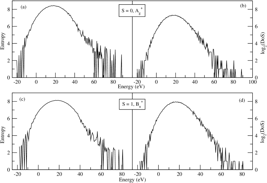
Figure 10: For two spin and spatial symmetry adapted subspaces we compare the entropy profiles with the logarithm of DoS profiles. The system is a 10-site half-filled chain.

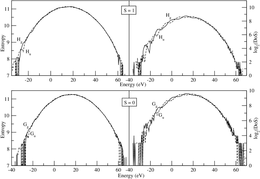
Figure 11: For four spin and spatial symmetry adapted subspaces we compare the entropy profiles with the logarithm of DoS profiles. The system is a 12-site half-filled icosahedron.

4 Conclusion

To summarize, we have studied the effect of long-range interactions on the entanglement of strongly correlated systems. We find that the diagonal interactions do not increase the entropy of the states, even if they are long-ranged. The behavior of the entropy in correlated models can be understood from a VB picture of the eigenstates. The even-odd alternation in the entanglement entropy for even/odd block sizes can also be understood based on such a VB picture and was illustrated by analyzing the spin-1 Heisenberg antiferromagnet. We also studied the effects of spin and spacial symmetry on the entropy of states by examining the correlated icosahedral cluster. We showed an interesting similarity between the profiles of the entropy and the corresponding profiles of the logarithm of the DoS.

5 Acknowledgment

S. R. is thankful to the Department of Science and Technology (DST), India for financial support and Professor Steve White for a helpful discussion. D. S. thanks DST, India for support under SR/S2/JCB-44/2010.

References

- [1] N. D. Mermin, Physics Today 38, 38 (1985).
- [2] V. Vedral, Nature 453, 1004 (2008).
- [3] L. Amico, R. Fazio, A. Osterloh, and V. Vedral, Rev. Mod. Phys. 80, 517 (2008).
- [4] U. Schollwöck, Rev. Mod. Phys. 77, 259 (2005).
- [5] M. Srednicki, Phys. Rev. Lett. 71, 666 (1993).
- [6] G. Vidal, J. I. Latorre, E. Rico, and A. Kitaev, Phys. Rev. Lett. 90, 227902 (2003).
- [7] R. Horodecki, P. Horodecki, M. Horodecki, and K. Horodecki, Rev. Mod. Phys. 81, 865 (2009).
- [8] J. Hubbard, Proc. Roy. Soc. A 276, 238 (1963).
- [9] R. Pariser and R. G. Parr, J. Chem. Phys. 21, 767 (1953).
- [10] J. A. Pople, Trans. Faraday Soc. 49, 1375 (1953).
- [11] K. Ohno, Theor. Chim. Acta 2, 219 (1964).
- [12] L. Pauling, J. Chem. Phys. 1, 280 (1933); L. Pauling and G. W. Wheland, ibid, 1, 362 (1933).
- [13] Z. G. Soos and S. Ramasesha, in Valence Bond Theory and Chemical Structure, edited by D. J. Klein and N. Trinajstic (Elsevier, New York, 1990), p. 81; S. Ramasesha, and Z. G. Soos, in Valence Bond Theory, edited by D. L. Cooper, (Elsevier, New York, 2002), chap. 20.
- [14] S. Ramasesha, and Z. G. Soos, Int. J. Quantum Chem. XXV, 1003 (1984).
- [15] S. Sahoo, and S. Ramasesha, Int. J. Quantum Chem., DOI: 10.1002/qua.23097 (2011).
- [16] S. R. Bondeson, and Z. G. Soos, J. Chem. Phys. 71, 3807 (1979).
- [17] S. Sahoo, R. Rajamani, S. Ramasesha and D. Sen Phys. Rev. B 78, 054408 (2008).
- [18] H. Li and F. D. M. Haldane, Phys. Rev. Lett. 101, 010504 (2008).
- [19] This can be understood from Fig. 11, where the DoS is high in the middle parts; also note that there are thousands of states in each subspace; for instance, the dimension of with is 15861 with each state having 5-fold spatial and 3-fold spin degeneracies.