Dynamical System Analysis of Interacting Variable Modified Chaplygin Gas Model in FRW Universe

Abstract

In this work, we have considered interacting dynamical model taking variable modified Chaplygin gas which plays as dark energy coupled to cold dark matter in the flat FRW universe. Since the nature of dark energy and dark matter is still unknown, it is possible to have interaction between them and we choose the interaction term in phenomenologically. We have converted all the equations in the dynamical system of equations by considering the dimensionless parameters and seen the evolution of the corresponding autonomous system. The feasible critical point has been found and for the stability of the dynamical system about the critical point, we linearize the governing equation around the critical point. We found that there exists a stable scaling (attractor) solution at late times of the Universe and found some physical range of $n$ and the interaction parameter $c$. We have shown that for our calculated physical range of the parameters, the Universe explores upto quintessence stage. The deceleration parameter, statefinder parameters, Hubble parameter and the scale factor have been calculated around the critical point. Finally some consequences around the critical point i.e., the distance measurement of the Universe like lookback time, luminosity distance, proper distance, angular diameter distance, comoving volume, distance modulus and probability of intersecting objects have been analyzed before and after the present age of the Universe.

I Introduction

Recent observations of redshift and luminosity of type Ia supernovae Bachall ; Perlmutter1 ; Perlmutter2 ; Riess , WMAP Bennett , Chandra X-ray Observatory Allen etc. indicate that universe is spatially flat and undergoing accelerated expansion. The most important discovery over the last few decays is to search for the existence of dark energy which violates the strong energy condition i.e., $\rho+3p<0$ Sahni1 ; Peebles0 ; Padmanabhan . The mystifying fluid namely dark energy is understood to dominate the 70% of the Universe and have enough negative pressure to drive current acceleration 30% dark matter (cold dark matters plus baryons). There are various candidates to play the role of the dark energy. The most obvious candidate for dark energy is the cosmological constant with the equation of state $p/\rho=-1$. The type of dark energy represented by a scalar field is often called quintessence. Other dark energy candidates are namely tachyonic field Sen , DBI-essence Martin , Chaplygin gas Kamenshchik , phantom, holographic dark energy hessence dark energy Zhang , k-essenece Armendariz-Picon and dilaton dark energy Lu .

Recently the Chaplygin gas, also named quartessence, characterized by an exotic equation of state $p=-B/\rho$ $(B>0)$, was suggested as a candidate of a unified model of dark energy Kamenshchik . The Chaplygin gas behaves as pressureless fluid for small values of the scale factor and for large values of the scale factor as a cosmological constant, tends to accelerate the expansion. The above equation was generalized to the form $p=-B/\rho^{\alpha}$, $0\leq\alpha\leq 1$ Gorini ; Alam ; Bento . Consequently this was modified to $p=A\rho-B/\rho^{\alpha}$, $0\leq\alpha\leq 1,~{}~{}A>0$ which is known as modified Chaplygin gas Benaoum ; Sahni ; Debnath shows a radiation era $(A=1/3)$ when the scale factor $a(t)$ is vanishingly small and a $\Lambda$CDM model when the scale factor $a(t)$ is infinitely large. Variable Chaplygin gas first proposed by Guo and Zhang Guo with equation of state $p=-B/\rho$, where $B$ is a positive function of the cosmological scale factor $`a$’ i.e., $B=B(a)$. This assumption is reasonable since $B(a)$ is related to the scalar potential if we take the Chaplygin gas as a Born-Infeld scalar field Bento2 . Afterward there are some works on variable Chaplygin gas model Sethi ; Guo2 . Further, Debnath Debnath1 introduced variable modified Chaplygin gas (VMCG) for acceleration of the universe. Several interesting features and physical interpretations of VMCG have been shown by several authors Jamil ; Chatto ; Chatto1 ; Xing . The dynamical system analysis of pure and generalized Chaplygin gas model and the nature of critical points have been analyzed for Einstein’s gravity and loop quantum gravity Wu ; Wu1 ; Zhang1 ; Jamil1 ; Jamil2 ; Jamil3 .

In this work, we consider a model of interacting variable modified Chaplygin gas (VMCG) with dark matter in the framework of Einstein gravity. We construct the formalism of autonomous dynamical system of equations for this interacting model. Since the nature of dark energy and dark matter is still unknown, it is possible to have interaction between them and we choose the interaction term in phenomenologically. We convert them to dimensionless form and perform stability analysis and solve them numerically. We obtain a stable scaling solution (which is also an ‘attractor’) of the equations in FRW model. Some consequences like lookback time, proper distance, luminosity distance, angular diameter distance, comoving volume, distance modulus and probability of intersecting objects of the solution around the critical point have been investigated. We discuss our results in the final section.

II Dynamical model of interacting VMCG and Dark matter

We consider a spatially flat universe with VMCG as dark energy and dark matter interacting through an interaction term. Thus the Einstein equations and continuity equation of VMCG and dark matter can be written respectively as (choosing $8\pi G=c=1$)

$$H^{2}=\frac{1}{3}\rho$$ (1)

$$\dot{H}=-\frac{1}{2}\left(p+\rho\right)$$ (2)

and

$$\dot{\rho}+3H(\rho+p)=0$$ (3)

where $\rho=\rho_{vmcg}+\rho_{dm}$ and $p=p_{vmcg}+p_{dm}$ ($p_{dm}$ is very small quantity, somewhere dark matter assumed as pressureless quantity) are the total cosmic energy density and pressure respectively with the subscripts $vmcg$ and $dm$ denote the VMCG and dark matter respectively. Since we consider that the VMCG and dark matter do not conserve separately, so their continuity equations are

$$\dot{\rho}_{vmcg}+3H\left(\rho_{vmcg}+p_{vmcg}\right)=-Q$$ (4)

and

$$\dot{\rho}_{dm}+3H\left(\rho_{dm}+p_{dm}\right)=Q$$ (5)

To obtain a suitable evolution of the Universe an interaction is often assumed such that the decay rate should be proportional to the present value of the Hubble parameter for good fit to the expansion history of the Universe as determined by the Supernovae and CMB data Berger . Here $Q$ is the interaction term which have dimension of density multiplied by Hubble parameter. For suitable choice of $Q$ is $Q=3cH\rho$, $c$ is the coupling parameter denoting the transfer strength. The interaction term can not be trace out from the first principles due to unidentified scenario of both the dark energy and dark matter. If $Q<0$ then energy density of dark energy become negative at sufficiently early times, therefore the second law of thermodynamics can be violated Alcaniz . Thus $Q$ must be positive and small. Also the observational data of 182 Gold type Ia supernova samples, CMB data from the three year WMAP survey and the baryonic acoustic oscillations from the Sloan Digital Sky Survey estimated that the coupling parameter between dark matter and dark energy must be a small positive value (of the order unity), which satisfies the requirement for solving the cosmic coincidence problem and the second law of thermodynamics Feng .

The VMCG equation of state is given by Debnath1

$$p_{vmcg}=A\rho_{vmcg}-\frac{B(a)}{\rho_{vmcg}^{\alpha}},~{}~{}\mbox{ with $A$, $\alpha$ are constants and $0\leq\alpha\leq 1$}$$ (6)

where $B(a)$ is a positive function of the cosmological scale factor $`a$’. Now consider for simplicity, $B(a)=B_{0}a^{-n}$, where $n$ and $B_{0}$ are constants. More precisely the restriction for accelerating universe becomes $0<n\leq 4$ Debnath1 .

The dark matter equation of state is

$$p_{dm}=w_{dm}\rho_{dm},\mbox{ with $w_{dm}$ is a small constant.}$$ (7)

To analyze the dynamical system, we convert the physical parameter into dimensionless form as follows:

$$x=\ln a,~{}~{}u=\Omega_{vmcg}=\frac{\rho_{vmcg}}{3H^{2}}\mbox{~{}~{}and~{}~{}}v=\frac{p_{vmcg}}{3H^{2}}$$ (8)

The equation of state of the VMCG can be expressed as

$$w_{vmcg}(x)=\frac{p_{vmcg}}{\rho_{vmcg}}=\frac{v}{u}$$ (9)

Defining dimensionless density parameters of dark matter $\Omega_{dm}=\frac{\rho_{dm}}{3H^{2}}$ and using the Friedmann equation (1), we obtain

$$\Omega_{dm}=1-\Omega_{vmcg}=1-u$$ (10)

Thus for the flat universe, $u$ must lies in the region $0\leq u\leq 1$, since the energies of VMCG and dark matter can not be negative.

Now we can cast the evolution equations in the following autonomous system of $u$ and $v$ in the form:

$$\frac{du}{dx}=-3c-3\left(u-1\right)\left(uw_{dm}-v\right)~{},$$ (11)

$$\frac{dv}{dx}=\left\{A(1+\alpha)-\alpha\frac{v}{u}\right\}\left\{-3c-3\left(1+\frac{v}{u}\right)u\right\}+n\left(A-\frac{v}{u}\right)u$$

$$+3v\left\{\left(1+\frac{v}{u}\right)u+\left(1+w_{dm}\right)\left(1-u\right)\right\}$$ (12)

II.1 Critical point

The critical points of the above system are the solution of the equations $\frac{du}{dx}=\frac{dv}{dx}=0$. The only feasible critical point is obtained as

$$u_{crit}=\frac{n-3\left(1-c+w_{dm}\right)\left(1+\alpha\right)}{n-3\left(1+w_{dm}\right)\left(1+\alpha\right)}~{}~{},~{}~{}~{}~{}~{}~{}~{}~{}~{}~{}~{}~{}~{}~{}~{}~{}~{}~{}~{}~{}~{}~{}~{}~{}~{}~{}~{}~{}~{}~{}~{}~{}~{}~{}~{}~{}$$ (13)

$$v_{crit}=-\frac{n^{2}-3n\left(2+w_{dm}\right)\left(1+\alpha\right)+9\left(1+w_{dm}+cw_{dm}\right)\left(1+\alpha\right)^{2}}{3\left(1+\alpha\right)\left\{3\left(1+w_{dm}\right)\left(1+\alpha\right)-n\right\}}$$ (14)

Since in a spatially flat universe, the physically meaningful range of $u$ is $0\leq u\leq 1$, hence $0\leq u_{crit}\leq 1$ leads to the condition $0<c\leq\frac{3\left(1+w_{dm}\right)\left(1+\alpha\right)-n}{3\left(1+\alpha\right)}$ along with $n\leq min\{3(1+w_{dm})(1+\alpha),4\}$, Debnath1 for existence of the critical point. This condition of $c$ represents there is an energy transfer from to dark matter to VMCG.

II.2 Stability around critical point

For the stability of the dynamical system about the critical point, we linearize the governing equation around the critical point i.e., $u=u_{crit}+\delta u$ and $v=v_{crit}+\delta v$, we obtain

$$\delta\left(\frac{du}{dx}\right)=\left[3\left(v+w_{dm}-2uw_{dm}\right)\right]_{crit}\delta u+\left[3\left(-1+u\right)\right]_{crit}\delta v,$$ (15)

$$\delta\left(\frac{dv}{dx}\right)=\left[-3w_{dm}v-\frac{3v(c+v)\alpha}{u^{2}}+A\{n-3(1+\alpha)\}\right]_{crit}\delta u+$$

$$\left[\{3-3A-n+6v+3(1-u)w_{dm}\}+\frac{3(c+u-Au+2v)\alpha}{u}\right]_{crit}\delta v$$ (16)

We find the eigen values of the Jacobian matrix at the critical point (for simplicity we set $\alpha=1$) as in the following:

$$\lambda_{1,2}=\frac{1}{4}\left[3n-6(3+2A+c+w_{dm})+\frac{36c^{2}}{6c+n-6(1+w_{dm})}\right]\pm~{}~{}~{}~{}$$

$$\frac{1}{4}\sqrt{\frac{\left\{(6-n)^{2}+72cw_{dm}-36w_{dm}^{2}+12A\left(6-6c-n+6w_{dm}\right)\right\}}{\{6c+n-6(1+w_{dm})\}}}\times$$

$$\sqrt{\frac{\left\{-144c^{2}+(6-n)^{2}+12A\left(6-6c-n+6w_{dm}\right)-36w_{dm}^{2}-24c\left(n-6-9w_{dm}\right)\right\}}{\{6c+n-6(1+w_{dm})\}}}$$ (17)

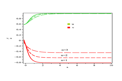
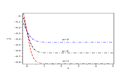
FIG.1                                                                    FIG.2

Figure 1: The dimensionless parameters are plotted against e-folding time for different values of $n$. The initial condition is $v(0)=-0.16,u(0)=0.6$. Other parameters are fixed at $c=0.01,A=0.3$, $w_{dm}=0.01$ and $\alpha$ = 0.8.

Figure 2: The evolution of $w(x)=v/u$ for the interacting VMCG model, corresponding to the initial conditions $u(0)=0.6$, $v(0)=-0.016$; The figure is drawn for different values of $n$, other parameters are fixed at $c=0.01,A=0.3$, $w_{dm}=0.01$ and $\alpha$ = 0.8 respectively.

If the real parts of the above eigenvalues are negative, the critical point is stable node and is a stationary attractor solution; otherwise unstable and thus oscillatory. Physical meaningful range of $c$ is $0\leq c\leq\frac{3\left(1+w_{dm}\right)\left(1+\alpha\right)-n}{3\left(1+\alpha\right)}$ and in this range the critical point $(u_{crit},v_{crit})$ is stable and is a late-time stationary attractor solution. Here we plot some figures to show the properties of evolution of the Universe controlled by the dynamical system (11) and (12). The dimensionless parameters $u$ and $v$ have been drawn in figure 1 in terms of $x=\ln a$. Also the EOS parameter $w_{vmcg}=\frac{v}{u}$ is drawn in figure 2 for $n=1,2,3$. We see that $u$ becomes positive but $v$ and $\frac{v}{u}$ explore to the negative level above $-1$. The phase-space diagrams have been shown in figures 3 and 4 for $n=1,3$ respectively. We see that from the progressions of the phase-portrait, $u$ goes to $1$ and $v$ tends to a negative value above $-1$ and hence the solution is stationary attractor and thee corresponding critical point is a stable node.

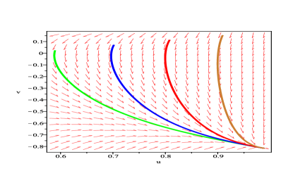
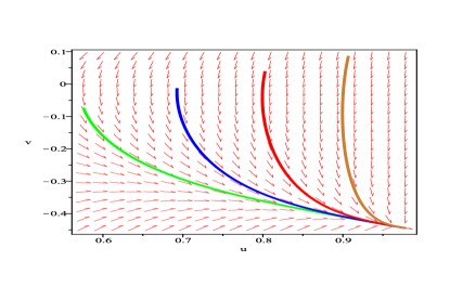
FIG.3                                                                    FIG.4

Figure 3: The phase space diagram of parameters depicting an attractor solution. The initial conditions chosen are $v(0)=-0.16$, $u(0)=0.6$ (green); $v(0)=-0.12$, $u(0)=0.6$ (blue); $v(0)=-0.08$, $u(0)=0.7$ (red); $v(0)=-0.4$, $u(0)=0.8$ (brown). Other parameters are fixed at $c=0.01$, $A=0.3$, $w_{dm}=0.01$, $\alpha=0.8$, $n=1$.

Figure 4: The phase space diagram of parameters depicting an attractor solution. The initial conditions chosen are $v(0)=-0.16$, $u(0)=0.6$ (green); $v(0)=-0.12$, $u(0)=0.6$ (blue); $v(0)=-0.08$, $u(0)=0.7$ (red); $v(0)=-0.4$, $u(0)=0.8$ (brown). Other parameters are fixed at $c=0.01$, $A=0.3$, $w_{dm}=0.01$, $\alpha=0.8$, $n=3$.

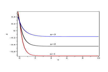
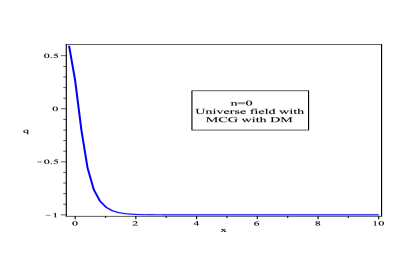
FIG.5                                                                    FIG.6

Figure 5: The deceleration parameter $q$ is plotted against the evolution of the universe for different values of $n$. Other parameters are fixed at $c=0.01$, $A=0.3$, $w_{dm}=0.01$, and $\alpha=0.8$.

Figure 6: The deceleration parameter $q$ is plotted against the evolution of the universe for $n=0$. Other parameters are fixed at $c=0.01$, $A=0.3$, $w_{dm}=0.01$, and $\alpha=0.8$.

At the critical point, the deceleration parameter $q=-1-\left(\dot{H}/H^{2}\right)$ is obtained as

$$q=-1+\frac{3}{2}X,~{}~{}~{}~{}X=1+v_{crit}+w_{dm}(1-u_{crit})$$ (18)

Integrating, we have the Hubble parameter as (ignoring the integrating constant)

$$H=\frac{2}{3Xt}$$ (19)

Again integrating $(19)$, we get

$$a(t)=a_{0}\left(\frac{t}{t_{0}}\right)^{\frac{2}{3X}}$$ (20)

which gives power law expansion of the universe, $a_{0}$ is the present value of the scale factor when $t=t_{0}$ is the present time which is given by $t_{0}=\frac{2}{3XH_{0}}$. Since we have obtained the deceleration parameter $q$, Hubble parameter $H$ and scale factor $a(t)$ around the critical point, so these are valid for the late stage of the evolution of the universe i.e., when time $t$ is very large. Thus $X$ should be taken positive value for positivity of the Hubble parameter $H$ and hence the scale factor $a(t)$ is increasing function of time $t$. So from (18), we obtain $q\in(-1,0)$ for accelerating phase of the universe if $X\in(0,2/3)$. So the VMCG couples with dark matter filled in the universe always drives acceleration. Figure 5 shows the graph of $q$ against $x=\ln a$ for some particular values of $n=1,2,3$. For $n=0$, the VMCG model reduces to MCG and these couples with dark matter filled in the universe always drives acceleration and this model explores upto $\Lambda$CDM stage ($q=-1$) (figure 6).

II.3 Statefinder parameters

We also determine the dimensionless pair of cosmological diagnostic pair $\{r,s\}$ dubbed as statefinder parameters introduced by Sahni et al Sahni . The two parameters have a great geometrical significance since they are derived from the cosmic scale factor alone, though one can rewrite them in terms of the parameters of dark energy and matter. Furthermore, the pair characterize the properties of dark energy in a model-independent manner i.e. independent on the theory of gravity. Also this pair generalizes the well known geometrical parameters like the Hubble parameter and the deceleration parameter. The parameter $r$ forms the next step in the hierarchy of geometrical cosmological parameters $H$ and $q$. The parameters are given by

$$r\equiv\frac{\dddot{a}}{aH^{3}}=\left(1-\frac{3X}{2}\right)\left(1-3X\right),~{}~{}~{}~{}s\equiv\frac{r-1}{3(q-1/2)}=X$$ (21)

where $X$ is obtained in equation (18). Since we have already obtained that for accelerating universe, $X<2/3$. In this range, $s$ is always positive. But $r>0$ for $X<1/3$ and $r<0$ for $1/3<X<2/3$.

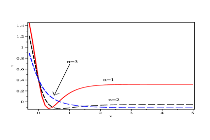
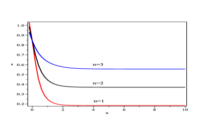
FIG.7                                                                    FIG.8

Figure 7: The statefinder parameter $r$ is plotted against the evolution of the universe for different values of $n$. Other parameters are fixed at $c=0.01$, $A=0.3$, $w_{dm}=0.01$, and $\alpha=0.8$.

Figure 8: The statefinder parameter $s$ is plotted against the evolution of the universe for different values of $n$. Other parameters are fixed at $c=0.01$, $A=0.3$, $w_{dm}=0.01$, and $\alpha=0.8$.

III Consequences: Distance Measurement of the Universe

In cosmography (the measurement of the Universe) there are many ways to specify the distance between two points, because in the expanding and accelerating Universe, the distances between comoving objects are constantly changing, and Earth-bound observers look back in time as they look out in distance. The unifying aspect is that all distance measures somehow measure the separation between events on radial null trajectories, i.e., trajectories of photons which terminate at the observer. Here we will compute various cosmological distance measures. In this section, we shall discuss the lookback time, luminosity distance, proper distance, angular diameter distance, comoving volume, distance modulus and probability of intersecting objects.

III.1 Lookback Time

The lookback time to an object is the difference between the age of the Universe now (at observation) and the age of the Universe at the time the photons were emitted (according to the object). As light travels with finite speed, it takes time for it to cover the distance related to the redshift it encountered. So, a look into space is always a look back in time. It is used to predict properties of high redshift objects with evolutionary models, such as passive stellar evolution for galaxies. Thus if a photon emitted by a source at the instant $t$ and received at the time $t_{0}$ then the photon travel time or the lookback time $t_{0}-t$ is defined by Debnath2 ; Arbab ; Hogg ; Peebles ; Kolb

$$t-t_{0}=\int^{a}_{a_{0}}{\frac{da}{\dot{a}}}$$ (22)

where $a_{0}$ is the present value of the scale factor of the universe and can be obtained from (20) at $t=t_{0}$. The redshift is an important observable as they can be measured easily from the spectral lines and the redshift increases of an object with its distance from us. Lookback time is used to predict properties of high-redshift objects with evolutionary models, such as passive stellar evolution for galaxies. The redshift $z$ can be defined by

$$\frac{a_{0}}{a}=1+z=\left(\frac{t_{0}}{t}\right)^{\frac{2}{3X}}$$ (23)

which gives the lookback time in the following form

$$t-t_{0}=\frac{2}{3XH_{0}}\left\{\frac{1}{\left(1+z\right)^{\frac{3X}{2}}}-1\right\}$$ (24)

For accelerating universe we have already get $X<\frac{2}{3}$. Early universe is represented by $z\rightarrow\infty$ implies $t\rightarrow 0$ and late universe $z\rightarrow-1$, which equivalently implied $t\rightarrow\infty$. Also $z\rightarrow 0$ gives the present age $t\rightarrow t_{0}$ of the universe.

III.2 Proper Distance

As light needs time to get from an object to the observer, one can define a distance that may be measured between the observer and the object with a ruler at the time the light was emitted, the proper distance. When a photon emitted by a source and received by an observer at time $t_{0}$ then the proper distance between them is defined by Debnath2 ; Arbab ; Hogg ; Peebles ; Weinberg ; Weedman

$$d=a_{0}\int^{a_{0}}_{a}{\frac{da}{a\dot{a}}}=a_{0}\int^{t_{0}}_{t}{\frac{dt}{a}}$$ (25)

which gives

$$d=\frac{2}{H_{0}(3X-2)}\left\{1-\frac{1}{\left(1+z\right)^{\frac{3X}{2}-1}}\right\}$$ (26)

The proper distance may also called the comoving distance (line of sight) of the Universe in today. So between two nearby objects in the Universe, the distance between them which remains constant with epoch if the two objects are moving with the Hubble flow. In other words, it is the distance between them which would be measured with rulers at the time they are being observed divided by the ratio of the scale factor of the Universe then to now. Next thing to be defined is the transverse comoving distance, which is a quantity used to get the comoving distance perpendicular to the line of sight. For flat universe, the transverse comoving distance is always identical to the comoving distance (line of sight). That means the transverse comoving distance $=$ proper distance $=d$, for our model of the flat FRW Universe.

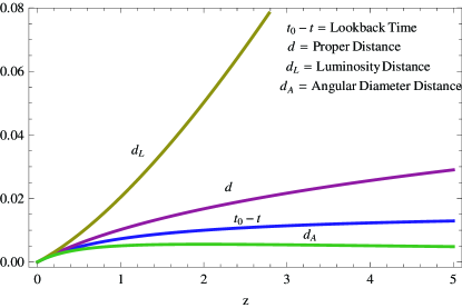
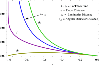
FIG.9                                                                    FIG.10

Figure 9: Look back time, proper distance, luminosity distance and angular diameter distance as a function of redshift assuming $H_{0}=72km/s/Mpc$ before the present age of the universe.

Figure 10: Look back time, proper distance, luminosity distance and angular diameter distance as a function of redshift assuming $H_{0}=72km/s/Mpc$ after the present age of the universe.

III.3 Luminosity Distance

If $L$ be the total energy emitted by the source per unit time and $\ell$ be the apparent luminosity of the object then the luminosity distance is defined by Debnath2 ; Arbab ; Hogg ; Weinberg ; Weedman

$$d_{L}=\left(\frac{L}{4\pi\ell}\right)^{\frac{1}{2}}=d(1+z)=\frac{2}{H_{0}(3X-2)}\left\{(1+z)-\frac{1}{(1+z)^{\frac{3X}{2}}}\right\}$$ (27)

III.4 Angular Diameter Distance

The angular diameter of a light source of proper distance $D$ observed at $t_{0}$ is defined by Debnath2 ; Arbab ; Hogg ; Peebles ; Weinberg ; Weedman

$$\delta=\frac{D(1+z)^{2}}{d_{L}}$$ (28)

The angular diameter distance $(d_{A})$ is defined as the ratio of the source diameter to its angular diameter (in radians) as

$$d_{A}=\frac{D}{\delta}=d_{L}(1+z)^{-2}=d(1+z)^{-1}$$ (29)

For our model angular diameter distance $(d_{A})$ is given by,

$$d_{A}=\frac{2}{H_{0}(3X-2)}\left\{\frac{1}{1+z}-\frac{1}{\left(1+z\right)^{\frac{3X}{2}-2}}\right\}$$ (30)

It is used to convert angular separations in telescope images into proper separations at the source. It is famous for not increasing indefinitely as $z\rightarrow\infty$; it turns over at $z\sim 1$ and thereafter more distant objects actually appear larger in angular size. The angular diameter distance is maximum at

$$z_{max}=\left(\frac{2}{3X-2}\right)^{\frac{2}{3(2-X)}}-1$$ (31)

and corresponding maximum angular diameter $d_{A}|_{max}$ taking the form

$$d_{A}|_{max}=\frac{1}{H_{0}(3X-2)}\left[2^{1+\frac{2}{3(X-2)}}\left(\frac{1}{3X-4}\right)^{\frac{2}{3(X-2)}}-2\left\{4^{\frac{1}{3(2-X)}}\left(\frac{1}{3X-4}\right)^{\frac{2}{3(X-2)}}\right\}^{2-\frac{3X}{2}}\right]$$ (32)

Look back time, proper distance, luminosity distance and angular diameter distance before and after the present age of the universe are respectively drawn in figures 9 and 10.

III.5 Comoving Volume

The comoving volume $V_{C}$ is the volume measure in which number densities of non-evolving objects locked into Hubble flow are constant with redshift as Hogg ; Peebles ; Weinberg

$$dV_{C}=D_{H}\frac{(1+z)^{2}d_{A}}{E(z)}d\Omega dz=\frac{1}{H_{0}}(1+z)^{2-\frac{3X}{2}}d_{A}^{2}d\Omega dz$$ (33)

where $d\Omega$ is the solid angle element and $d_{A}$ is the angular diameter, $E(z)=\frac{H(z)}{H_{0}}$ and $D_{H}=\frac{c}{H_{0}}$ is the Hubble distance ($c$ is the velocity of light) and in our model we assume $c=1$, $d\Omega=1$, $H_{0}=72km/s/Mpc$. So, the comoving volume is proper volume times the ratio of scale factors now to then to the third power. Comoving volume element $dV_{C}/dz$ before and after the present age of the universe are respectively drawn in figures 11 and 12. We see that when $z>0$, the volume element decreases as $z$ decreases and when $z<0$, the volume element increases as $z$ decreases.

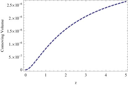
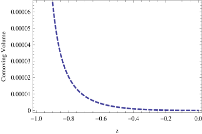
FIG.11                                                                    FIG.12

Figure 11: Comoving volume element $dV_{C}/dz$ as a function of redshift assuming $H_{0}=72km/s/Mpc$, $d\Omega=1$, before the present age of the universe.

Figure 12: Comoving volume element $dV_{C}/dz$ as a function of redshift assuming $H_{0}=72km/s/Mpc$, $d\Omega=1$, after the present age of the universe.

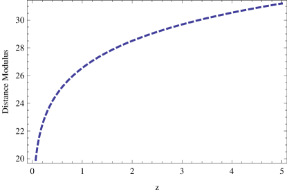
FIG.13                                                                    FIG.14

Figure 13: Distance modulus $D_{M}$ as a function of redshift before the present age of the universe.

Figure 14: Distance modulus $D_{M}$ as a function of redshift after the present age of the universe.

III.6 Distance Modulus

The distance modulus is define by

$$D_{M}=5\log\left(\frac{d_{L}}{10pc}\right)$$ (34)

because it is the magnitude difference between an object s observed bolometric (i.e., integrated over all frequencies) flux and what it would be if it were at 10 pc (this was once thought to be the distance to Vega) and $d_{L}$ is the luminosity distance. Distance modulus $D_{M}$ as a function of redshift before and after the present age of the universe have been shown in figures 13 and 14. We see that for $z>0$, $D_{M}$ decreases as $z$ decreases but for $z<0$, $D_{M}$ increases as $z$ decreases upto a certain stage (about $z\sim-0.6$) and after that $D_{M}$ decreases as $z$ decreases.

III.7 Probability of intersecting objects

The incremental probability $dP$ that a line of sight will intersect one of the objects in redshift interval $dz$ at redshift $z$ is given by Hogg ; Peebles

$$dP=n(z)\sigma(z)D_{H}\frac{(1+z)^{2}}{E(z)}dz$$ (35)

where $n(z)$ is the comoving number density and $\sigma(z)$ areal cross-section. Assuming $n(z)\sigma(z)=1$, we obtain

$$dP=\frac{1}{H_{0}}(1+z)^{2-\frac{3X}{2}}dz$$ (36)

For our model the expression of Probability of intersecting objects becomes

$$P=\frac{2}{H_{0}(6-3X)}\left\{(1+z)^{3-\frac{3X}{2}}-1\right\}$$ (37)

In figures 15 and 16 we draw intersection probability $P$ as a function of redshift before and after the present age of the universe respectively. We see that for $z>0$, $P$ decreases as $z$ decreases and for $z<0$, $P$ increases as $z$ decreases.

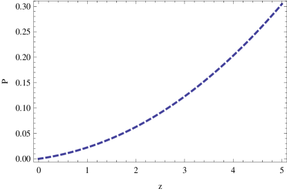
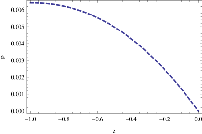
FIG.15                                                                    FIG.16

Figure 15: Intersection probability $P$ as a function of redshift before the present age of the universe.

Figure 16: Intersection probability $P$ as a function of redshift after the present age of the universe.

IV Discussions

In this work, we have considered flat FRW model of the universe in Cosmology. We have assumed that the dark energy can be considered in the form of variable modified Chaplygin gas (VMCG). The interaction between dark matter and VMCG has been investigated in this model. To analyze the dynamical system, we have converted the physical parameters into dimensionless form. We have made a comprehensive phase-plane analysis for the VMCG model. Our main aim was to investigate the properties of critical point of the dynamical system which play crucially important roles for this interacting model. We have found only one critical point which is physically justified. Next we consider small fluctuation about the critical point $(u_{crit},v_{crit})$ and found the eigen values of the corresponding Jacobian matrix for $\alpha=1$. It has been observed that the all eigen values are negative for all physical choices of parameters and a stable attractor scaling solution is obtained.

In figure $1$, we plot dimensionless parameters $u$ and $v$ with respect to $x=\ln a$. We notice that $u$ converges toward $u=1$ in the region $0<n<4$ (in particular, for $n=1,2,3$), also $v$ decreases simultaneously and keeps negative sign in near future. This signifies the dark energy dominating nature of the universe which means the energy flows from all dark matter to dark energy. Also if we change the values of $\alpha$, then it may be seen that nature of the dimensionless quantities $u$ and $v$ do not sensitively depend on the change of $\alpha$. Figure 2 depicts that the ratio $v/u=w_{vmcg}$ gets the same nature with the variation of $n$. Since in a spatially flat universe, the physically meaningful range of $u_{crit}$ is $0\leq u_{crit}\leq 1$ leads to the condition $0<c\leq\frac{3\left(1+w_{dm}\right)\left(1+\alpha\right)-n}{3\left(1+\alpha\right)}$ along with $n\leq min\{3(1+w_{dm})(1+\alpha),4\}$, for existence of the critical point. This condition of $c$ represents there is an energy transfer from to dark matter to VMCG. The phase diagram in $u$-$v$ space (figures 3,4) shows the attractor solution for $n=1,3$. In the above range, the critical point $(u_{crit},v_{crit})$ is stable. Thus the present state and the future evolution do not depend sensitively on the choice of the initial condition. Our model cannot cross phantom divide, which is consistent with the previous work Debnath1 , since we have chosen power law form of $B(a)$. If we choose another form of $B(a)$, then the VMCG model may cross the phantom barrier, which is more difficult than this one. We may consider this type of problem in near future.

Moreover the expansion of the universe is governed by a power law form around the critical point. Hence the expansion will go on forever with an ever increasing rate. We have also studied the evolution of the deceleration parameter $q(x)=-\frac{\ddot{a}}{a\dot{a}^{2}}=-1+\frac{3}{2}\left(1+v(x)+w_{dm}(1-u(x))\right)$ for the interacting VMCG model with dark matter. The result is shown in figure 5 with different parameters value ranging from $n=1$ to $n=3$. Therefore, one can observed that for $n=1,2,3$ the values of $q$ decrease from positive value to negative value but cannot reached $-1$. On the other way, figure 6 shows that $q$ decreases from positive value to $-1$ for $n=0$. So VMCG ($n\neq 0$) generates quiessence scenario for late stage but only MCG ($n=0$) generates the $\Lambda$CDM model for late stage of the Universe. Also we have obtained the statefinder parameters at the critical point. Around the critical point, the natures of the parameters are drawn in figures 7 and 8. In all the above figures, we have chosen $c=0.01,A=0.3,w_{dm}=0.01$ and $\alpha=0.8$.

Distance measurements of the Universe around the critical point have been discussed. The look back time, proper distance, luminosity distance, angular diameter distance, comoving volume, distance modulus and probability of intersecting objects before and after the present age of the universe have been calculated in terms of $z$, $X$ and $H_{0}$ and their progressions are shown in figures 9 -16. For all figures, we have assumed $H_{0}=72km/s/Mpc$. The maximum angular diameter distance has been found for a particular value of redshift $z$. Comoving volume element $dV_{C}/dz$ before and after the present age of the universe are respectively drawn in figures 11 and 12. We see that when $z>0$, the volume element decreases as $z$ decreases and when $z<0$, the volume element increases as $z$ decreases. Distance modulus $D_{M}$ as a function of redshift before and after the present age of the universe have been shown in figures 13 and 14. We see that for $z>0$, $D_{M}$ decreases as $z$ decreases but for $z<0$, $D_{M}$ increases as $z$ decreases upto a certain stage (about $z\sim-0.6$) and after that $D_{M}$ decreases as $z$ decreases. In figures 15 and 16 we draw intersection probability $P$ as a function of redshift before and after the present age of the universe respectively. We see that for $z>0$, $P$ decreases as $z$ decreases and for $z<0$, $P$ increases as $z$ decreases. So these are the main consequences of the power law form of scale factor.

Acknowledgement:

One of the authors (JB) is thankful to CSIR, Govt of India for providing Junior Research Fellowship.

References

- (1) N. A. Bachall, J. P. Ostriker, S. Perlmutter and P. J. Steinhardt, Science 284 1481 (1999).
- (2) S. J. Perlmutter et al, Bull. Am. Astron. Soc. 29, 1351 (1997).
- (3) S. J. Perlmutter et al, Astrophys. J. 517 565 (1999).
- (4) A. G. Riess et al, Astron. J. 116, 1009 (1998).
- (5) C. L. Bennett et al, Astrophys. J. Suppl. 148, 1 (2003).
- (6) S. W. Allen et al, Mon. Not. Roy. Astron. Soc. 353, 457 (2004).
- (7) V. Sahni and A. A. Starobinsky, Int. J. Mod. Phys. A 9, 373 (2000).
- (8) P. J. E. Peebles and B. Ratra, Rev. Mod. Phys. 75, 559 (2003).
- (9) T. Padmanabhan, Phys. Rept. 380, 235 (2003).
- (10) A. Sen, JHEP 065 0207 (2002).
- (11) J. Martin and M. Yamaguchi, Phys. Rev. D 77 103508 (2008).
- (12) A. Kamenshchik et al, Phys. Lett. B 511 265 (2001).
- (13) H. Wei, R. G. Cai and D. F. Zhang, Class. Quantum Grav. 22 3189 (2005).
- (14) C. Armendariz-Picon et al, Phys. Rev. D 63 103510 (2001).
- (15) H. Q. Lu et al, hep-th/0409309.
- (16) V. Gorini, A. Kamenshchik and U. Moschella, Phys. Rev. D 67, 063509 (2003).
- (17) U. Alam, V. Sahni, T. D. Saini and A. A. Starobinsky, Mon. Not. R. Astron. Soc. 344, 1057 (2003).
- (18) M. C. Bento, O. Bertolami and A. A. Sen, Phys. Rev. D 66, 043507 (2002).
- (19) H. B. Benaoum, hep-th/0205140.
- (20) U. Debnath, A. Banerjee and S. Chakraborty, Class. Quantum Grav. 21, 5609 (2004).
- (21) V. Sahni, T. D. Saini, A. A. Starobinsky and U. Alam, JETP Lett. 77, 201 (2003).
- (22) Z.K. Guo, Y.Z. Zhang, Phys. Lett. B 645, 326 (2007).
- (23) M.C. Bento, O. Bertolami, A.A. Sen Phys. Lett. B 575, 172 (2003).
- (24) Z.K. Guo, Y.Z. Zhang, astro-ph/0509790.
- (25) G. Sethi, S.K. Singh, P. Kumar, D. Jain and A. Dev, Int. J. Mod. Phys. D 15, 1089 (2006).
- (26) U. Debnath, Astrophys. Space Sci. 312, 295 (2007).
- (27) M. Jamil and M. A. Rashid, Eur. Phys. J. C 58, 111 (2008).
- (28) S. Chattopadhyay and U. Debnath, Grav. Cosmol. 14, 341 (2008).
- (29) S. Chattopadhyay and U. Debnath, Astrophys. Space Sci. 319, 183 (2009).
- (30) L. Xing, Y. Gui, L. Xu and J. Lu, Mod. Phys. Lett. A 24, 683 (2009).
- (31) P. Wu and H. Yu, Class. Quantum Grav. 24, 4661 (2007).
- (32) P. Wu and S. N. Zhang, JCAP 0806, 007 (2008).
- (33) H. Zhang and Z. -H. Zhu, Phys. Rev. D 73 043518 (2006).
- (34) M. Jamil and M. A. Rashid, Eur. Phys. J. C 60, 141 (2009).
- (35) M. Jamil, Int. J. Theor. Phys. 49, 62 (2010).
- (36) M. Jamil and U. Debnath, Astrophys. Space Sci. 333, 3 (2011).
- (37) M. S. Berger and H. Shojaei, Phys. Rev. D 74, 043530 (2006).
- (38) J. S. Alcaniz and J. A. S. Lima, Phys. Rev. D 72, 063516 (2005).
- (39) C. Feng, et al, Phys. Lett. B 665, 111 (2008).
- (40) M. Jamil and U. Debnath, Int. J. Theor. Phys. 50, 1602 (2011).
- (41) A. I. Arbab, astro-ph/9810239.
- (42) D. W. Hogg, astro-ph/9905116v4.
- (43) P. J. E. Peebles, Principles of Physical Cosmology, Princeton University Press, Princeton (1993).
- (44) E. W. Kolb and M. S. Turner, The Early Universe, Addison-Wesley, Redwood City (1990).
- (45) S. Weinberg, Gravitation and Cosmolgy: Principles and Applications of the General Theory of Relativity, John Wiley & Sons, New York (1972).
- (46) D. W. Weedman, Quasar Astronomy, Cambridge University, Cambridge (1986).