• Application of a Bayesian Method to Absorption Spectral-Line Finding in Simulated ASKAP Data

  J. R. Allison^A,D, E. M. Sadler^A,B, and M. T. Whiting^{C
  A} Sydney Institute for Astronomy, School of Physics A28, University of Sydney, NSW 2006, Australia
  ^B ARC Centre of Excellence for All-sky Astrophysics (CAASTRO)
  ^C CSIRO Astronomy & Space Science, P.O. Box 76, Epping NSW 1710, Australia
  ^D Corresponding author. Email: jra@physics.usyd.edu.au

  Abstract: The large spectral bandwidth and wide field of view of the Australian SKA Pathfinder radio telescope will open up a completely new parameter space for large extragalactic HI surveys. Here we focus on identifying and parametrising HI absorption lines which occur in the line of sight towards strong radio continuum sources. We have developed a method for simultaneously finding and fitting HI absorption lines in radio data by using multi-nested sampling, a Bayesian Monte Carlo algorithm. The method is tested on a simulated ASKAP data cube, and is shown to be reliable at detecting absorption lines in low signal-to-noise data without the need to smooth or alter the data. Estimation of the local Bayesian evidence statistic provides a quantitative criterion for assigning significance to a detection and selecting between competing analytical line-profile models.

  Keywords: methods: data analysis — methods: statistical — radio lines: galaxies

1 Introduction

The Australian Square Kilometre Array Pathfinder’s (ASKAP; Deboer et al. 2009) large spectral bandwidth and wide field of view will dramatically improve our ability to conduct large-area galaxy surveys in the 21 cm line of neutral hydrogen (Johnston et al. 2007).

The ASKAP HI All-Sky Survey (WALLABY Science Survey Proposal; Koribalski & Staveley-Smith 2009) will cover 75 of the sky ($-90\,\mathrm{deg}<\mathrm{Dec.}<+30\,\mathrm{deg}$) at a spatial resolution of approximately 30 arcsec and velocity resolution of approximately 4 km s^-1. With an integration time of 8 h per pointing (assuming a system temperature of 50 K) the survey will allow us to examine the HI properties and large-scale distribution of $\sim$500,000 galaxies out to a redshift of 0.26 (equivalent to a look-back time of approximately 3 Gyr).

ASKAP will also be a powerful instrument for carrying out blind HI absorption-line surveys using background radio continuum sources. The advantage of absorption-line surveys is that their sensitivity depends only on the brightness of the background source, making it possible to probe the neutral gas content of individual galaxies at redshifts where the HI emission line is too weak to be detectable.

The ASKAP First Large Absorption Survey in HI (FLASH Science Survey Proposal; Sadler et al. 2009) will search for HI and OH absorption features in two redshift ranges ($0<z<0.26$ and $0.5<z<1.0$) using bright background continuum sources from the existing SUMSS (Mauch et al. 2003) and NVSS (Condon et al. 1998) catalogues, both of which have an angular resolution of 45 arcsec. This amounts to a targeted search of over 150,000 sightlines to background continuum sources, an increase of more than two orders of magnitude over the total number of sightlines probed in all previous HI absorption-line surveys with radio telescopes. In the lower ($0<z<0.26$) redshift range, the same ASKAP data are used for the FLASH and WALLABY surveys, making it possible to cross-compare emission- and absorption-line measurements of local galaxies.

FLASH will search all ASKAP HI data cubes for absorption lines at the positions of radio continuum sources with flux densities above 50 mJy in the 1.4 GHz NVSS and 843 MHz SUMSS surveys. Since the positions of these background continuum sources are already known, the ‘source-finding problem’ for FLASH is reduced to the need for a reliable ‘line-finding’ algorithm which can be efficiently applied at a large number of pre-determined positions on the sky. When characterising the detected lines, we want to obtain a reliable analytical model of the line profile and distinguish between competing models, even in the low signal-to-noise (SNR) regime.

A robust quantitative method of selecting between competing models, and measuring the significance of a detection, is provided through the calculation of the Bayesian evidence statistic. This method is already being used for a range of other low SNR astrophysical scenarios, including model fitting to observations of the Sunyaev-Zel’dovich Effect (see e.g. Marshall et al. 2003; Feroz et al. 2009; Allison et al. 2011), where we are interested in comparing between competing models for a redshift-independent observable.

In this paper we present the application of an existing Bayesian Monte Carlo algorithm to the problem of assigning significance to the detection and modeling of HI absorption lines in a simulated ASKAP data cube. Unless otherwise stated, all errors refer to the 68.3 % interval.

2 Simulated data

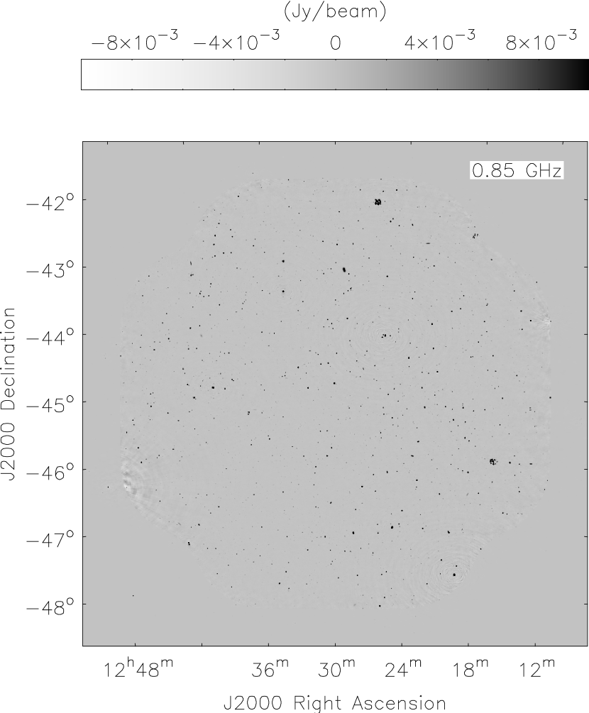
The expected properties of a full ASKAP data cube include a 30 deg² field of view and 300 MHz of bandwidth with 16,384 channels, corresponding to an HI velocity resolution of 12 km s^-1 at 800 MHz. Present computing limitations meant that it was only possible to simulate 1024 spectral channels over the full 30 deg² ASKAP field, equating to 18 MHz of spectral bandwidth. A simulated ASKAP–FLASH data cube covering the redshift range $0.76<z<0.792$ was released by the ASKAP computing group in May 2011, and details were made publically available online.

The FLASH simulation included both spectral-line and continuum information, and the basic steps were:

1. Create a realistic continuum sky simulation at 850 MHz, using the semi-empirical SKADS simulation by Wilman et al. (2008) and an assumed integration time of two hours per pointing (see Figure 1).

2. ‘Paint in’ a grid of Gaussian HI absorption-line profiles covering a range in velocity full width at half maximum (FWHM) and peak optical depth $\tau$. S/N calculations indicate that only sources stronger than about 50 mJy beam^-1 are realistic targets for the FLASH survey (with a planned observing time of two hours per ASKAP pointing), but sources with flux densities down to 10 mJy beam^-1 had HI absorption lines added in the simulation so that our line-finding method could be tested in the low S/N regime.

To provide a useful test of line-finding algorithms, the number of absorption lines inserted into the simulated data is far higher than the number that we would expect to see in a real ASKAP data cube. In total 600 lines (each with a single Gaussian profile) were inserted into the simulated cube. They spanned a redshift range $0.76<z<0.792$, with optical depths $0.01<\tau<0.30$ and velocity widths between 5 and 80 km s^-1. Not all of these lines are expected to be detectable in the final simulated data cube.

The continuum and spectral-line datasets were kept separate to mimic the effects of continuum subtraction, since the capability to do this in the ASKAP pipeline had not yet been fully implemented.

Figure 1: Top: A simulated 850MHz continuum ASKAP image based on the semi-empirical SKADS simulation by Wilman et al. (2008). The maximum pixel value has been limited to 0.01 Jy beam^-1 to prevent the brightest sources from dominating the image. Bottom: An example continuum-subtracted spectrum extracted from the ASKAP–FLASH simulated data cube at the position, $\mathrm{RA(J2000)}=12^{\mathrm{h}}28^{\mathrm{m}}26\hbox{$.\!\!^{{\mathrm{s}}}$}86$ and $\mathrm{Dec.(J2000)}=-47{\hbox{${}^{\circ}$}}03{\hbox{${}^{\prime}$}}31{\hbox{$.\!\!^{\prime\prime}$}}50$, of a source of flux density $S_{800}$ = 198.7 mJy. The red lines indicate the positions of two HI absorption-line components present in the spectrum. Component a is clearly visible above the noise level.

3 Method

To search for HI absorption from neutral gas in distant galaxies we target sightlines towards known bright continuum sources, since the detection probability for an HI absorption line is independent of redshift but increases with the brightness of the background continuum source. The blind aspect of the survey arises from searching for absorption dips in the spectral domain, so we do not need a 3-dimensional source finder, such as Duchamp (Whiting 2008, Whiting et al. in prep.). Instead, we need a tool that detects any spectral lines, quantifies their properties based on an analytical model, and provides an estimate of the detection significance. Standard $\chi^{2}$ minimisation and residual inspection have previously been used to fit parametrised Gaussian models in HI absorption surveys (see e.g. Gupta et al. 2010; Kanekar et al. 2009), and the analysis outlined in this work uses a generalised extension of those methods. In the following sections we discuss a Bayesian approach to the one-dimensional line-finding problem.

3.1 Spectra extraction

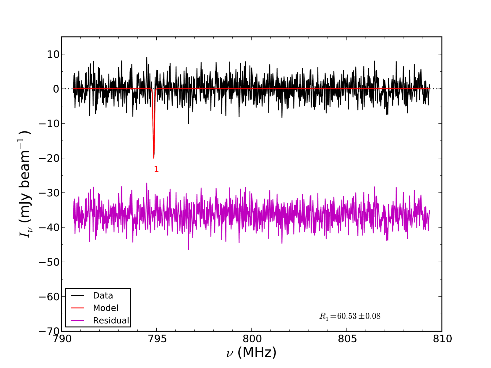
One-dimensional spectra are extracted from the simulated ASKAP data cube using a scripted Python routine in the Casa data reduction package. An input catalogue of the 435 continuum sources that contain simulated HI absorption lines is used to provide the known positions from which the spectra are extracted. Extraction is performed at the centre position of each source using the task Imval in Casa. Each source is indexed based on its flux density at $800\,$MHz, ordered in descending value. Figure 1 shows an example of an extracted spectrum from a continuum source, in which there are two HI absorption-line components. One of the components is clearly visible by eye at 794.9 MHz ($z=0.787$), while the other is buried within the noise at 807.0 MHz ($z=0.760$). The spectral data are stored as individual data files for each continuum source with information on the frequency, brightness and uncertainty. The uncertainties in the data are estimated based on the median of the absolute deviations from the median value (MADFM). This statistic is a more robust estimator of the true uncertainty than the RMS when a strong signal is present in the data. For Gaussian distributed data, the true standard deviation is estimated by multiplying the MADFM statistic by a factor of 1.4826042. The spectra are also stored in Flexible Image Transport System (FITS, Wells et al. 1981) format, so that they are compatible for use with the Duchamp source finder.

Figure 2: Top: Example of spectral-line fitting to a simulated ASKAP source ($\mathrm{RA}=12^{\mathrm{h}}28^{\mathrm{m}}26\hbox{$.\!\!^{{\mathrm{s}}}$}86$, $\mathrm{Dec.}=-47{\hbox{${}^{\circ}$}}03{\hbox{${}^{\prime}$}}31{\hbox{$.\!\!^{\prime\prime}$}}50$, $S_{800}$ = 198.7 mJy). One of the absorption-line components is detected , while the other is hidden in the simulated noise. The residual has been plotted with an offset from the frequency axis for clarity. Bottom: Estimate of the marginialised posterior probabilities for absorption-line parameters from the example detected source. The parameters displayed are the peak optical depth ($\tau$), redshift ($z$) and velocity FWHM ($\Delta v$). The grey-scale represents the 68.3, 95.4, and 99.7% intervals. The dashed lines represent the input catalogue values.

3.2 Bayesian inference

We fit analytical models to the extracted spectral data using Bayesian inference. The posterior (or joint) probability for a set of model parameters ($\boldsymbol{\theta}$), given the data ($\boldsymbol{d}$) and the model hypothesis ($\mathcal{M}$), can be calculated from Bayes’ theroem,

$$\mathrm{Pr}(\boldsymbol{\theta}|\boldsymbol{d},\mathcal{M})={\mathrm{Pr}(\boldsymbol{d}|\boldsymbol{\theta},\mathcal{M})\mathrm{Pr}(\boldsymbol{\theta}|\mathcal{M})\over\mathrm{Pr}(\boldsymbol{d}|\mathcal{M})}.$$ (1)

The probability of the data given the model parameters, known as the likelihood, can be calculated based on assumptions about the distribution of the uncertainty in the data. If the data set is large and therefore quasi-continuous (such as the thermal noise generated in radio instrumentation), one can approximate the likelihood by the form given for Gaussian multivariate data (see e.g. Sivia 2006)

$$L \equiv\mathrm{Pr}(\boldsymbol{d}|\boldsymbol{\theta},\mathcal{M})$$

$$={1\over\sqrt{(2\pi)^{N}|\mathbf{C}|}}\exp{\left[-{(\boldsymbol{d}-\boldsymbol{m})^{\mathrm{t}}\mathbf{C}^{-1}(\boldsymbol{d}-\boldsymbol{m})\over 2}\right]},$$ (2)

where $N$ is equal to the size of $\boldsymbol{d}$, $\mathbf{C}$ is the covariance matrix of the data, $|\mathbf{C}|$ is the determinant of the covariance matrix and $\boldsymbol{m}$ is the vector of model data. In the special case where the variance in the data is a constant ($\sigma^{2}$) and uncorrelated, the above expression for the likelihood reduces to

$$L={1\over\sigma^{N}\sqrt{(2\pi)^{N}}}\exp{\left[-{\sum_{\mathrm{i}}(d_{\mathrm{i}}-m_{\mathrm{i}})^{2}\over 2\sigma^{2}}\right]}.$$ (3)

The probability of the parameter values given the model hypothesis, $\mathrm{Pr}(\boldsymbol{\theta}|\mathcal{M})$, is often known as the prior probability and encodes information about the parameter values a priori. For example, consider the situation where the frequency position of an intervening HI absorber has been relatively well constrained from previous observations. If we trust these observations we might then choose to apply a normal prior to the spectral-line position based on the known level of uncertainty. We would otherwise apply uninformative priors to the parameters if we were are previously unaware of their value. Uninformative priors are typically uniform in either linear space (for location parameters) or logarithmic space (for scale parameters, known as Jeffery’s prior).

The normalisation of the posterior probability in Equation 1 is equal to the probability of the data given the model hypothesis and is referred to throughout this work as the evidence. The evidence is calculated by marginalising the product of the likelihood and prior distributions over the model parameters. This is given by

$$E \equiv\mathrm{Pr}(\boldsymbol{d}|\mathcal{M})$$

$$=\int{\mathrm{Pr}(\boldsymbol{d}|\boldsymbol{\theta},\mathcal{M})\mathrm{Pr}(\boldsymbol{\theta}|\mathcal{M})\mathrm{d}\boldsymbol{\theta}},$$ (4)

which follows from the relation given by Equation 1 and that the integrated posterior is normalised to unity. When the model hypothesis provides a good fit to the data the likelihood peak will have a large value, and hence the model hypothesis will have a large associated evidence value. However if the model is over-complex then there will be large regions of low likelihood within the prior volume, thus reducing the evidence value for this model, in agreement with Occam’s razor. Estimation of the evidence is often key in providing a tool for selecting between competing models.

3.3 Application to spectral-line finding

In the approach presented in this work we wish to ask the question: Do the data warrant a model hypothesis that includes the presence of a spectral-line of a given form, in preference to a model with no spectral-lines at all? In the case of the simulated ASKAP–FLASH data the underlying signal is know to be a single Gaussian component, with all the continuum signal perfectly subtracted. Hence we use a spectral-line model hypothesis that is given by a single Gaussian of the form

$$I_{\mathrm{\nu}}=I_{\mathrm{\nu,peak}}\exp{\left[-4\ln{(2)}{(\nu-\nu_{\mathrm{peak}})^{2}\over(\Delta\nu)^{2}}\right]},$$ (5)

where the set of model parameters $\boldsymbol{\theta}$ consist of the characteristic peak value $I_{\mathrm{\nu,peak}}$, the spectral position $\nu_{\mathrm{peak}}$, and the FWHM of the spectral line $\Delta\nu$. We test this single Gaussian spectral-line model against the null hypothesis of a model containing no spectral line at all. In the case of perfectly continuum subtracted data we expect there to be no signal (i.e. $m_{\mathrm{i,null}}=0$ for all i) and so the likelihood of the data for the null model reduces to

$$L_{\mathrm{null}}={1\over\sigma^{N}\sqrt{(2\pi)^{N}}}\exp{\left[-{\sum_{\mathrm{i}}(d_{\mathrm{i}})^{2}\over 2\sigma^{2}}\right]}.$$ (6)

We are simulating a blind absorption survey and so use uninformative priors for all of the parameters in our spectral-line model (see Table 1). The line-depth prior is set by the physical limit of the brightness of each source. We can also search for emission by reversing the sign of the line-depth prior and instead consider positive values. The spectral position is limited to the range of frequencies recorded by the data. The prior range for the FWHM of the spectral line correspond to a velocity range of $\sim$ 0.65 – 650 km s^-1 at 800 MHz, which are considered to be physically reasonable limits.

We use the ratio of the probabilities for model hypotheses given the data,

$${\mathrm{Pr}(\mathcal{M}_{1}|\boldsymbol{d})\over\mathrm{Pr}(\mathcal{M}_{2}|\boldsymbol{d})}={\mathrm{Pr}(\boldsymbol{d}|\mathcal{M}_{1})\over\mathrm{Pr}(\boldsymbol{d}|\mathcal{M}_{2})}{\mathrm{Pr}(\mathcal{M}_{1})\over\mathrm{Pr}(\mathcal{M}_{2})}={E_{1}\over E_{2}}{\mathrm{Pr}(\mathcal{M}_{1})\over\mathrm{Pr}(\mathcal{M}_{2})},\\$$ (7)

to quantify the relative significance of the Guassian spectral-line versus no-line model. The ratio ${\mathrm{Pr}(\mathcal{M}_{1})/\mathrm{Pr}(\mathcal{M}_{2})}$ encodes our prior belief that one hypothesis is favoured over another. Since we assume no prior information on the presence of spectral lines, this ratio is equal to unity and so the above selection criterion is then given by the ratio of the evidences. We define the quantity

$$R\equiv\ln\left({E_{\mathrm{Gauss}}\over E_{\mathrm{null}}}\right),$$ (8)

with values greater than zero indicating the the level of significance for the Guassian spectral-line detection. Values of $R$ less than zero indicate that the data do not warrant the inclusion of the Guassian spectral-line model over the null hypthothesis and so the detection is rejected.

It should be noted that we haven only chosen to use single Gaussians to parametrize the absorption lines, which for the case of the simulated ASKAP–FLASH data is equal to the underlying model. However the technique can be used for any model parametrization of the spectral-line profile. The validity of using more complex models for a given data set can be inferred by comparing the successive evidence values. Indeed we can follow up a detection using the single Guassian profile by incrementally increase the number of components and compare the evidence for each model hypothesis until a best fit is obtained. The evidence statistic will penalise overly complex models and so will likely reach an optimised value after a fixed number of components. The quality of the best-fit model can also be inferred qualitatively by inspection of the residual spectrum. In addition to more complex spectral-line models we may also wish to simultaneously fit to the continuum spectrum, rather than subtracting a best-fit continuum model prior to analysis. In this case we can compare a continuum and spectral line to a continuum-only model and therefore again infer the presence of spectral lines in our data. This has the benefit of correctly propagating the uncertainties in the continuum model parameters through to the derived marginalised probability distributions of our spectral-line model parameters.

3.4 Implementation

Table 1: Model parameter priors

Parameter	Prior type	Prior range
$I_{\mathrm{\nu,peak}}$	log-uniform	$\pm(0.001$ mJy – $I_{800}$)
$\nu_{\mathrm{peak}}$	linear-uniform	790 – 810 MHz
$\Delta\nu$	log-uniform	0.001 – 1 MHz

Bayesian model fitting is implemented using the existing MultiNest package developed by Feroz & Hobson (2008) and Feroz et al. (2009). This software uses nested sampling (Skilling 2004) to explore parameter space and robustly calculate both the posterior probability distribution and the evidence for a given likelihood function and prior (provided by the user).

We run MultiNest with multi-modal switched on, whereby samples are taken of multiple likelihood peaks within parameter space, thus allowing for multiple absorption lines. For each peak in likelihood we calculate a local evidence value for the single Gaussian model, and then compare it with the evidence of a model with no line. The significance of the Gaussian-line profile for a given data set, is inferred by the relative value of the local evidence compared with $E_{\mathrm{null}}$. If the local evidence for the single Gaussian model is less than or equal to $E_{\mathrm{null}}$ then this “detection” is rejected. Following the successful completion of the nested sampling algorithm, both the multi-modal local evidence values and the model parameter posterior probability are recorded. In this work we use simple Message Passing Interface (MPI) to split the spectral data across multiple processors, however MultiNest has intrinsic MPI capability and the use of this for ASKAP–FLASH will be investigated in future work.

The method described in this work, whereby we infer the probability of the spectral model given the data, is a forward approach to the problem and hence we do not apply a smoothing kernel to the spectral data. To do so would introduce assumptions about the underlying signal in the data and therefore introduce false detections into the results, which would be indistinguishable from true detections.

4 Results and discussion

4.1 Output from the line-finder

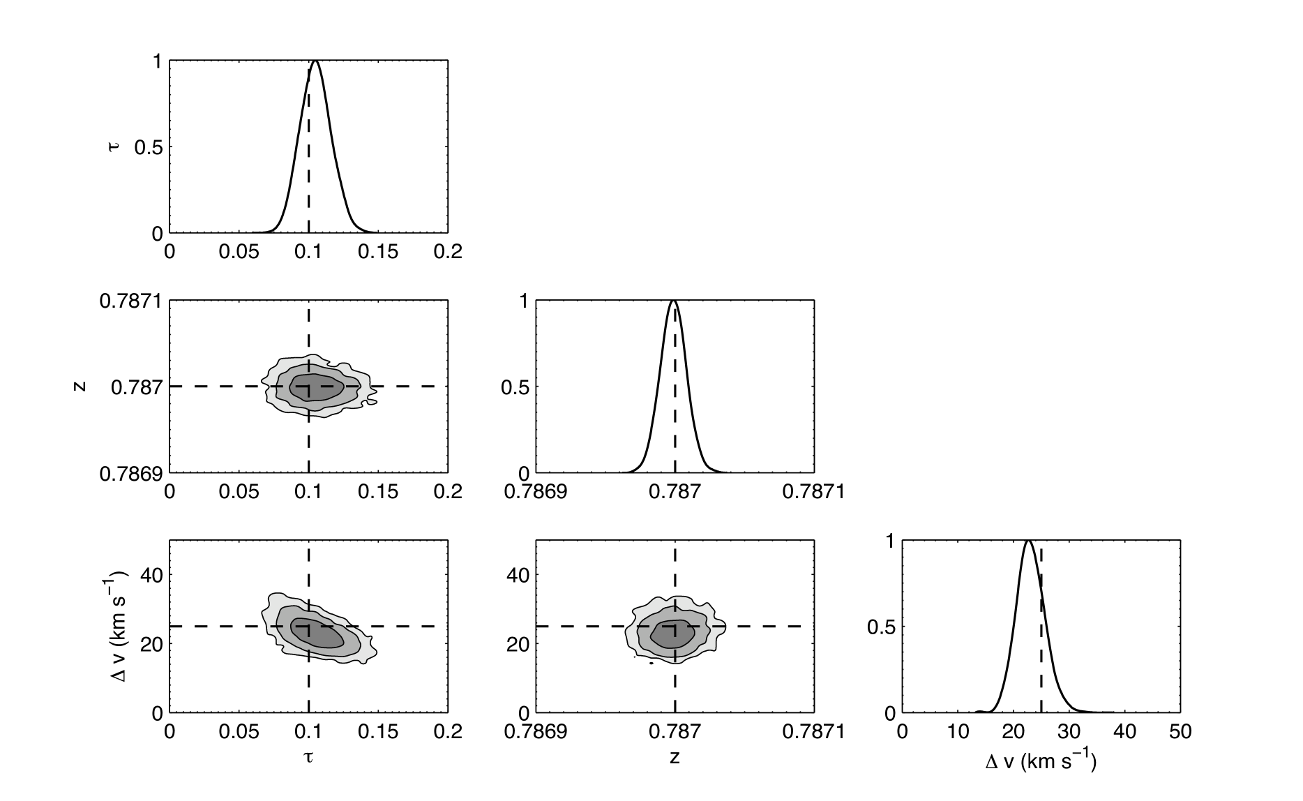
Figure 2 shows an example of the output from line detection in a simulated ASKAP spectrum. In this example one of the two absorption-line components known to be present in the spectrum has been detected above the noise and the posterior probability for the Gaussian parameters estimated. The second absorption-line component at 807.0 MHz ($z=0.760$), while having a relatively wide FWHM of $\Delta v=80$ km s^-1, has a low optical depth of $\tau=0.02$ and so was not detected above the noise. It is clear from the residual spectrum that no other lines are present above the noise level.

For this example spectrum we calculate that $R=60.53\pm 0.07$, indicating that the Gaussian-line model is significantly favoured. The marginalised posterior probability distribution for each parameter is shown in the lower plot in Figure 2 and are reasonably Gaussian in shape. The 2-dimensional contours indicate the correlation between parameters. There is no apparent correlation between the peak optical depth and redshift, or between the FWHM and redshift. There is some anti-correlation between the peak optical depth and FWHM of the line, indicating conservation of the integrated optical depth.

It has been noted that the simulated absorption catalogue was constructed based on a single Gaussian-line model. However when analysing real ASKAP–FLASH data we will have to make an assumption about the analytical form of the line profile. Calculation of the Bayesian evidence statistic provides us with a global likelihood for selecting between competing models. If, for example we choose to parametrise the data using a Lorentizian-line model (including the same uniform priors used for the Gaussian-line model) then we obtain a value of $R=56.88\pm 0.07$. In this case the evidence again rejects the no-line model, but favours the Gaussian-line over the Lorentizan-line model.

Figure 3: The results of running our Bayesian line finder on the simulated ASKAP data cube. Red circles and blue crosses represent detected and undetected lines respectively. Top: Lines of different peak optical depth $\tau$ as a function of the flux density of the background continuum source. The dashed line represents the cut-off for detectability in a 2 hour ASKAP observation as originally estimated by the FLASH team (see text). Bottom: The velocity integrated HI optical depth over the line. The black open stars show published observational data points for radio detections of intervening HI absorption-lines at redshift $z<1$, taken from Table 1 of Curran et al. (2008).

4.2 Comparison with input catalogue

Of the 600 absorption-line components painted onto the 435 brightest sources in the continuum simulation, 60 are found to be at locations off the edge of the main field of the image and are therefore discounted from the sample. Of the components located within the image, there are 3 detections with $R$ less than unity. These detections have comparable significance to the ten false-positive detections and are therefore counted as non-detections. Note that the 10 false-positive detections (which include 4 in absorption and 6 in emission) have very low significance and unphysical velocity widths and hence can be distinguished from the correct detections.

Of the remaining absorption-line components, 76 are detected above the noise with $R$ greater than unity, yielding a detection rate of 14 % from a realistic 2-h integration on an ASKAP field.

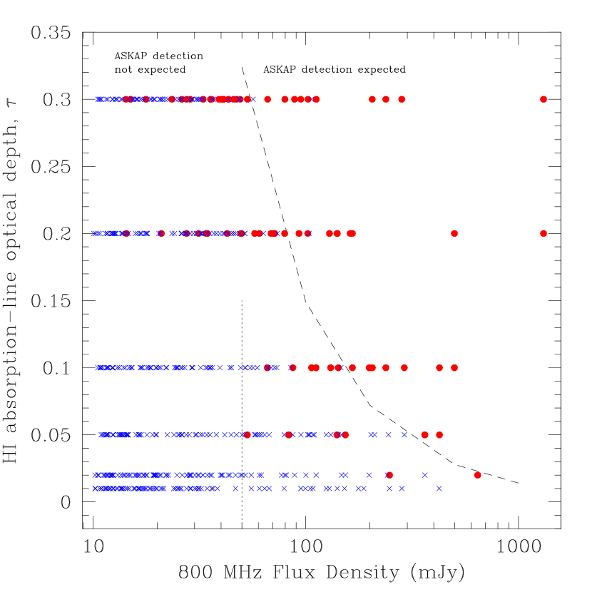
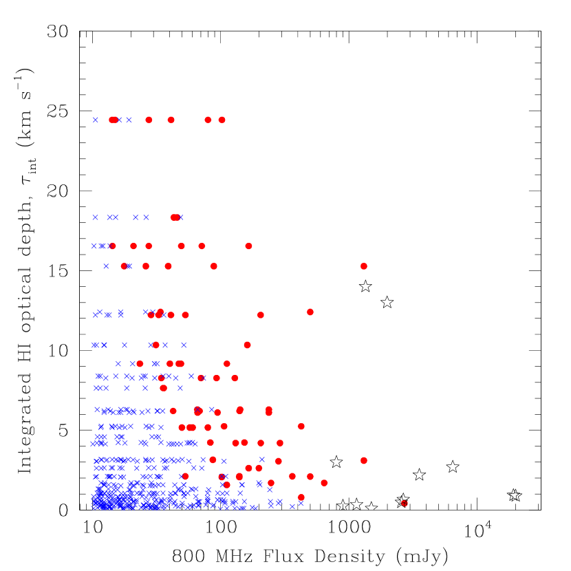
Figure 3 plots the peak and integrated HI optical depth versus the 800 MHz flux density of the background continuum source for both detected and undetected lines from the ASKAP-FLASH simulation The dashed line in the first plot shows the detection limit in peak optical depth $\tau$ originally assumed by the FLASH team, based on the 5-sigma detection of a line peak in a single 18 kHz spectral channel in a 2-h ASKAP observation. We detect almost all of the sources expected to be found in the real ASKAP data, as well as some additional weaker lines. The simulation results therefore imply that the assumed FLASH detection limit is reasonable, and may even be slightly conservative.

The plot of integrated optical depth $\tau_{\mathrm{int}}$ in Figure 3 also shows the existing observational data points for HI absorption-lines at $z<1$ from Table 1 of Curran et al. (2008). This plot shows that the FLASH survey should be able to detect similar HI absorption-lines against continuum sources which are 10-100 times fainter than those typically probed in targeted HI absorption-line searches with existing radio telescopes.

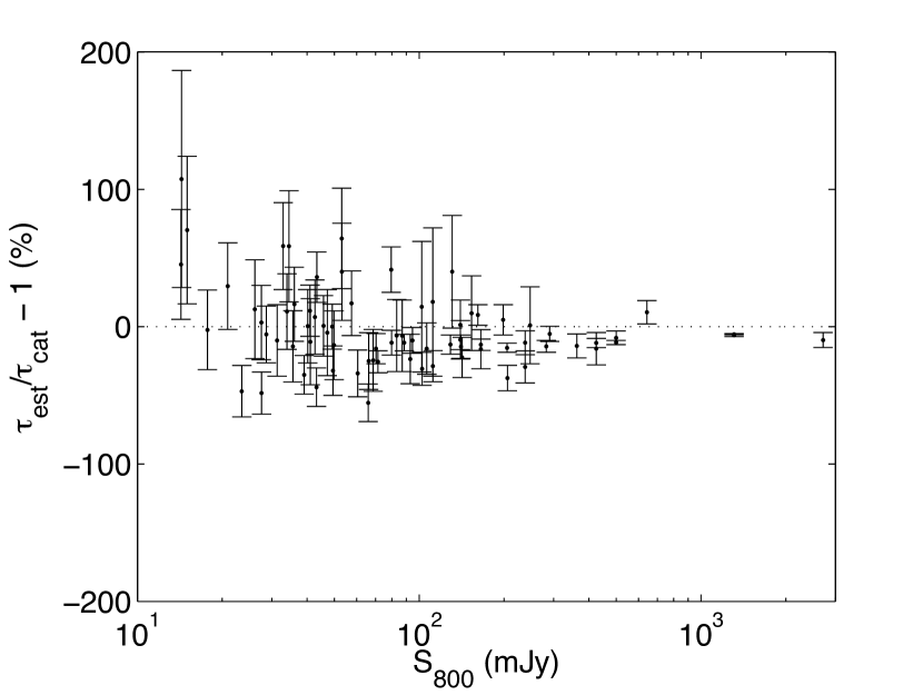
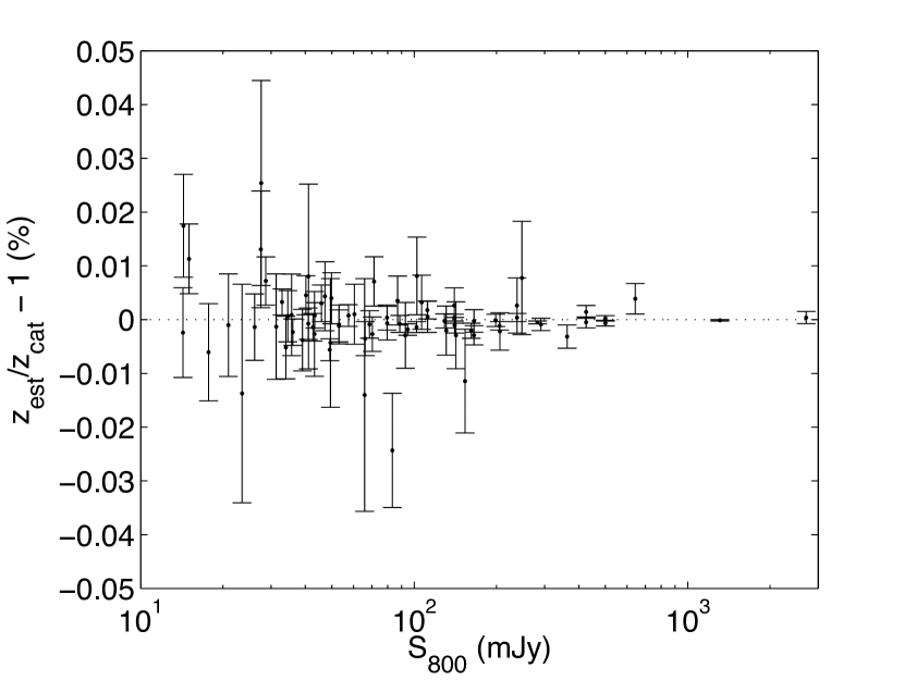
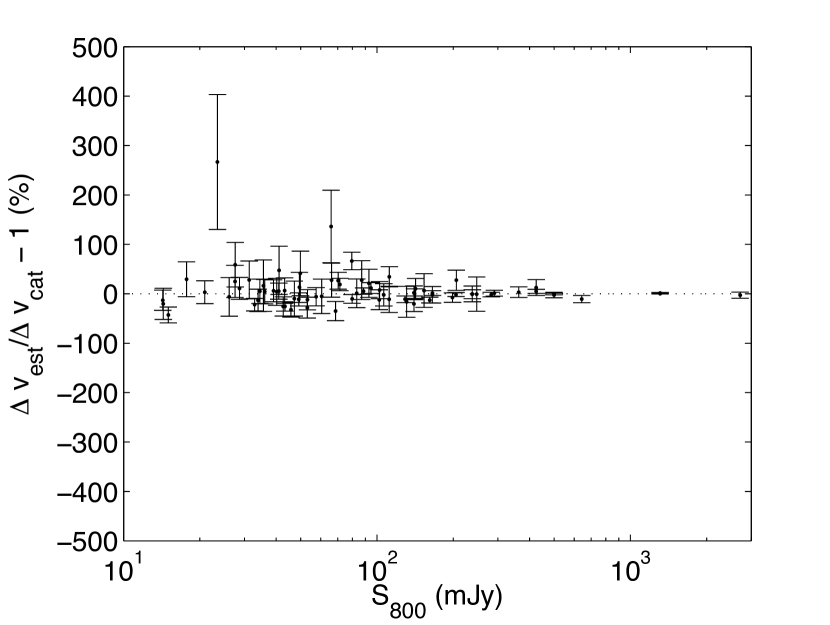
Figure 4 compares the estimated and input catalogue values for each of the absorption-line model parameters, plotted as a function of the continuum source flux density. The redshift position of each line is the most precisely determined parameter from model fitting, with differences compared to the input catologue $\sim 0.01\,\%$. The peak optical depth and FWHM parameters are less precisely determined by model fitting to the simulated data, with differences $\sim 10\,\%$. The large majority of parameters are within $1-3\,\sigma$ of their expected catalogue values. The few significant outliers are likely due to the imaging procedure still in development by the ASKAP computing group. We extract the spectral data from a pixel at the position of the source, and so either pixelisation of the input model or imaging artefacts may produce an offset in the estimated parameters.

Figure 4: Comparison between the estimated and true values for each absorption-line parameter, as a function of the 800 MHz source flux density. Sources located outside of the image edge or with $R$ less than unity are not included in the sample. The errorbars represent the 1 $\sigma$ uncertainty.

4.3 Comparison with DUCHAMP

We searched for absorption-line components in the same set of 435 simulated ASKAP spectra using the Duchamp 3-dimensional source finder (for technical details please refer to Whiting 2008).

This source finder uses an intensity-thresholding algorithm without assuming any underlying analytical model for the source shape or line profile. Duchamp is therefore optimized for detecting complex sources in 3 dimensions rather than simultaneous detection and parametric model fitting of spectral-line profiles.

For this work we are considering the spectral domain and so we ran Duchamp in a mode such that it was optimized for spectral searches (for example we set the parameters searchType and smoothType to “spectral”). The source-finding parameters are optimised so that we minimise the number of false positive detections, while maximising the number of detected absorption-line components. The data are smoothed using a Hanning filter width of 3 and the detections are accepted if they are brighter than a threshold of $3\,\sigma$ above the mean and contain more than 3 contiguous channels. In order to correctly determine the total number of false-positive detections we run the program in both emission and absorption-line mode.

Of the 540 absorption-line components located within the edge of the image, 63 are correctly detected with the Duchamp source finder. We obtain 7 false-positive detections with 3 in absorption and 4 in emission. One of these false positive detections has an unphysical peak optical depth, while the other 6 have relatively low SNR and are indistinguishable from the other correctly detected low-SNR absorption components.

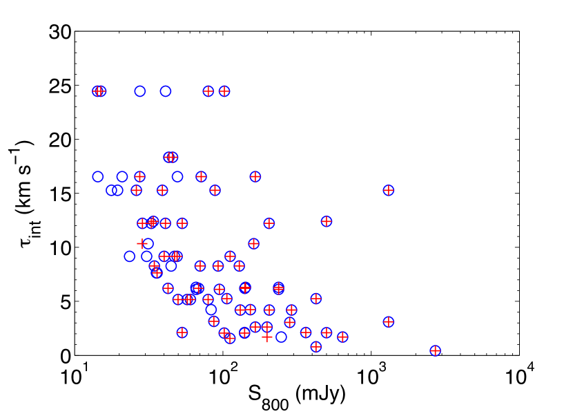
Figure 5 shows the velocity-integrated optical depth versus the 800 MHz source flux density for detected absorption-line components using both the Bayesian line finder and Duchamp. There are 18 absorption-line components that are correctly detected with the Bayesian line finder and not with Duchamp, including 3 which have $R$ less than unity and are hence rejected due to low significance. Both of the absorption-line components that are correctly detected with Duchamp and not with the Bayesian line finder have low SNRs (less than 3) and are therefore difficult to distinguish from the false positives.

Qualitatively, Duchamp requires significantly lower computation time for the 1-dimensional spectral-line finding problem, because calculation of the evidence statistic requires Monte–Carlo integration over a multi-dimensional parameter space (see Equation 3.2). However the Bayesian line finder provides a more robust method for detecting low-significance spectral-lines, estimating the probability distribution of model parameters, and selecting between competing analytical models.

Figure 5: The velocity-integrated optical depth versus 800 MHz source flux density for detected absorption-line components using the Bayesian line finder (Blue Circles) and Duchamp (Red Crosses).

5 Conclusions

We have applied the multi-nested sampling algorithm to simulated ASKAP–FLASH data in order to test its usefulness in both finding and fitting absorption-line components. This Bayesian technique provides us with a robust tool for selecting spectral-line detections in low-SNR data, along the line of sight to known continuum sources. The sampling algorithm is necessarily slower than the Duchamp source finder because it calculates an estimate of the Bayesian evidence statistic, and hence provides us with a method of both assigning significance to our detections and selecting between competing models. Our analysis of a simulated ASKAP data cube also shows that the line-finding techniques presented in this paper can robustly detect HI absorption lines at (and even slightly below) the levels originally estimated by the FLASH team for a two-hour integration with ASKAP.

References

- Allison et al. (2011) Allison J. R., Taylor A. C., Jones M. E., Rawlings S., Kay S. T., 2011, MNRAS, 410, 341
- Condon et al. (1998) Condon J. J., Cotton W. D., Greisen E. W., Yin Q. F., Perley R. A., Taylor G. B., Broderick J. J., 1998, AJ, 115, 1693
- Curran et al. (2008) Curran S. J., Whiting M. T., Wiklind T., Webb J. K., Murphy M. T., Purcell C. R., 2008, MNRAS, 391, 765
- Deboer et al. (2009) Deboer D. R., Gough R. G., Bunton J. D., Cornwell T. J., Beresford R. J., Johnston S., Feain I. J., Schinckel A. E., Jackson C. A., et. al. 2009, IEEE Proceedings, 97, 1507
- Feroz & Hobson (2008) Feroz F., Hobson M. P., 2008, MNRAS, 384, 449
- Feroz et al. (2009) Feroz F., Hobson M. P., Bridges M., 2009, MNRAS, 398, 1601
- Feroz et al. (2009) Feroz F., Hobson M. P., Zwart J. T. L., Saunders R. D. E., Grainge K. J. B., 2009, MNRAS, 398, 2049
- Gupta et al. (2010) Gupta N., Srianand R., Bowen D. V., York D. G., Wadadekar Y., 2010, MNRAS, 408, 849
- Johnston et al. (2007) Johnston S., Bailes M., Bartel N., Baugh C., Bietenholz M., Blake C., Braun R., Brown J., Chatterjee S., Darling J., Deller A., et. al. 2007, PASA, 24, 174
- Kanekar et al. (2009) Kanekar N., Prochaska J. X., Ellison S. L., Chengalur J. N., 2009, MNRAS, 396, 385
- Marshall et al. (2003) Marshall P. J., Hobson M. P., Slosar A., 2003, MNRAS, 346, 489
- Mauch et al. (2003) Mauch T., Murphy T., Buttery H. J., Curran J., Hunstead R. W., Piestrzynski B., Robertson J. G., Sadler E. M., 2003, MNRAS, 342, 1117
- Sivia (2006) Sivia D. S., 2006, Data Analysis: A Bayesian Tutorial., second edn. Oxford University Press, New York
- Skilling (2004) Skilling J., 2004, in Bayesian Inference and Maximum Entropy methods in science and engineering: 24th International Workshop on Bayesian Inference and Maximum Entropy Methods in Science and Engineering Vol. 735, Nested Sampling. pp 395–405
- Wells et al. (1981) Wells D. C., Greisen E. W., Harten R. H., 1981, AAPS, 44, 363
- Whiting (2008) Whiting M. T., 2008, in Koribalski, B. S. & Jerjen, H. ed., Galaxies in the Local Volume Astronomers! Do You Know Where Your Galaxies are?. p. 343
- Wilman et al. (2008) Wilman R. J., Miller L., Jarvis M. J., Mauch T., Levrier F., Abdalla F. B., Rawlings S., Klöckner H., Obreschkow D., Olteanu D., Young S., 2008, MNRAS, 388, 1335