A Characterization of the Combined Effects of Overlap and Imbalance on the SVM Classifier

Abstract

In this paper we demonstrate that two common problems in Machine Learning—imbalanced and overlapping data distributions—do not have independent effects on the performance of SVM classifiers. This result is notable since it shows that a model of either of these factors must account for the presence of the other. Our study of the relationship between these problems has lead to the discovery of a previously unreported form of “covert” overfitting which is resilient to commonly used empirical regularization techniques. We demonstrate the existance of this covert phenomenon through several methods based around the parametric regularization of trained SVMs. Our findings in this area suggest a possible approach to quantifying overlap in real world data sets.

1 Introduction

A data set is imbalanced when its elements are not evenly divided between the classes. In practical applications it is not uncommon to see very high imbalance, where upwards of 90% of the available training data belong to only one class. Overlap is another common problem, which occurs when there are regions of the data space where the posterior class distributions are near equal, even when the priors are known with certainty. In these cases it is difficult to make a principled decision on how to divide the volume of these regions between the classes.

Although the overlap and imbalance problems have been studied previously, (see [6]; [10]; [1]; [3]; [17] for some representative works in this area), work on each problem has happened largely in isolation. Some authors (e.g. [2]; [16]; [14]; and [4]) have performed experiments in the presence of both factors; however, the nature of their interaction is still not well understood. Our finding that their effects are not independent is an important step towards a characterization of how these factors affect classifier performance.

We propose that the behaviour observed in the combined case can be explained by phenomenon we call “covert” overfitting. Covert overfitting is similar in principle to regular overfitting, but the ambiguities which lead to overfitting are present in the generative distributions of the classes, rather than just in the training set. This complication ensures that standard empirical regularization techniques, such as cross validation, or using a separate validation set for testing, are not able to detect this phenomenon. We explore this problem in detail, and offer several demonstrations of its occurrence, in the later sections of this paper.

In the first part of this paper we explore how the Support Vector Machine (SVM) classifier performs when faced with overlapping and imbalanced data sets. In contrast to previous work in this area, we directly address the question of how the relationship between these factors affects classifier performance. A key result of this work is that the effects from these factors are not independent. We show that, although neither factor acting alone has an unexpectedly strong effect, the presence of overlap and imbalance together causes performance degradation which is more severe than we are lead to expect by considering them independently. This is an extension of our previous work on the overlap and imbalance problems in [7], but goes beyond it by offering an explanation and application of the combined effects. We also demonstrate how different signatures of these effects might be used as tools to measure overlap in real world data.

2 Data and Experimental Setup

We build our analysis around a series of synthetic data sets in the from of two dimensional “backbone” models. To generate a data set we sample points form the region $[0,1]\times[0,1]$. The range along one dimension is divided into four regions with alternating class membership, (two regions for each class), while the two classes are indistinguishable in the other dimension (see Figure 1). These domains make a good candidate for study since they are relatively simple, both to visualize and to understand, yet the optimal decision boundary is sufficiently non-linear to cause interesting effects to emerge. The main problems we discuss in this paper often do not appear in very simple domains; we have chosen our models to be sufficiently complex to demonstrate the issues at hand.

Throughout this paper it will be necessary for us to have a parameterization of the overlap and imbalance levels present in a particular data set. This will allow us to study classifier performance with respect to these parameters and to formulate a model of how they affect performance.

Figure 1: Sample backbone models in two dimensions.

We parameterize the overlap level with $\mu\in[0,1]$ such that when $\mu=0$ the two classes are completely separable and when $\mu=1$ both classes are distributed uniformly across the entire domain. Intermediate values of $\mu$ indicate overlap along the region boundaries.

The imbalance level, which we denote $\alpha\in[0.5,1]$, is measured as the proportion of the data set belonging to the majority class. When there is imbalance, we always take the second class as the majority class; however, since the class distributions are symmetric, in these models the distinction between “first” and “second” is somewhat arbitrary, hence our decision to consider only the degree of imbalance and ignore which particular class is present in the majority.

Using this scheme, we generate a series of data sets for each collection of experiments by varying one, or both, of the available parameters. Unless otherwise indicated, all our experiments are repeated using training sets of several different sizes varying (logarithmically) between 25 and 6400 examples (although in the interest of saving space we report only a subset of these results). Testing is done using newly generated data sets of the appropriate imbalance level, overlap level and size.

We assess classifier performance using the F₁-score of the classifier trained on each data set, where the minority class is taken to be positive. The F₁-score is the harmonic mean of the precision and recall of a classifier and is a commonly used scalar measurement of performance. Our choice of positive class reflects the state of affairs present in many real world problems where it is difficult to obtain samples from the class of interest. The F₁-score is one of the family of F_β-scores and treats precision and recall as equally important.

Our experiments here focus on the SVM classifier with an RBF kernel. In all cases parameter selection for the SVM was carried out using the simulated annealing procedure described in [5] to select optimal values for $C$ and $\gamma$.

3 Overlap and Imbalance in Isolation

In this section we look at how overlap and imbalance in isolation affect classifier performance. The purpose of this section is to provide some baseline results which will inform our analysis of the combined effects in Section 4.

3.1 Imbalance

This section shows a series of experiments using varying levels of imbalance. We confirm previous results from [10], which indicate that imbalance in isolation is not sufficient to degrade performance. This suggests that poor performance on imbalanced data sets is caused by other factors such as small disjuncts. (For a discussion of why the imbalance problem is best viewed as an instance of the small disjunct problem see [10], [9], and [11]).

Figure 2: Imbalance in isolation. (a) Shows the SVM performance over a range of imbalance levels. (b) Shows the solution complexity over the same range. (c) Shows how performance varies with training set size at various levels of imbalance. In each case $N$ is the number of training data used. Error bars show one standard deviation about the mean over 10 trials. $N$ is the number data in the training and test sets.

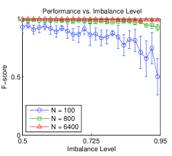
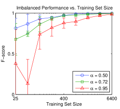
Performance results from our experiments are shown in Figure 2. When the training set size is large we observe that the imbalance level has very little effect on the classifier performance. Performance is only affected when either the imbalance level is very high (and then only slightly), or when there are very few training data. This is exactly what we expect from the existence of small disjuncts in these domains. The influence that the training set size has on performance can be seen explicitly in Figure 2.

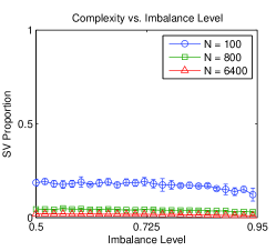
In addition to the F₁-scores, we also recorded the number of support vectors from each run as a measure of the complexity of the trained models. Figure 2 shows the proportion of the training set retained as support vectors and that the imbalance level has no visible adverse effect on the complexity of the SVM solution. In fact, there is a slight drop in complexity when the imbalance level is very high; however, at high levels of imbalance there are very few training data available to support the minority side of the boundary. This interpretation is supported by the fact that as the training set size increases the overall proportion that is retained drops, and the complexity reduction at high imbalance levels becomes less apparent.

The major conclusion that we can draw here is that imbalance in isolation has no adverse affect on the SVM classifier, provided that the training set is sufficiently large. The reduced performance we see when the training set is small can be attributed to the fact that there are not sufficiently many minority examples to infer the class distribution. This is confirmed by the fact that with a large training set the performance is excellent, even on highly imbalanced domains.

3.2 Overlap

In contrast to the imbalance problem, the effects of overlap are not well characterized in the literature (although previous work on the problem can be found in [16]; [14]; and [17]). We use this section to demonstrate that overlapping classes cause the SVM to learn decision boundaries which lack parsimony.

Figure 3 shows performance results with respect to overlap level for a selection of training set sizes, with the explicit relationship between training set size and performance appearing in Figure 3. The experiments which produced these data follow the same procedure as those from Section 3.1, but here we vary the overlap level instead of the imbalance. As in the case of imbalance, we see that very small training sets tend to cause degraded performance; however, in this case the effect is much weaker and becomes less pronounced as the overlap level is increased (see Figure 3). This indicates that, unlike the case of imbalance, when the overlap level is high, it is unlikely that collecting more training data will produce a more accurate classifier.

Figure 3: Overlap in isolation. (a) Shows the SVM performance over a range of overlap levels. (b) Shows the solution complexity over the same range. (c) Shows how performance varies with training set size at various levels of overlap. In each case $N$ is the number of training data used. Error bars show one standard deviation about the mean over 10 trials. $N$ is the number of data in the training and test sets.

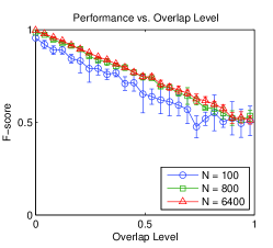
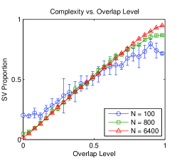
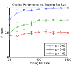
In Figure 3 we see that performance of the SVM classifier in the presence of overlap shows a linear drop as the overlap level is increased, with the linearity becoming more pronounced with larger training sets. An important observation here is that this is precisely what we expect from an optimal classifier on these domains. When we introduce overlap into these (balanced) data sets we create ambiguous regions in the data space where the generative distributions for both classes are near equal. This means that even a classifier with perfect knowledge of the generative distributions will infer near-equal posterior probabilities in these regions, meaning that we cannot predict the class label better than chance.

It is more interesting here to examine the complexity of the SVM solutions, which we again measure using the proportion of the training set retained as support vectors (shown in Figure 3). The response here again appears linear, but in this case a linear response is somewhat alarming. The proportion of the training set retained as support vectors rises linearly as a function of the overlap level, and this effect is visible across a wide range of training set sizes. This indicates that increasing the size of the training set, which was a boon in the case of imbalance, actually causes the SVM solution to increase in complexity.

When overlap is present in isolation, the SVM classifier is able to achieve approximately optimal performance across a wide range of different training set sizes; however, despite the near optimal performance, as the overlap level is increased the complexity of the model rises sharply, both as a function of the overlap level and also as a function of the training set size. This is counter-intuitive, as we generally expect that increasing the amount of training data should lead to “better” models. Due to how we introduce overlap into our distributions the complexity of the optimal solution is independent of the overlap level.

4 Combined Overlap and Imbalance

We now turn our attention to the behavior of the SVM in the presence of both overlap and imbalance simultaneously. We are interested in determining if it is possible to separate the contributions from each factor. If this is possible then we can assign blame for different portions of the performance degradation to each factor; however, if the effects of the two factors interact, this assignment of blame becomes much more complicated and less useful.

If the effects are independent (i.e. they do not interact) then the overlap and imbalance problems can reasonably be studied in isolation; however, if they are not independent it is important to understand the relationship between them, which can only come from studying them together. We will show that this is in fact the case, and our study of the combined effects gives rise to the discovery of a previously unreported phenomenon which we call covert overfitting.

4.1 Test for Independence

We first outline a method to test the hypothesis that overlap and imbalance have independent effects on classifier performance. Let us continue to use $\mu$ as a measure of overlap and $\alpha$ as a measure of imbalance. The hypothesis can be expressed mathematically as the assumption that the performance surface with respect to $\mu$ and $\alpha$ obeys the relation

$$\mathrm{d}P(\mu,\alpha)=f^{\prime}(\mu)\,\mathrm{d}\mu+g^{\prime}(\alpha)\,\mathrm{d}\alpha\enspace,$$

where $f^{\prime}$ and $g^{\prime}$ are unknown functions. That is, we expect the total derivative of performance to be separable into the components contributed by each of $\mu$ and $\alpha$. This hypothesis of independence leads us to expect that we can consider the partial derivatives as functions of a single variable, i.e.

$$\frac{\partial}{\partial\mu}P =f^{\prime}(\mu)\enspace,$$

$$\frac{\partial}{\partial\alpha}P =g^{\prime}(\alpha)\enspace.$$

The functions $f^{\prime}$ and $g^{\prime}$ may not have simple or obvious functional forms, meaning that we cannot compute their values analytically; however, if $f^{\prime}$ and $g^{\prime}$ are known we can find a predicted value for $P(\alpha,\mu)$, up to an additive constant, by evaluating

$$P(\mu,\alpha)=\int f^{\prime}(\mu)\,\mathrm{d}\mu+\int g^{\prime}(\alpha)\,\mathrm{d}\alpha+C\enspace.$$ (1)

Specific values for $P(\mu,\alpha)$ can be computed numerically by training a classifier on a data set with the appropriate level of overlap and imbalance. Since we expect the partial derivatives of $P(\mu,\alpha)$ to be independent, we can compute values for $f^{\prime}$ by evaluating $P(\mu,\alpha)$ for several values of $\mu$ while holding $\alpha$ constant and taking a numerical derivative. Values for $g^{\prime}$ can be computed in a similar manner by holding $\mu$ constant and varying $\alpha$. These values can then be combined into predicted values for $P(\mu,\alpha)$ using (1). Comparing the predicted values for $P(\mu,\alpha)$ to the observed values will allow us to determine if our hypothesis of independence is sound.

Figure 4: Diagram of the proposed independence test.

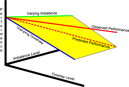
The procedure for applying this model is illustrated in Figure 4, which shows a performance surface parameterized by the overlap and imbalance levels of the training set. First, we take measurements of this surface along the indicated axis-aligned sections. This corresponds to measuring the effects of each factor in isolation, the results of which where shown in previous sections. These data, combined with the model of independence we have described here, allow us to make predictions for the combined case (the dashed line in Figure 4). Comparing these predicted values to the performance of actual classifiers trained on data sets with the corresponding levels of overlap and imbalance enables us to assess the correctness of the model. What we are looking for is a discrepancy between the model’s predictions and our observations (shown in the figure as the difference between the solid and dashed lines). If the predictions do not match well with our observations we can reject the model and conclude that there must be an interaction between the effects of overlap and imbalance on SVM performance.

4.2 Results

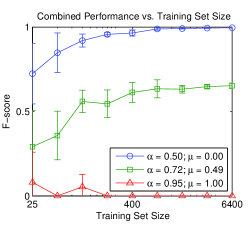
Comparisons between our model predictions and the observed performance on domains with combined overlap and imbalance are shown in Figure 5. These results clearly show that when the training set size is large, the performance predicted by assuming that overlap and imbalance are independent is very different than what is observed. On the other hand, when the training set is small the predictions are quite accurate, showing only a small (but still significant) deviation from the observed results.

Figure 5: Comparing model predictions to observations in the combined case. In these figures the lower x-axis shows the degree of overlap and the upper x-axis shows the degree of imbalance. $N$ is the number of data in the training and test sets.

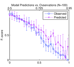
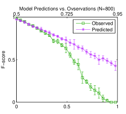
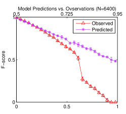
In addition to showing performance which falls short of our model’s predictions, we see a sudden breaking point in performance beyond a certain level of combined overlap and imbalance. This effect is most pronounced when the training set is large, becoming less noticeable with fewer training data and disappearing entirely when the training set size is very small. This drop occurs consistently at approximately $\mu=0.6$ and $\alpha=0.78$ with very little variation across different training set sizes. In [7] we showed that the differences are statistically significant and that the drop is correlated with the peak complexity of these models.

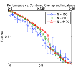
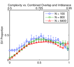
Figure 6 shows the performance and complexity we observed in the combined case across several training set sizes. The data are presented here in the same format as Figures 2 and 3 for ease of comparison. These figures emphasize the breaking point in performance we see with combined overlap and imbalance. Crucially, we see that the performance beyond this breaking point is unchanged across the range of training set sizes we tested; however, more data can significantly improve the pre-breaking-point performance.

Figure 6: Combined overlap and imbalance. In these figures the lower x-axis shows the degree of overlap and the upper x-axis shows the degree of imbalance. $N$ is the number of data in the training and test sets.

The model from Section 4.1 relies only on the independence of the imbalance and overlap problems in order to make predictions for performance in the combined case. Since we have shown that the model predictions are very poor, it is reasonable to conclude that the underlying assumption is incorrect; specifically, we claim that our results demonstrate that there is an interdependence between the effects of overlap and imbalance. The later sections of paper are devoted to characterizing this interdependence.

5 Covert Overfitting

In this section we propose an explanation for the performance and complexity behaviours we observe in the presence of overlap and imbalance. So far we have seen that:

• Imbalance, in isolation, is not a significant problem for SVMs. When there are sufficiently many training data available the SVM forms simple models (as expected, given the simplicity of our domains) which show excellent performance, even when the degree of imbalance is very high.

• Overlap, in isolation, causes SVMs to build very complex models which exhibit performance comparable to an optimal classifier. Although performance drops as the overlap level is increased, it is still optimal since the presence of overlap creates ambiguous regions where even an optimal classifier cannot predict the class label better than chance. However, the complexity of these models is extremely high, especially considering that the complexity required to achieve this performance is no different from the separable case.

• When both factors are present in tandem not only does the SVM build overly complex models, as in the case of overlap in-isolation, but the performance on these domains is also significantly reduced.

Since the underlying reasons for the behaviour in the case of imbalance in isolation is fairly well understood (see the beginning of Section 3.1 for references) we will focus on the remaining two cases here.

We hypothesize that the observed behaviour is a result of a phenomenon we call covert overfitting. Covert overfitting is similar to ordinary overfitting, in that it is a result of mistaking aberrations in the training data for characteristics of the generative class distributions. The key difference is that covert overfitting occurs in the ambiguous regions caused by overlap.

Figure 7: A cartoon example of covert overfitting, where the dotted lines delimit an ambiguous region of the feature space. On the left we see the “optimal” solution and on the right we see a solution where the classifier has overfit. Unlike the case of ordinary overfitting we expect both class boundaries to behave similarly in generalization, since in the ambiguous region only the volume of the feature space assigned to each class will affect performance.

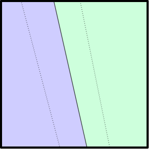
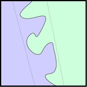
Since it is difficult to make a principled choice of where to place the boundary in an ambiguous region, the task of identifying covert overfitting is more difficult than its ordinary counterpart. Techniques like cross validation, which estimate the generalization performance by testing the classifier on data which was not used during training, are able to detect overfitting in unambiguous regions since an overfit model will not generalize to good performance on the test data. Contrastingly, in ambiguous regions, many different boundaries will achieve comparable generalization performance, since the posterior class probabilities in these regions are nearly equal. This means that we cannot distinguish between parsimonious and overfit solutions in ambiguous regions based on generalization performance alone.

We demonstrate that covert overfitting occurs using two different methods. Both of these methods rely on our ability to apply different degrees of smoothing to the boundary produced by a trained SVM. We present a regularization technique here adapted from [12] (with previous work appearing in [8] and [13]). The key insight allowing this method to function is a result of Liang’s work; however, we have enhanced the algorithm to allow SVM approximations using an arbitrary number of support vectors to be constructed in a single step. While the algorithm in [12] removes one support vector per iteration, we are able to identify a subset of arbitrary size to remove while still maintaining the important properties of the algorithm.

5.1 Spectral Reduction

Given an SVM, we can express the hyperplane normal vector $\boldsymbol{\mathrm{w}}$, as a function of the support vectors [15, chap. 7.3]. Let the support vectors be indexed by a set $N$ and suppose we can partition $N$ into two disjoint subsets, $I$ and $D$, such that $\mathcal{I}=\{\boldsymbol{\mathrm{x}}_{i}:i\in I\}$ is a linearly independent set and the elements of $\mathcal{D}=\{\boldsymbol{\mathrm{x}}_{j}:j\in D\}$ are linearly dependent on the elements of $\mathcal{I}$. Also, define the function $\operatorname{Proj}_{\mathcal{I}}(\boldsymbol{\mathrm{x}})$ as the projection of $\boldsymbol{\mathrm{x}}$ into the span of $\mathcal{I}$. Following Liang, we can write:

$$\boldsymbol{\mathrm{w}} =\sum_{i\in N}\alpha_{i}y_{i}\boldsymbol{\mathrm{x}}_{i}$$

$$=\sum_{i\in I}\alpha_{i}y_{i}\boldsymbol{\mathrm{x}}_{i}+\sum_{j\in D}\alpha_{j}y_{j}\boldsymbol{\mathrm{x}}_{j}$$

$$=\sum_{i\in I}\alpha_{i}y_{i}\boldsymbol{\mathrm{x}}_{i}+\sum_{j\in D}\alpha_{j}y_{j}\operatorname{Proj}_{\mathcal{I}}(\boldsymbol{\mathrm{x}}_{j})$$

$$=\sum_{i\in I}\alpha_{i}y_{i}\boldsymbol{\mathrm{x}}_{i}+\sum_{j\in D}\alpha_{j}y_{j}\bigg{(}\sum_{i\in I}\beta_{ji}\boldsymbol{\mathrm{x}}_{i}\bigg{)}$$

$$=\sum_{i\in I}\alpha_{i}y_{i}\boldsymbol{\mathrm{x}}_{i}+\sum_{i\in I}\sum_{j\in D}\alpha_{j}y_{j}\beta_{ji}\boldsymbol{\mathrm{x}}_{i}$$

$$=\sum_{i\in I}\bigg{(}\alpha_{i}y_{i}+\sum_{j\in D}\alpha_{j}y_{j}\beta_{ji}\bigg{)}\boldsymbol{\mathrm{x}}_{i}$$

$$\triangleq\sum_{i\in I}(\alpha_{i}y_{i})^{\prime}\boldsymbol{\mathrm{x}}_{i}\enspace,$$

where the last equality defines $(\alpha_{i}y_{i})^{\prime}$. Here $\beta_{ji}$ represents the $i$th coordinate of $\boldsymbol{\mathrm{x}}_{j}$ with respect to $\mathcal{I}$. This derivation shows that any linearly dependent support vectors can be eliminated from the SVM by making an appropriate change to the Lagrange multipliers for the remaining independent support vectors. If we restrict $|\mathcal{I}|$ in the above derivation to be less than the dimensionality of the span of the support vectors then the third equality becomes an approximation (since $\mathcal{D}$ will no longer be linearly dependent on $\mathcal{I}$) and we find, following Liang, that provided we select $\mathcal{I}$ so as to minimize $\sum_{j\in D}||\operatorname{Proj}_{\mathcal{I}}(\boldsymbol{\mathrm{x}}_{j})-\boldsymbol{\mathrm{x}}_{j}||$, the resulting SVM is the best approximation of the original, using $|\mathcal{I}|$ support vectors.

It is important to note at this point that the $\boldsymbol{\mathrm{x}}_{i}$ in the above derivation must be expressed in the implicit space induced by the kernel. This complicates matters since this space may be very high, or even infinite, dimensional. Thus, we need a method which does not require us to compute explicit representations for the support vectors in the implicit space.

The solution to this problem is offered by the kernel matrix. The kernel matrix for an SVM with $n$ support vectors is an $n\times n$ symmetric matrix $\boldsymbol{\mathrm{Q}}$, such that

$$\boldsymbol{\mathrm{Q}}_{ij}=K(\boldsymbol{\mathrm{x}}_{i},\boldsymbol{\mathrm{x}}_{j})\enspace,$$

where the $\boldsymbol{\mathrm{x}}_{i}$ are the support vectors and $K(\cdot,\cdot)$ is the kernel function. The kernel matrix is the Gram matrix of the support vectors, after applying the implicit mapping implied by the kernel function, and encodes important information about the SVM. For instance, since the kernel matrix is a Gram matrix, $\operatorname{rank}(\boldsymbol{\mathrm{Q}})$ is equal to the number of linearly independent support vectors. Furthermore, if we find a linearly independent spanning subset of the rows of $\boldsymbol{\mathrm{Q}}$, we can take the corresponding support vectors as a minimal set of support vectors required to re-express $\boldsymbol{\mathrm{w}}$ as in the above derivation. In this way the original problem is reduced to finding a subset of the rows of $\boldsymbol{\mathrm{Q}}$ which form a basis for its row space.

This basis can be found efficiently by computing the $\boldsymbol{\mathrm{LUP}}$ decomposition of $\boldsymbol{\mathrm{Q}}$. This gives a lower triangular matrix $\boldsymbol{\mathrm{L}}$, an upper triangular matrix $\boldsymbol{\mathrm{U}}$, and a permutation matrix $\boldsymbol{\mathrm{P}}$, such that $\boldsymbol{\mathrm{P}}\boldsymbol{\mathrm{Q}}=\boldsymbol{\mathrm{L}}\boldsymbol{\mathrm{U}}$. The matrices $\boldsymbol{\mathrm{L}}$ and $\boldsymbol{\mathrm{U}}$ are not useful to us; however, the matrix $\boldsymbol{\mathrm{P}}\boldsymbol{\mathrm{Q}}$ has the useful property that its first $\operatorname{rank}(\boldsymbol{\mathrm{Q}})$ rows are linearly independent. Since $\boldsymbol{\mathrm{P}}$ is a permutation matrix, we see immediately that we can use it to identify the rows of $\boldsymbol{\mathrm{Q}}$ we require.

The preceding paragraph shows that we can use a linearly independent subset of the rows of $\boldsymbol{\mathrm{Q}}$ to select a minimal set of support vectors which can be used to produce an exact reconstruction of the original SVM. We now address the problem of identifying which support vectors we can remove to produce an optimal rank-reduced approximation of the original. The goal is to be able to select an arbitrary number of support vectors and to have a method which we can use to construct the best possible approximation to our original SVM using the specified number of support vectors, selected from among the support vectors of the original.

The key here is to notice that, since $\boldsymbol{\mathrm{Q}}$ is a symmetric matrix, we can take its eigenvalue decomposition

$$\boldsymbol{\mathrm{Q}}=\boldsymbol{\mathrm{V}}\boldsymbol{\mathrm{\Lambda}}\boldsymbol{\mathrm{V}}^{\mathrm{T}}\enspace,$$

where $\boldsymbol{\mathrm{V}}=[\boldsymbol{\mathrm{v}}_{1}\cdots\boldsymbol{\mathrm{v}}_{n}]$ is an orthogonal matrix of eigenvectors and $\boldsymbol{\mathrm{\Lambda}}=\operatorname{diag}(\lambda_{1},\cdots,\lambda_{n})$ is a diagonal matrix of eigenvalues. For convenience we can require the eigenvalues are ordered such that $\lambda_{i}\geq\lambda_{i+1}$. If we let $r=\operatorname{rank}(\boldsymbol{\mathrm{Q}})$ then we can rewrite this decomposition as

$$\boldsymbol{\mathrm{Q}}=\sum_{i=1}^{n}\lambda_{i}\boldsymbol{\mathrm{v}}_{i}\boldsymbol{\mathrm{v}}_{i}^{\mathrm{T}}=\sum_{i=1}^{r}\lambda_{i}\boldsymbol{\mathrm{v}}_{i}\boldsymbol{\mathrm{v}}_{i}^{\mathrm{T}}\enspace,$$ (2)

where the second equality holds since $\lambda_{r+1}=\dotsi=\lambda_{n}=0$. We can use (2) to form approximations of $\boldsymbol{\mathrm{Q}}$ by truncating the sum after some $r^{\prime}<r$ terms, giving

$$\boldsymbol{\mathrm{Q}}^{\prime}=\sum_{i=1}^{r^{\prime}}\lambda_{i}\boldsymbol{\mathrm{v}}_{i}\boldsymbol{\mathrm{v}}_{i}^{\mathrm{T}}\enspace,$$

which is the best rank-$r^{\prime}$ approximation of $\boldsymbol{\mathrm{Q}}$.

Since $\boldsymbol{\mathrm{Q}}^{\prime}$ is an $n\times n$ matrix with rank $r^{\prime}<n$ we can select $r^{\prime}$ linearly independent rows of $\boldsymbol{\mathrm{Q}}^{\prime}$ which give a basis for its row space. Since $\boldsymbol{\mathrm{Q}}^{\prime}$ is the best rank-$r^{\prime}$ approximation of $\boldsymbol{\mathrm{Q}}$, it follows that the $r-r^{\prime}$ dimensions of $\boldsymbol{\mathrm{Q}}$’s row space not represented in $\boldsymbol{\mathrm{Q}}^{\prime}$ are the dimensions which provide the least contribution to $\boldsymbol{\mathrm{Q}}$. Since there is a 1-1 correspondence between the dimensionality of the kernel row space and the number of support vectors required to represent the SVM hyperplane, selecting linearly independent rows of $\boldsymbol{\mathrm{Q}}^{\prime}$ corresponds to selecting support vectors whose presence has a large effect on the hyperplane.

We now have sufficient information to construct rank-reduced approximations of a given SVM. Training an SVM in the usual way gives us a set of support vectors and their corresponding Lagrange multipliers. To construct an approximation of this SVM using $r^{\prime}$ support vectors we construct the kernel matrix, $\boldsymbol{\mathrm{Q}}$ and its best rank-$r^{\prime}$ approximation, $\boldsymbol{\mathrm{Q}}^{\prime}$. Identifying a subset of the rows of $\boldsymbol{\mathrm{Q}}^{\prime}$ which form a basis for its row space tells us which of the support vectors to keep in the reduced model (there will be exactly $r^{\prime}=\operatorname{rank}(\boldsymbol{\mathrm{Q}}^{\prime})$ of them). We then update the Lagrange multipliers using the rule,

$$(\alpha_{i}y_{i})^{\prime}\coloneqq\alpha_{i}y_{i}+\sum_{j\in D}\alpha_{j}y_{j}\beta_{ji}\enspace.$$ (3)

The new SVM, with support vectors selected using the $\boldsymbol{\mathrm{LUP}}$ decomposition of $\boldsymbol{\mathrm{Q}}^{\prime}$ and Lagrange multipliers given by (3), is the best approximation of the original SVM using $r^{\prime}$ support vectors.

The procedure described in this section can be used to produce arbitrary rank-reduced approximations of a trained SVM. This gives us access to an entire spectrum of increasingly more regularized versions of the SVM model. In the following sections we exploit this ability to gradually regularize our model in order to demonstrate the existence of covert overfitting.

5.2 Hyperplane Angles

The SVM is, at its core, a linear classifier. The ability to handle non-linear problems comes from the kernel, which performs an implicit mapping into a high dimensional feature space. In this implicit space, the SVM decision boundary is represented as the zero level-set of a linear function. Since the function is linear, it can be described by its normal vector and so the similarity of two SVM models can be measured by the angle between the normal vectors of their corresponding hyperplanes.

We must avoid computing the normal vectors directly, since the dimensionality of the implicit space may be very high or even infinite. Nonetheless, it is still possible to compute the angle between two SVM hyperplanes in the implicit space without computing their representations explicitly.

In general, ignoring the constant term for simplicity, an SVM hyperplane is given by

$$f(\boldsymbol{\mathrm{x}})=\sum_{i=1}^{r}\alpha_{i}y_{i}\langle\boldsymbol{\mathrm{x}}_{i},\boldsymbol{\mathrm{x}}\rangle=\boldsymbol{\mathrm{\alpha}}\boldsymbol{\mathrm{X}}\boldsymbol{\mathrm{x}}^{\mathrm{T}}=\boldsymbol{\mathrm{w}}\boldsymbol{\mathrm{x}}^{\mathrm{T}}\enspace,$$

where $\boldsymbol{\mathrm{\alpha}}_{i}=\alpha_{i}y_{i}$, $\boldsymbol{\mathrm{X}}$ is a matrix with the support vectors (represented in the implicit space) as its rows, and $\boldsymbol{\mathrm{w}}$ is the hyperplane normal vector. Crucially, the final equality shows that $\boldsymbol{\mathrm{w}}=\boldsymbol{\mathrm{\alpha}}\boldsymbol{\mathrm{X}}$, which we do not want to compute directly (since $\boldsymbol{\mathrm{X}}$ is a matrix of vectors in the implicit space), but we can use to compute the inner product of hyperplane normals.

Suppose now that we have two SVMs, with hyperplane normals given by $\boldsymbol{\mathrm{w}}_{1}=\boldsymbol{\mathrm{\alpha}}_{1}\boldsymbol{\mathrm{X}}_{1}$ and $\boldsymbol{\mathrm{w}}_{2}=\boldsymbol{\mathrm{\alpha}}_{2}\boldsymbol{\mathrm{X}}_{2}$ the angle between them is

$$\cos(\theta) =\frac{\boldsymbol{\mathrm{w}}_{1}\boldsymbol{\mathrm{w}}_{2}^{\mathrm{T}}}{\boldsymbol{\mathrm{w}}_{1}\boldsymbol{\mathrm{w}}_{1}^{\mathrm{T}}\boldsymbol{\mathrm{w}}_{2}\boldsymbol{\mathrm{w}}_{2}^{\mathrm{T}}}=\frac{\boldsymbol{\mathrm{\alpha}}_{1}\boldsymbol{\mathrm{X}}_{1}\boldsymbol{\mathrm{X}}_{2}^{\mathrm{T}}\boldsymbol{\mathrm{\alpha}}_{2}^{\mathrm{T}}}{\boldsymbol{\mathrm{\alpha}}_{1}\boldsymbol{\mathrm{X}}_{1}\boldsymbol{\mathrm{X}}_{1}^{\mathrm{T}}\boldsymbol{\mathrm{\alpha}}_{1}^{\mathrm{T}}\boldsymbol{\mathrm{\alpha}}_{2}\boldsymbol{\mathrm{X}}_{2}\boldsymbol{\mathrm{X}}_{2}^{\mathrm{T}}\boldsymbol{\mathrm{\alpha}}_{2}^{\mathrm{T}}}\enspace.$$

This expression is in terms of the inner products of the rows of $\boldsymbol{\mathrm{X}}_{1}$ and $\boldsymbol{\mathrm{X}}_{2}$ (i.e. inner products of support vectors in the implicit space) which can be computed efficiently using the kernel function. The $\boldsymbol{\mathrm{X}}_{1}\boldsymbol{\mathrm{X}}_{2}^{\mathrm{T}}$ term requires that both SVMs use the same kernel in order for this method to work. Since different kernels imply implicit mappings into different spaces, so the notion of an “angle” between the hyperplanes loses meaning when different kernels are used.

The method described here can be used to measure the angle between an SVM and a rank-reduced approximation of the same model. We expect that higher rank approximations will produce hyperplanes which converge to the original (this follows directly from our regularization method); however, what we are interested in is the rate of convergence and more importantly, how the angle compares to performance. If covert overfitting is present we expect the performance of the rank-reduced models to converge to the performance of the original much faster than the angle between their hyperplanes converges to 0.

5.3 Class Assignment Variation

If an SVM has placed its boundary in an ambiguous region, it should be possible to move the boundary within this region without affecting the performance of the classifier. This suggests a method for identifying covert overfitting by watching for a plateau in performance as the kernel rank is reduced. Since our smoothing method guarantees that we move the boundary as little as possible at each iteration, we expect that the first support vectors to be removed are those which encode information in the most complex regions of the boundary (which we expect to correspond to those regions where covert overfitting has occurred). If these details represent true features of the problem (i.e. the true class boundary is in fact complex in this region) then smoothing the SVM solution will cause a drop in performance; however, if details removed by the smoothing process are a result of covert overfitting then we expect the performance to remain approximately constant as they are removed.

If there are data points near the boundary, it is quite likely that small changes in the boundary position will cause their predicted label to change. This will happen regardless of whether or not the boundary correctly encodes the optimal separating line between the classes. Thus, we can look for the combined occurrence of two effects as an indication of covert overfitting:

1. The SVM rank must be substantially reduced before we see a significant drop in performance, and

2. There are many test data which have their predicted label change frequently as the rank drops.

Neither of these effects in isolation are sufficient to detect covert overfitting. If the classes are highly separated then it may be possible to reduce the rank substantially without affecting performance, as the boundary is free to move within the large margin; however, in this case we would not see variation in label assignment. Conversely, if we see varying label assignments but performance drops, then we are likely losing important information about the true class boundary, rather than details from covert overfitting. If the effects are present together then the constant performance indicates that the overall predictive power of the model is maintained, while at the same time the label assignment changes indicate that the boundary is moving in a region with a small margin.

5.4 Results

In order to demonstrate the existance of covert overfitting we built a synthetic data set with an overlap level of 0.4 and an imbalance level of 0.6, following the same procedure as for the previous experiments. We then trained an SVM classifier on this data set, using the simulated annealing procedure from [5], with cross validation to select parameter values. After an initial pre-processing step to remove redundant support vectors, we construct a series of rank-reduced approximations using the method described in Section 5.1. We use each of these rank-reduced SVMs to classify a test set drawn from the same generative distribution that was used for training. For each rank-reduced SVM we measure the angle between its hyperplane and that of the original SVM, and record which elements of the test set have their class assignment change as each support vector is removed.

To decide when the original SVM is sufficiently well approximated by a rank-reduced approximation, we compare the rank-reduced performance to the original performance. We consider the rank-reduced SVMs to be accurate reconstructions of the original if their test performance is greater than or equal to $p-\delta$, where $p$ is the performance of the original classifier and $\delta$ is some small threshold. We call the lowest-rank for which this occurs the sufficiency point and for our tests we chose $\delta=0.001$. We are most interested in the behaviour of the reconstructions with rank greater than the sufficiency point, as these are the ones which we expect to show variation within the ambiguous region.

Figure 8: Covert Overfitting Results. (a) Compares performance (solid line) to the angle between the original SVM and it’s rank reduced approximations (dashed line). (b) Compares performance to label assignment changes over the same domain (see the text for a complete description of this figure). The vertical line in both figures indicates the sufficiency point.

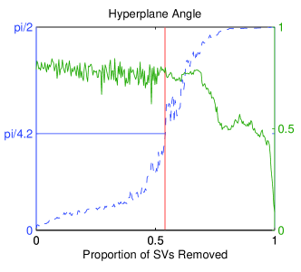
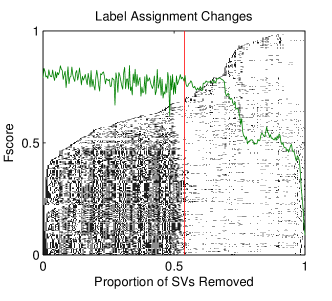
Figure 8 shows an overlaid plot of the performance of the rank-reduced reconstructions and the angle between the original and approximated hyperplanes. The vertical line in the figures shows the sufficiency point. What should be immediately striking here is that not only can more than half the support vectors be removed without significantly altering the performance, but the angle between the original hyperplane and the rank-reduced hyperplane at the sufficiency point is quite large.

As the kernel rank increases, the convergence (in angle) of the reconstructed hyperplanes towards the original is mostly smooth and monotonic, which is exactly what we expect from the reduction method. However, since the performance beyond the sufficiency point is fairly constant, and the angle between the reconstructed hyperplane and the original at the sufficiency point is large, it follows that there is a significant amount of information represented by the original SVM which is not necessary to achieve comparable performance.

This effect—the representation of additional information beyond what is required to achieve good performance—is an example of what we expect from ordinary overfitting. The difference here is that the test performance is not reduced by this behaviour, as the “extra” information in the training set which caused the overfitting is present in the test set as well. Because the training and test sets exhibit the same systematic problem, we cannot detect this phenomenon through validation of the performance alone.

Figure 8 shows the performance of the rank-reduced SVM approximations overlaid on a visualization of the class assignment variation as the rank of the reconstruction is changed. To create this visualization, we divide the area of the figure into a grid of cells, where the rows correspond to elements of the test set and the columns correspond to the different kernel ranks. Each cell is shaded black if reducing the SVM rank by one causes the label assigned to the corresponding element of the training set to change. Note that this does not indicate if the label is correctly assigned, but instead tracks when removing a support vector causes the SVM to “change its mind” about which label should be assigned to each test instance. For ease of interpretation the data have been sorted along the vertical axis, ordered by the largest rank which causes their label to change. Again, we are interested in the behaviour of class assignments when the rank is greater than the sufficiency point.

In this case we can again see the effects of covert overfitting. In fact, we see that the majority of the variation in label assignment takes place after the sufficiency point, where performance is relatively constant. We repeated this experiment on a variety of different backbone models, with varying levels of overlap and imbalance, and we found that this behaviour is consistent. The number of test data whose label is changed before the sufficiency point is high when there is strong overlap, and the frequency of label assignment changes is typically densest in this region as well.

What remains unclear at this point is to what degree the variation is localized to the ambiguous regions. We have demonstrated that there is movement in the SVM hyperplane beyond the sufficiency point, and that this hyperplane movement causes significant changes in how the SVM assigns labels to test data, despite the performance remaining constant. However, it is possible that the label changes we are seeing are spread uniformly across the entire domain.

To show that the label changes are in fact localized in the ambiguous regions, we select the test data whose label is changed at least once after the sufficiency point has been reached and check if they are localized to the ambiguous region. Figure 9 shows the distribution of these data along the dimension in which they are distinguishable (recall from Section 2 that our 2D backbone models are indistinguishable in only one dimension). The distribution is clearly localized in the ambiguous regions with some additional variation near the boundaries (e.g. note the behaviour around the crisp boundary at 0.5).

Figure 9: A demonstration that covert overfitting is localized to the ambiguous regions of the data space. (a) Shows the distribution of test data with at least one label change with rank higher than the sufficiency point. The boxes in the diagram delimit ambiguous regions. (b) Shows the proportion of label changes localized to the ambiguous regions at various degrees of smoothing.

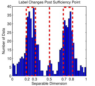
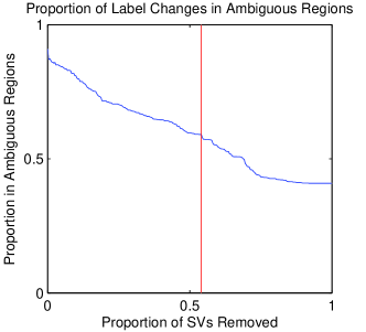
Figure 9 demonstrates that the degree of localization of label variations to the ambiguous regions across several degrees of smoothing. The trend line in this figure shows, for each level of smoothing, the proportion of test data which have had their label assignment change at least once and lie in an ambiguous region. When the rank is extremely low the proportion is approximately 0.42, which is equal to the proportion of the entire test set which lies in an ambiguous region; however, we see that when we consider high rank approximations the label changes are highly localized to the ambiguous regions.

6 Conclusion

In this paper we first looked at how the overlap and imbalance problems in isolation affect performance of the SVM classifier. In the case of imbalance we saw that when there are sufficiently many training data, imbalance does not degrade the SVM performance. We also saw, in the case of overlap in isolation, that even when there are ambiguous regions in the data space, the SVM is still able to achieve approximately optimal performance. Naturally, in this case the overall performance is significantly lower than the imbalanced case, but this is a result of inherent ambiguity in the data themselves. Our experiments show that despite this ambiguity, the SVM is capable of learning models with performance comparable to an optimal classifier for these domains.

Although the performance on overlapping domains is quite good (compared to an optimal classifier), the complexity of the learned models is very high. Increasing either the size of the training set, or the degree of overlap, in these cases causes the SVM to learn more complex models. The increased complexity indicates a systematic weakness of the SVM classifier in the presence of overlapping data, since the optimal solution on our overlapped domains has the same complexity as the separable cases.

We used our performance measurements in the cases of imbalance and overlap in isolation to predict performance for the combined case, under the assumption that the factors act independently. We established, following our previous work in [7], that there is an interdependency between the effects from these two factors.

The later sections of this work offer a causal explanation for the behaviour in performance and complexity that we seen in the case of overlapped, as well as overlapped and imbalanced data. Our explanation postulates that the behaviour we see in these cases is caused by covert overfitting. In order to test this explanation we developed an SVM pruning method which allows us to build arbitrary rank approximations of a given SVM. We described two methods for exploiting this technique to identify the occurrence of covert overfitting; first by examining the hyperplane angle between an SVM and its low rank approximations and second by looking at the frequency and localization of label assignment changes with respect to the rank of the approximation. In both cases our findings are consistent with the occurrence of covert overfitting and provide evidence that it is a real problem for training high quality SVMs.

We established that when overlapping classes are present in the data a significant amount of the support vectors in a trained SVM model go towards encoding aspects of the boundary which do not increase the generalization performance. We also saw that the removal of these support vectors produces variation in class label assignment which is localized around the ambiguous regions of the data space. The degree of this localization is highest when the approximations are near to the original SVM.

One of the original goals of this work was to formulate a measure of overlap in real world data. To that end we have identified several characteristics, notably the relationship between overlap and imbalance, which such a measure must account for. We have also identified a specific behaviour, namely covert overfitting, which we have shown to be indicative of overlapping classes. We have demonstrated how this behaviour can be detected through two signature effects: redundancy in the support vectors of the trained model, and the variation of class assignments under regularization. Further work will investigate if these characteristics can be turned into an overlap measure which is applicable to real world data.

References

- Akbani et al. [2004] Rehan Akbani, Stephen Kwek, and Nathalie Japkowicz. Applying Support Vector Machines to Imbalanced Datasets. Machine Learning: ECML 2004, pages 39–50, 2004.
- Auda and Kamel [1997] Gasser Auda and Mohamed Kamel. CMNN: Cooperative modular neural networks for pattern recognition. Pattern Recognition Letters, 18(11-13):1391–1398, 1997.
- Batista et al. [2004] Gustavo Batista, Ronaldo C Prati, and Maria Carolina Monard. A Study of the Behavior of Several Methods for Balancing Machine Learning Training Data. SIGKDD Explorations, 6(1):20–29, 2004.
- Batista et al. [2005] Gustavo Batista, Ronaldo C Prati, and M.C. Monard. Balancing strategies and class overlapping. Lecture notes in computer science, 3646:24, 2005.
- Boardman and Trappenberg [2006] Matthew Boardman and Thomas Trappenberg. A Heuristic for Free Parameter Optimization with Support Vector Machines. IEEE, 2006. ISBN 0-7803-9490-9. doi: 10.1109/IJCNN.2006.1716150.
- Bosch et al. [1997] Antal Van Den Bosch, Ton Weijters, H. Jaap Van Den Herik, and Walter Daelemans. When small disjuncts abound, try lazy learning: A case study. Proceedings seventh BENELEARN conference, pages 109–118, 1997.
- Denil and Trappenberg [2010] Misha Denil and Thomas Trappenberg. Overlap versus Imbalance. In Atefeh Farzindar and Vlado Keselj, editors, Advances In Artificial Intelligence, volume 6085, pages 220–231, Ottawa, 2010. Springer.
- Downs et al. [2002] Tom Downs, Kevin E. Gates, and Annette Masters. Exact simplification of support vector solutions. The Journal of Machine Learning Research, 2:297, 2002.
- Japkowicz [2003] Nathalie Japkowicz. Class imbalances: are we focusing on the right issue. Workshop on Learning from Imbalanced Data Sets II, pages 17–23, 2003.
- Japkowicz and Stephen [2002] Nathalie Japkowicz and Shaju Stephen. The class imbalance problem: A systematic study. Intelligent Data Analysis, 6:429–449, 2002.
- Jo and Japkowicz [2004] Taeho Jo and Nathalie Japkowicz. Class imbalances versus small disjuncts. ACM SIGKDD Explorations Newsletter, 6(1):40–49, 2004.
- Liang [2010] Xun Liang. An effective method of pruning support vector machine classifiers. IEEE Transactions on Neural Networks, 21(1):26–38, 2010.
- Liang et al. [2008] Xun Liang, R.C. Chen, and Xinyu Guo. Pruning Support Vector Machines Without Altering Performances. IEEE Transactions on Neural Networks, 19(10):1792–1803, 2008.
- Prati et al. [2004] Ronaldo C Prati, Gustavo Batista, and Maria C Monard. Class Imbalances versus Class Overlapping: An Analysis of Learning System Behavior. MICAI 2004: Advances in Artificial Intelligence, pages 312–321, 2004.
- Scholkopf and Smola [2002] Bernhard Scholkopf and Alexander J. Smola. Learning With Kernels. Massachusetts Institute of Technology, 2002.
- Visa and Ralescu [2003] Sofia Visa and Anca Ralescu. Learning imbalanced and overlapping classes using fuzzy sets. In ICML-2003 Workshop on Learning from Imbalanced Data Sets II, volume 3, 2003.
- Yaohua and Jinghuai [2007] Tang Yaohua and Gao Jinghuai. Improved Classification for Problem Involving Overlapping Patterns. IEICE Transactions on Information and Systems, 90(11):1787–1795, 2007.