Mathematical analysis of the two dimensional
active exterior cloaking in the quasistatic regime

Abstract

We design a device that generates fields canceling out a known probing field inside a region to be cloaked while generating very small fields far away from the device. The fields we consider satisfy the Laplace equation, but the approach remains valid in the quasistatic regime in a homogeneous medium. We start by relating the problem of designing an exterior cloak in the quasistatic regime to the classic problem of approximating a harmonic function with harmonic polynomials. An explicit polynomial solution to the problem was given earlier in [Phys. Rev. Lett. 103 (2009), 073901]. Here we show convergence of the device field to the field needed to perfectly cloak an object. The convergence region limits the size of the cloaked region, and the size and position of the device.

1 Introduction

Cloaking – preventing detection of objects from a probing field – has been the subject of many recent studies, see e.g. the reviews Alú and Engheta (2008); Greenleaf et al. (2009). A cloak can be active or passive depending on whether active sources are needed to maintain the cloak. A cloak is said to be interior if it completely surrounds the object to be hidden and exterior otherwise.

One approach to obtain passive interior cloaks is to exploit the invariance of the governing equations (e.g. Laplace, Helmholtz, Maxwell equations, $\ldots$) to coordinate transformations. This approach was introduced in Greenleaf et al. (2003); Pendry et al. (2006); Leonhardt (2006a, b); Chen and Chan (2007); Greenleaf et al. (2009) (see also references in Alú and Engheta (2008); Greenleaf et al. (2009)) and is based on ideas first observed in Dolin (1961). Although transformation based cloaking is set on solid mathematical grounds and has been demonstrated experimentally in a variety of physical settings, the cloaks generated with this approach require materials with extreme properties that are usually approximated using specially designed metamaterials. Unfortunately metamaterials used in electromagnetic transformation based cloaking are typically very dispersive, meaning that the cloak operates only in a narrow band of frequencies. Also losses in the cloak material generate heat that can make the object detectable using infrared. Some recent results in generating broadband low-loss metamaterials have been obtained in Smolyaninov et al. (2009). In an effort to overcome the shortcomings of transformation based cloaks, various regularizations have been proposed (see Kohn et al. (2010) and references therein).

Other passive interior cloaking methods include plasmonic cloaking (see Alú and Engheta (2008) and references therein). Cloaking methods that are passive and exterior include cloaking with complementary media Lai et al. (2009), cloaking by anomalous resonances Milton and Nicorovici (2006); Nicorovici et al. (2007); Milton et al. (2008) and plasmonic cloaking Silveirinha et al. (2008).

An example of an active interior cloak appears in Miller (2006) and uses sources continuously distributed over a closed surface surrounding the cloaked region in order to cancel out the incident field inside the cloaked region.

Here we focus on an active exterior cloak for the 2D Laplace equation Guevara Vasquez et al. (2009a), which can be easily adapted to 2D quasistatics in a homogeneous medium. This scheme assumes the incident or probing field is known and uses one active source (cloaking device) to cancel the incident field in the cloaked region with no significant perturbation in the far field. Thus an object inside the cloaked region interacts very little with the probing field and becomes harder to detect. Active exterior cloaking has been extended to the 2D Helmholtz equation in Guevara Vasquez et al. (2009b, 2011a) and to the 3D Helmholtz equation in Guevara Vasquez et al. (2011b). Our approach assumes a homogeneous background medium and requires three (resp. four) devices or antennas to construct a cloak for the 2D (resp. 3D) Helmholtz equation.

Our goal here is to rigorously justify the quasistatic cloaking method of Guevara Vasquez et al. (2009a). Quasistatics refers to the Maxwell or Helmholtz equations in the long wavelength limit, where the governing equation is the Laplace equation. We start by describing the cloak setup in Section 2. Then in Section 3, we prove the existence of a solution for the 2D quasistatic active exterior cloak, based on a classic harmonic approximation result due to Walsh (see e.g. Gardiner (1995)). Unfortunately the existence proof is not constructive. We proposed a candidate constructive solution without proof in Guevara Vasquez et al. (2009a), supported by numerical experiments. In Section 4 we give the arguments behind this solution and prove that it does indeed solve the active exterior cloaking problem.

2 Cloak setup and device requirements

Three regions in $\mathbb{R}^{2}$ are needed to describe our cloak setup: the region to be cloaked, the cloaking device, and the observation region. See Figure 1 (left) for an example setup. The main idea of our cloaking method is to cancel out an (assumed known) incident field $u_{0}$ inside the cloaked region while perturbing the far field only slightly. Thus the total field inside the cloaked region is practically zero and the scattered field from any objects inside the cloaked region is reduced significantly.

Here we consider the conductivity equation with conductivity one and a harmonic incident field $u_{0}$ (i.e. $\Delta u_{0}=0$). Without loss of generality, we take as cloaked region the disk $B({\bf c},a)\subset\mathbb{R}^{2}$, centered at ${\bf c}=(p,0)\in\mathbb{R}^{2}$, $p>0$, and with radius $a>0$. As in Guevara Vasquez et al. (2009a), we consider one cloaking device located inside $B(0,\delta)$, with $\delta\ll 1$. The device generates a field $u$, harmonic outside $B(0,\delta)$. In order to cloak objects the device field $u$ needs to satisfy the following requirements.

1. The total field $u+u_{0}$ in the cloaked region $B({\bf c},a)$ is very small.

2. The device field $u$ is very small far away from the device, e.g. in the observation region $\mathbb{R}^{2}\setminus B(0,R)$ for a large $R>0$.

In order for the device to be exterior to the cloaked region, we must have

$$p>a+\delta.$$ (1)

Also the observation radius $R$ needs to be large enough to contain both the device and the cloaked region:

$$R>a+p.$$ (2)

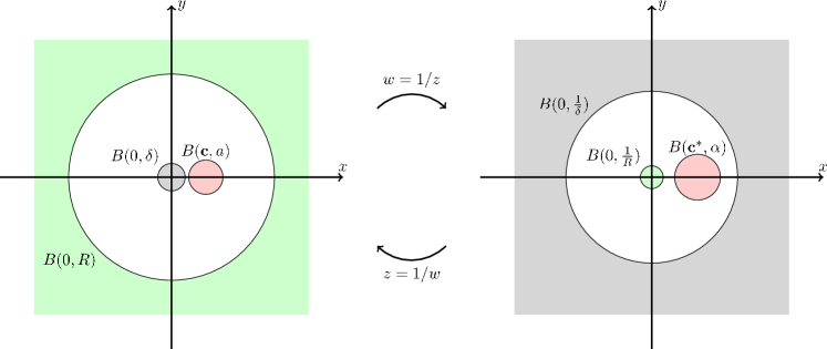
Figure 1: The effect of the inversion (Kelvin) transform $w=1/z$ on the cloak geometry. The cloaked region is in red and the device sources are all contained in the gray disk. The green region is the observation region, where the device field must be very small to avoid detection.

3 Cloak existence

The existence of a device field $u$ having the desired cloaking properties to within a tolerance $\epsilon$ is stated in the next theorem.

Theorem 3.1

Let $\epsilon>0$ be an arbitrarily small parameter. Let also $a>0$, ${\bf c}=(p,0)$, $p>0$ and $R$ satisfy the inequalities (1) and (2). Then for a harmonic incident field $u_{0}$, there are functions $g_{0}:\mathbb{R}^{2}\to\mathbb{R}$ and $u:\mathbb{R}^{2}\rightarrow\mathbb{R}$ such that

$$\left\{\begin{aligned} \Delta u&=0,~{}\text{in $\mathbb{R}^{2}\setminus\overline{B(0,\delta)}$},\\ u&=g_{0},~{}\text{on $\partial B(0,\delta)$},\\ \end{aligned}\right.$$ (3)

with $$|u|<\epsilon \mathbb{R}^{2}\setminus B(0,R) |u+u_{0}|<\epsilon B({\bf c},a)$$ in and in .

The main idea of the proof of Theorem 3.1 is to relate active exterior cloaking to the problem of approximating harmonic functions with harmonic polynomials. We rely on the following classic result.

Lemma 1 (Walsh, see e.g. Gardiner (1995), page 8)

Let $K$ be a compact set in $\mathbb{R}^{2}$ such that $\mathbb{R}^{2}\setminus K$ is connected. Then for each function $w$ harmonic on an open set containing $K$ and for any $\epsilon>0$, there is a harmonic polynomial $q$ for which $|w-q|<\epsilon$ on $K$.

We can now proceed with the proof of Theorem 3.1.

Proof

It is convenient to use complex numbers $z=x+iy$ to represent points $(x,y)\in\mathbb{R}^{2}$. By applying the inversion (Kelvin) transformation $w=1/z$, the geometry of the problem transforms as in Table 1. (see also Figure 1).

Region	$z$ plane	$w=1/z$ plane
Cloaking device	$B(0,\delta)$	$\mathbb{R}^{2}\setminus B(0,1/\delta)$
Cloaked region	$B({\bf c},a)$	$B({\bf c}^{*},\alpha)$ with ${\bf c}^{*}=(\beta,0)$, $\alpha=a/|p^{2}-a^{2}|$ and $\beta=p/(p^{2}-a^{2})$
Observation region	$\mathbb{R}^{2}\setminus B(0,R)$	$B(0,1/R)$

Table 1: The different regions in our cloak setup and how they are mapped by the inversion (Kelvin) transformation.

Thus the cloaking problem (3) is equivalent to finding functions $\widetilde{g}_{0}$ and $\widetilde{u}$ for which

$$\left\{\begin{aligned} \Delta\widetilde{u}&=0,~{}\text{in $B(0,1/\delta)$},\\ \widetilde{u}&=\widetilde{g}_{0},~{}\text{on $\partial B(0,1/\delta)$},\end{aligned}\right.$$ (4)

with $$|\widetilde{u}|<\epsilon \overline{B(0,1/R)} |\widetilde{u}+\widetilde{u}_{0}|<\epsilon B({\bf c}^{*},\alpha)$$ on and on .

Here $\epsilon$ is as in the statement of the theorem, $\widetilde{g}_{0}(z)=g_{0}(1/z)$ and the function $\widetilde{u}_{0}(z)=u_{0}(1/z)$ is harmonic on $\mathbb{R}^{2}\setminus\{0\}$.

Let $\widetilde{U}_{0}$ denote the analytic extension of $\widetilde{u}_{0}$ in $B({\bf c}^{*},\alpha)$, obtained by adding $i$ times its harmonic conjugate. Notice that since $\widetilde{U}_{0}$ is analytic, it can be arbitrarily well approximated by a polynomial, e.g. a truncation of the power series of $\widetilde{U}_{0}$. Therefore, there is a polynomial $Q_{0}$ such that

$$|\widetilde{U}_{0}-Q_{0}|<\epsilon/2,~{}~{}\text{on $\overline{B({\bf c}^{*},\alpha)}$}.$$ (5)

For $\widetilde{u}_{0}$ this means that

$$|\widetilde{u}_{0}-q_{0}|<\epsilon/2,~{}~{}\text{on $\overline{B({\bf c}^{*},\alpha)}$},$$ (6)

where $q_{0}$ is the real part of $Q_{0}$. Thus we may solve (4) by first approximating the (inverted) incident field $\widetilde{u}_{0}$ by $q_{0}$ and then studying the following problem

$$\left\{\begin{aligned} \Delta\widetilde{u}&=0,~{}\text{in $B(0,1/\delta)$},\\ \widetilde{u}&=\widetilde{g}_{0},~{}\text{on $\partial B(0,1/\delta)$},\end{aligned}\right.$$ (7)

with $$|\widetilde{u}|<\epsilon \overline{B(0,1/R)} |\widetilde{u}+q_{0}|<\epsilon/2 B({\bf c}^{*},\alpha)$$ on and on .

After inversion, the conditions (1) and (2) necessary for having an exterior cloak become

$$1/R <\beta-\alpha,~{}~{}\text{(the two disks $B(0,1/R)$ and $B({\bf c}^{*},\alpha)$ do not touch), and }$$ (8)

$$\beta+\alpha <1/\delta,~{}~{}\text{(the two disks $B(0,1/\delta)$ and $B({\bf c}^{*},\alpha)$ do not touch).}$$

Therefore, there exists $0<\xi\ll 1$ such that

$$\frac{1}{R}+\xi<\beta-\alpha-\xi.$$ (9)

We can now apply Lemma 1 to the compact set $K=\overline{B(0,1/R)}\cup\overline{B({\bf c}^{*},\alpha)}$ (which has a connected complement by virtue of (8)) and the function

$$w=\begin{cases}0&\text{in $B(0,\frac{1}{R}+\xi)$,}\\ -q_{0}&\text{in $B({\bf c}^{*},\alpha+\xi)$,}\end{cases}$$ (10)

which is a harmonic function in the open set $B(0,\frac{1}{R}+\xi)\cup B({\bf c}^{*},\alpha+\xi)$ (a set containing $K$). We obtain that there exists a harmonic polynomial $q$ such that $|q-w|<\epsilon/2$ on $K$. A solution to (7) is then given by $\widetilde{u}=q$ and $\widetilde{g}_{0}=q$ on $\partial B(0,1/\delta)$. This implies the statement of the theorem.

Remark 1

We assumed throughout this section that the incident field $u_{0}$ is harmonic on $\mathbb{R}^{2}$. This corresponds to a source located at infinity. Recall our method relies on approximating the Kelvin transformed analytic extension of the incident field $\widetilde{U}_{0}$ inside the Kelvin transformed cloaked region $B({\bf c}^{*},\alpha)$ by a polynomial $Q_{0}$ (see (11)). This approximation only requires analyticity of $U_{0}$ inside the cloaked region $B({\bf c},a)$. Hence the results of this section and the construction of Section 4 below generalize easily to the case where the incident field $u_{0}$ is harmonic inside the observation region $B(0,R)$. This is the case where the sources generating the incident field are outside the observation region but not necessarily located at infinity.

Remark 2

Clearly, Theorem 3.1 also holds when the device and cloaked region are not necessarily disks. The only requirements are that they be bounded, disjoint and that the complement of their union be connected (see Lemma 1).

4 A constructive solution for active cloaking

Although mathematically rigorous, the existence result of Theorem 3.1 does not give an explicit expression for the potential required at the active device (antenna). To give an explicit harmonic solution to problem (3), we first simplify the problem in Section 4.1. Then we give a candidate solution to the simplified problem in Section 4.2, in the form of a Lagrange interpolation polynomial. A better solution is constructed in Section 4.3 by averaging several Lagrange interpolation polynomials. The resulting polynomial turns out to be a Hermite interpolation polynomial. Then in Section 4.4 we show that this Hermite interpolation polynomial solves (4) (and thus the cloaking problem (3)) provided its degree is sufficiently large. This convergence study reveals constraints on the size of the cloaked region and the device that are due to the particular solution we construct.

4.1 Simplifying the problem

In the proof of Theorem 3.1, we related the cloaking problem (3) to the problem of approximating a polynomial $Q_{0}$ with an analytic function $V$ such that for some $\epsilon>0$,

$$|V|<\epsilon~{}\text{in $B(0,1/R)$ and}~{}|V+Q_{0}|<\epsilon~{}\text{in $B({\bf c}^{*},\alpha)$}.$$ (11)

Now consider the problem of finding an analytic function $W$ such that for some $\epsilon^{\prime}>0$,

$$|1-W|<\epsilon^{\prime}~{}\text{in $B(0,1/R)$ and}~{}|W|<\epsilon^{\prime}~{}\text{in $B({\bf c}^{*},\alpha)$}.$$ (12)

Assuming we can find an approximant $W$ in (12) with $\epsilon^{\prime}=\epsilon/M$ and

$$M=\sup_{z\in B({\bf c}^{*},\alpha)\cup B(0,1/R)}|Q_{0}(z)|,$$ (13)

a solution to (11) is then $V=-Q_{0}(1-W)$, which is analytic because the product of two analytic functions is analytic.

For illustration purposes we fast forward to Figure 3, where we give an example of a function $W$ with the approximation properties (12). The function $W$ is a polynomial whose motivation, derivation and analysis are the subject of the remainder of this section.

In order to use such a function $W$ for cloaking, assume $Q_{0}(1/z)$ is the harmonic incident field. Then the device field needed for solving the cloaking problem (3) is the real part of the function $U(1/z)=-Q_{0}(1/z)(1-W(1/z))$ (after having undone the Kelvin transformation we used for the analysis). The actual device field is illustrated in Figure 4. On the left, a scatterer perturbs the incident field and can be easily detected. On the right, the device field (based on the function $W$ of Figure 3 is activated and suppresses the incident field inside the cloaked region, making the object undetectable for all practical purposes.

4.2 A first candidate polynomial from Lagrange interpolation

Figure 2: Left: sample interpolation points for the interpolation polynomial $p_{\phi,\psi}$ with $n=5$, $\phi=0$ and $\psi=\pi/3$. Right: the modulus of the polynomial $p_{\phi,\psi}$ with $n=10$, $\phi=-\psi=\pi/10$ and $\beta=4$. The color scale is logarithmic and the interpolation nodes are indicated by the interpolation values.

We present a polynomial solution to (12) based on Lagrange interpolation. This is an intermediary step to motivate the explicit solution to (12) given later in Section 4.3. The idea applies only to the case where $\alpha=R=1$ and $\beta=p/(p^{2}-a^{2})>2$. The candidate solution is a polynomial that is one at $n$ equally distributed points on $\partial B(0,1)$ and zero at $n$ equally distributed points on $\partial B({\bf c}^{*},1)$. The motivation being that by surrounding both $0$ and ${\bf c}^{*}=(\beta,0)$ by $n$ points where the polynomial has the desired values, we hope to get close to a polynomial satisfying (12).

To be more precise, let us introduce the following family of $2n$ nodes $\{e^{i\phi}w_{j},\beta+e^{i\psi}w_{j}\}_{j=0}^{n-1}$. Here $\phi$ and $\psi$ are two arbitrary angles and $w_{j}=\exp[2i\pi j/n]$, for $j=0,\ldots,n-1$. Define the polynomial $p_{\phi,\psi}$ as the unique polynomial of degree $2n-1$ satisfying,

$$p_{\phi,\psi}(e^{i\phi}w_{j})=1~{}\text{and}~{}p_{\phi,\psi}(\beta+e^{i\psi}w_{j})=0,~{}\text{for $j=0,\ldots,n-1$.}$$ (14)

An example of the interpolation nodes and the values of $p_{\phi,\psi}$ is shown in Figure 2(left).

The polynomial $p_{\phi,\psi}$ is unique and can be written explicitly as

$$p_{\phi,\psi}(z)=\sum_{m=0}^{n-1}q_{\phi,\psi,m}(z),$$ (15)

where $q_{\phi,\psi,m}(z)$ are Lagrange interpolation polynomials (see e.g. Stoer and Bulirsch (2002)) defined for $m=0,\ldots,n-1$ by

$$q_{\phi,\psi,m}(z)=\left[{\prod_{j=0,j\neq m}^{n-1}\frac{z-e^{i\phi}w_{j}}{e^{i\phi}w_{m}-e^{i\phi}w_{j}}}\right]\left[{\prod_{j=0}^{n-1}\frac{z-(\beta+e^{i\psi}w_{j})}{e^{i\phi}w_{m}-(\beta+e^{i\psi}w_{j})}}\right],$$ (16)

or alternatively by their interpolation properties

$$q_{\phi,\psi,m}(e^{i\phi}w_{j})=\delta_{mj},~{}\text{and}~{}q_{\phi,\psi,m}(\beta+e^{i\psi}w_{j})=0,~{}\text{for $j=0,\ldots,n-1$}.$$ (17)

Here $\delta_{mj}=1$ if $m=j$ and $0$ otherwise is the Kronecker delta. Straightforward calculations give the expression

$$q_{\phi,\psi,m}(z)=\left[{\frac{(z-\beta)^{n}-e^{i\psi n}}{(e^{i\phi}w_{m}-\beta)^{n}-e^{i\psi n}}}\right]\left[{\frac{z^{n}-e^{i\phi n}}{z-e^{i\phi}w_{m}}}\right]\left[{\frac{1}{n(w_{m}e^{i\phi})^{n-1}}}\right],$$ (18)

which will be used later in Section 4.3.

We state the following symmetry property of the polynomial $p_{\phi,\psi}$ for later use.

Lemma 2

For any angles $\phi$ and $\psi$, the polynomial $p_{\phi,\psi}$ has the following symmetry property:

$$p_{\phi,\psi}(z)+p_{\psi+\pi,\phi+\pi}(\beta-z)=1.$$ (19)

Proof

Equation (19) follows from noticing that for $j=0,\ldots,n-1$,

$$p_{\psi+\pi,\phi+\pi}(\beta-(\beta+e^{i\psi}w_{j})) =p_{\psi+\pi,\phi+\pi}(e^{i(\psi+\pi)}w_{j})=0,~{}\text{and}$$ (20)

$$p_{\psi+\pi,\phi+\pi}(\beta-e^{i\phi}w_{j}) =p_{\psi+\pi,\phi+\pi}(\beta+e^{i(\phi+\pi)}w_{j})=1.$$

Hence the polynomial $p_{\phi,\psi}(z)+p_{\psi+\pi,\phi+\pi}(\beta-z)-1$ must be identically zero because it is of degree $2n-1$ and has $2n$ roots $\{e^{i\phi}w_{j},\beta+e^{i\psi}w_{j}\}_{j=0}^{n-1}$.

An actual polynomial $p_{\phi,\psi}$ is shown in Figure 2(right). Unfortunately this polynomial is not a good solution for problem (12) as the regions where $p_{\phi,\psi}\approx 1$ and $p_{\phi,\psi}\approx 0$ to within a certain tolerance (say 1%) are relatively small. Changing $\phi$ and $\psi$ does not give a significant improvement. However these polynomials are the building block for the ensemble average polynomial solving (12) that we present next.

4.3 The ensemble average polynomial

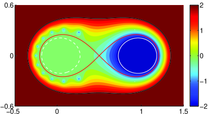
Figure 3: The modulus of the ensemble average polynomial $\left\langle{p}\right\rangle(z)$ for $n=12$ and $\beta=1$. The device field used for cloaking is $\left\langle{p}\right\rangle(1/z)$. Within 1% accuracy, the polynomial $\left\langle{p}\right\rangle$ is close to one inside the dashed white circle and close to zero inside the solid white circle. The boundary of the convergence region $D_{\beta}$ of $\left\langle{p}\right\rangle$ as $n\to\infty$ is the peanut shaped curve in red (see Theorem 4.1). The color scale is logarithmic from $0.01$ (dark blue) to $100$ (dark red), with light green representing 1.

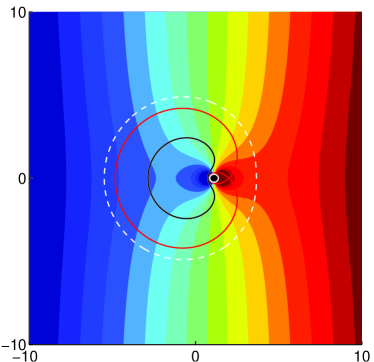
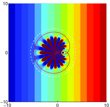
Figure 4: Real part of the total field with the cloaking device active (right) and inactive (left), for an incident field $u_{0}(z)=z$ and $n=12$. The solid white, dashed white and red curves are the Kelvin transforms of the respective curves in Figure 3. The solid black disk is an almost resonant scatterer with radius $r=0.1$, located at $z=1.05$ and with dielectric constant $\epsilon=-1+10^{-3}$, chosen to be plasmonic with a negative value close to $-1$ to amplify its effect. The solid black curve is the contour $|u|=100$. The color scale is linear from -10 (dark blue) to 10 (dark red).

In an effort to obtain a polynomial solution to problem (12) we calculate the ensemble average of the polynomials $p_{\phi,\psi}$ with respect to the two phase factors $\phi,\psi\in[0,2\pi]$, that is

$$\left\langle{p}\right\rangle(z)=\frac{1}{(2\pi)^{2}}\int_{0}^{2\pi}\int_{0}^{2\pi}p_{\phi,\psi}(z)d\phi d\psi.$$ (21)

We prove in Theorem 4.1, using the next lemma, that indeed $\left\langle{p}\right\rangle$ is a solution for (12). An example of such polynomial for $\beta=1$ and $n=12$ is given in Figure 3.

Lemma 3

The ensemble average polynomial defined in (21) has the expression

$$\left\langle{p}\right\rangle(z)=\left({1-\frac{z}{\beta}}\right)^{n}\,\sum_{j=0}^{n-1}\left({\frac{z}{\beta}}\right)^{j}\frac{(n+j-1)!}{j!(n-1)!}.$$ (22)

Proof

We first use the Cauchy residue theorem to compute the integral

$$\frac{1}{2\pi}\int_{0}^{2\pi}\frac{(z-\beta)^{n}-e^{i\psi n}}{(e^{i\phi}w_{m}-\beta)^{n}-e^{i\psi n}}d\psi =\frac{1}{2i\pi}\int_{|w|=1}\frac{(z-\beta)^{n}-w^{n}}{(e^{i\phi}w_{m}-\beta)^{n}-w^{n}}\frac{dw}{w}$$ (23)

$$=\frac{(z-\beta)^{n}}{(e^{i\phi}w_{m}-\beta)^{n}},$$

since the integrand has a single simple pole at $w=0$ in the disk $|w|<1$. Then by plugging (23) into the expression for $q_{\phi,\psi,m}$ we get that

$$\frac{1}{2\pi}\int_{0}^{2\pi}q_{\phi,\psi,m}(z)d\psi=\frac{(z-\beta)^{n}}{(e^{i\phi}w_{m}-\beta)^{n}}\frac{z^{n}-e^{i\phi n}}{z-e^{i\phi}w_{m}}\frac{1}{n(w_{m}e^{i\phi})^{n-1}}.$$ (24)

Recalling that $p_{\phi,\psi}$ is the sum (15) of $q_{\phi,\psi,m}$ we can write

$$\left\langle{p}\right\rangle(z)=\frac{1}{2\pi}\sum_{m=0}^{n-1}\frac{(z-\beta)^{n}}{(e^{i\phi}w_{m}-\beta)^{n}}\frac{z^{n}-e^{i\phi n}}{z-e^{i\phi}w_{m}}\frac{1}{n(w_{m}e^{i\phi})^{n-1}}.$$ (25)

Now all $n$ terms in the previous sum are identical, therefore

$$\left\langle{p}\right\rangle(z) =\frac{1}{2\pi}\int_{0}^{2\pi}\frac{(z-\beta)^{n}}{(e^{i\phi}-\beta)^{n}}\frac{z^{n}-e^{i\phi n}}{z-e^{i\phi}}\frac{1}{e^{i\phi(n-1)}}$$ (26)

$$=\frac{1}{2i\pi}\int_{|w|=1}(z-\beta)^{n}\frac{z^{n}-w^{n}}{(z-w)(w-\beta)^{n}}\frac{dw}{w^{n}}$$

$$=\frac{(z-\beta)^{n}}{2i\pi}\int_{|w|=1}\left({\frac{z^{n}}{w^{n}}-1}\right)\frac{1}{(z-w)(w-\beta)^{n}}dw$$

$$=\frac{(z-\beta)^{n}}{2i\pi}\int_{|w|=1}\sum_{j=0}^{n-1}\frac{z^{j}}{w^{j+1}(w-\beta)^{n}}dw$$

$$=(z-\beta)^{n}\sum_{j=0}^{n-1}\frac{z^{j}}{j!}\frac{d^{j}}{dw^{j}}\left[{\frac{1}{(w-\beta)^{n}}}\right]_{w=0},$$

where we used Cauchy’s theorem in the last equality of (26). The desired expression (22) follows by straightforward algebraic manipulations of (26).

Remark 3

By using elementary algebraic manipulations and (26), it is possible to show that $\left\langle{p}\right\rangle$ is the Hermite interpolation polynomial Stoer and Bulirsch (2002) of degree $2n-1$ that is uniquely defined by the $2n$ interpolation conditions

$$\left\langle{p}\right\rangle(0)=1,~{}\left\langle{p}\right\rangle(\beta)=0,~{}\text{and}~{}\left\langle{p}\right\rangle^{(j)}(0)=\left\langle{p}\right\rangle^{(j)}(\beta)=0,~{}\text{for $j=1,\ldots,n-1$.}$$ (27)

Notice that the ensemble average polynomial inherits the symmetry property (19) for $p_{\phi,\psi}$, that is

$$\left\langle{p}\right\rangle(z)+\left\langle{p}\right\rangle(\beta-z)=1.$$ (28)

This symmetry property means that by design, the polynomial gives as good an approximation to one near the origin as the approximation to zero near $\beta$.

4.4 Asymptotics of the ensemble average polynomial

We now study the behavior of the polynomial $\left\langle{p}\right\rangle$ (defined in (21)) as $n\to\infty$. The following result shows that the polynomial $\left\langle{p}\right\rangle$ solves the problem (12), and gives limits to the size of the cloaked region.

Theorem 4.1

The ensemble average polynomial $\left\langle{p}\right\rangle$ can be written as

$$\left\langle{p}\right\rangle=\frac{1}{2}+\sum_{k=0}^{n-1}\frac{(2k)!}{(k!)^{2}}\left({\frac{z}{\beta}\left({1-\frac{z}{\beta}}\right)}\right)^{k}\left({\frac{1}{2}-\frac{z}{\beta}}\right).$$ (29)

The polynomial $\left\langle{p}\right\rangle(z)$ converges as $n\to\infty$ if and only if $z$ belongs to the convergence region

$$D_{\beta}=\left\{{z\in\mathbb{C},~{}|z^{2}-\beta z|<\frac{\beta^{2}}{4}}\right\}.$$ (30)

The convergence is uniform on compact subsets of $D_{\beta}$ to the function

$$\chi(z)=\begin{cases}1&\text{if}\;\;\Re(z)<\beta/2,\\ 0&\text{otherwise.}\end{cases}$$ (31)

For large enough $n$, the polynomial $\left\langle{p}\right\rangle$ solves (12) if and only if

$$\frac{1}{R}<\frac{\beta}{2\sqrt{2}+2}~{}~{}~{}\text{and}~{}~{}~{}\alpha<\frac{\beta}{2\sqrt{2}+2}.$$ (32)

Proof

Consider the function

$$f_{n}(t)=(1-t)^{n}\sum_{j=0}^{n-1}t^{j}{n+j-1\choose j}$$ (33)

where for any positive integers $m$ and $p$, ${m\choose p}=\frac{m!}{p!(m-p)!}$. Note that, from (22) we have

$$f_{n}(t)=\left\langle{p}\right\rangle(\beta t),\mbox{ for all }t\in\mathbb{C}.$$ (34)

Then for all $t\neq 1$ we obtain,

$$\frac{f_{n+1}(t)}{(1-t)^{n+1}} =\sum_{j=0}^{n}t^{j}{n+j\choose j}$$ (35)

$$=1+\sum_{j=1}^{n}t^{j}\left[{n+j-1\choose j-1}+{n+j-1\choose j}\right]$$

$$=\sum_{j=1}^{n}t^{j}{n+j-1\choose j-1}+\left[1+\sum_{j=1}^{n}t^{j}{n+j-1\choose j}\right]$$

$$=\sum_{k=0}^{n-1}t^{k+1}{n+k\choose k}+\sum_{j=0}^{n}t^{j}{n+j-1\choose j}$$

$$=t\left[\frac{f_{n+1}(t)}{(1-t)^{n+1}}-t^{n}{2n\choose n}\right]+\frac{f_{n}(t)}{(1-t)^{n}}+t^{n}{2n-1\choose n}.$$

In the above equation we used the recurrence relation

$${m\choose p}={m-1\choose p-1}+{m-1\choose p},\mbox{ for any integers }m,p>0.$$

From (35), for any integer $n\geq 1$ we obtain,

$$f_{n+1}(t) =f_{n}(t)-(1-t)^{n}t^{n+1}{2n\choose n}+(1-t)^{n}t^{n}{2n-1\choose n}$$ (36)

$$=f_{n}(t)-(1-t)^{n}t^{n}{2n\choose n}\left({t-\frac{1}{2}}\right),\;\;\mbox{ for all }t\neq 1.$$

In (36) we used the identity

$${2n\choose n}=2{2n-1\choose n},\mbox{ for every integer }n\geq 1.$$

From the first order linear recurrence (36) we obtain,

$$f_{n}(t)=\frac{1}{2}+\sum_{k=0}^{n-1}(1-t)^{k}t^{k}{2k\choose k}\left(\frac{1}{2}-t\right)$$ (37)

and this is valid for all $n\geq 1$ and all $t\in\mathbb{C}$ (as (37) which was initially obtained for $t\neq 1$ checks also for $t=1$). The final expression (29) follows from substituting $t=z/\beta$ in (37) and using (34).

Notice that the polynomial $\left\langle{p}\right\rangle$ is in fact the $n$-th order partial sum of the following infinite sum,

$$\frac{1}{2}+\sum_{k=0}^{\infty}(1-\frac{z}{\beta})^{k}\left(\frac{z}{\beta}\right)^{k}{2k\choose k}\left(\frac{1}{2}-\frac{z}{\beta}\right).$$

By the ratio test this series converges uniformly on compacts subsets of the region $D_{\beta}$ (defined at (30)) to a limit function $\varphi$ and diverges in $\mathbb{C}\setminus{\overline{D}_{\beta}}$. From the uniform convergence of $\left\langle{p}\right\rangle$ we deduce the analyticity of $\varphi$ in $D_{\beta}$ and by using the Taylor expansion around the origin for $\varphi$, the Remark 3, and the symmetry property (28) we obtain convergence to the function (31) inside $D_{\beta}$.

We now study the convergence region $D_{\beta}$ in order to show that the constraints (32) are necessary and sufficient for $\left\langle{p}\right\rangle$ to solve (12). First notice that the definition of the region $D_{\beta}$ and simple algebra reveal that

$$\frac{1}{R}<\frac{\beta}{2\sqrt{2}+2} \Leftrightarrow \frac{1}{R}e^{-i\pi}\in(D_{\beta}\cap\{z\in{\mathbb{C}},2Re(z)<\beta\}),~{}\text{and}$$ (38)

$$\alpha<\frac{\beta}{2\sqrt{2}+2} \Leftrightarrow \beta+\alpha\in(D_{\beta}\cap\{z\in{\mathbb{C}},2Re(z)>\beta\}).$$ (39)

Next we show that

$$\frac{1}{R}<\frac{\beta}{2\sqrt{2}+2} \Leftrightarrow B(0,1/R)\Subset(D_{\beta}\cap\{z\in{\mathbb{C}},\;2Re(z)<\beta\}),~{}\text{and}$$ (40)

$$\alpha<\frac{\beta}{2\sqrt{2}+2} \Leftrightarrow B({\bf c}^{*},\alpha)\Subset(D_{\beta}\cap\{z\in{\mathbb{C}},\;2Re(z)>\beta\}),$$ (41)

where $\Subset$ is the classical symbol for compact inclusions. By using the equivalences (38) and (39) it is easy to check that the inclusions in (40) and (41) imply the constraints (32). To show the implication ($\Rightarrow$), we first show that for any two positive real numbers $l,q$ with $2\max\{l,q\}<\beta$, we have

$$le^{-\pi i}\in D_{\beta} \Leftrightarrow \overline{B(0,l)}\Subset(D_{\beta}\cap\{z\in\mathbb{C},2Re(z)<\beta\})~{}\text{and}$$ (42)

$$\beta+q\in D_{\beta} \Leftrightarrow \overline{B({\bf c}^{*},q)}\Subset(D_{\beta}\cap\{z\in\mathbb{C},2Re(z)>\beta\}).$$ (43)

Let us first show the equivalence (42). The sufficiency ($\Leftarrow$) is immediate. For the other implication ($\Rightarrow$), we can use the definition of $D_{\beta}$ to show that for any $\theta\in[-\pi,\pi]$ we have,

$$le^{i\theta}\in D_{\beta} \Leftrightarrow |l^{2}e^{i\theta}-\beta l|<\frac{\beta^{2}}{4}$$ (44)

$$\Leftrightarrow (l^{2}e^{i\theta}-\beta l)(l^{2}e^{-i\theta}-\beta l)<\frac{\beta^{4}}{16}$$

$$\Leftrightarrow l^{4}+\beta^{2}l^{2}-2l^{3}\beta\cos\theta-\frac{\beta^{4}}{16}<0.$$

Since we assumed $le^{-\pi i}\in D_{\beta}$, equation (44) immediately implies that

$$l^{4}+\beta^{2}l^{2}+2l^{3}\beta-\frac{\beta^{4}}{16}<0.$$ (45)

Consider the even function $f:[-\pi,\pi]\rightarrow\mathbb{R}$ defined by,

$$f(\theta)=l^{4}+\beta^{2}l^{2}-2l^{3}\beta\cos\theta-\frac{\beta^{4}}{16}.$$ (46)

Observe now that, because $l>0$, its derivative $f^{\prime}(\theta)=2l^{3}\beta\sin\theta$ has the signs,

$$f^{\prime}(\theta)\geq 0~{}\text{for $\theta\in[0,\pi]$}~{}~{}\text{and}~{}~{}~{}f^{\prime}(\theta)\leq 0~{}\text{for $\theta\in[-\pi,0]$}.$$ (47)

Note that from inequality (45) and the definition (46) of $f(\theta)$ one immediately obtains

$$f(-\pi)=f(\pi)<0.$$ (48)

Then the signs of $f^{\prime}(\theta)$ in (47) together with the particular values of $f(\theta)$ in (48) imply

$$f(\theta)<\max\{f(\pi),f(-\pi)\}<0,\mbox{ for all }\theta\in[-\pi,\pi].$$ (49)

Because of equivalence (44) we conclude from inequality (49) that

$$le^{i\theta}\in D_{\beta},\mbox{ for any }\theta\in[-\pi,\pi].$$ (50)

From the conditions on $l$, we have that $2Re(le^{i\theta})\leq 2l<\beta$ and by using this in (50) we obtain

$$le^{i\theta}\in(D_{\beta}\cap\{z\in\mathbb{C},2Re(z)<\beta\}),\mbox{ for any }\theta\in[-\pi,\pi].$$ (51)

Inclusion (51) together with the convexity of $D_{\beta}\cap\{z\in\mathbb{C},2Re(z)<\beta\}$ implies that

$${\overline{B}}_{l}(0)\Subset D_{\beta}\cap\{z\in{\mathbb{C}},2Re(z)<\beta\}.$$

This establishes the equivalence (42). From the definition of the set $D_{\beta}$, by simple algebraic manipulation we obtain

$$\beta+q\in D_{\beta}\Leftrightarrow qe^{-\pi i}\in D_{\beta}.$$ (52)

Equivalence (52) clearly implies that (43) follows from (42) applied to $q$ instead of $l$. Finally, observing the fact that the constraints (32) imply $2\max\{\frac{1}{R},\alpha\}<\beta$ and using equivalences (38), (39), (42) and (43) for $\frac{1}{R}$ and $\alpha$ instead of $l$ and $q$ respectively, we obtain the desired equivalences (40) and (41). By using the uniform convergence of the polynomial $\left\langle{p}\right\rangle$ to the function $\chi(z)$ in $D_{\beta}$, and equivalences (40) and (41) we obtain that the constraints (32) are indeed necessary and sufficient for convergence of $\left\langle{p}\right\rangle$.

Remark 4

The expression (29) of the ensemble average polynomial could also be obtained by generalizing to distributions a theorem by Ramharter Ramharter (1991) (which is in turn a generalization of a result due to Berger and Tasche Berger and Tasche (1988)). To remain concise, we prefer to include a direct proof.

5 Summary

For the Laplace equation we have shown the existence of a device capable of cloaking a region exterior to the device, assuming a priori knowledge of the incident field. The proof relies on a non-constructive harmonic function approximation result. The theory does not constrain the size and relative positions of the device and cloaked region, as long as they are bounded, disjoint and the complement of their union is connected. Although the construction of such a cloaking device is clearly not unique, we presented earlier in Guevara Vasquez et al. (2009a) a construction based on an explicit polynomial. Here we rigorously justify this construction and show that the constraints (32) must be satisfied in order to have a proper active exterior cloak. Because of the constraints (32), the current strategy fails to cloak large objects ($\alpha$ large) unless they are sufficiently far from the origin ($\beta$ large enough). In Guevara Vasquez et al. (2011b) (see Conjecture 1), we present without proof, as a conjecture, an extension of Theorem 4.1 which gives a wider choice of cloaks and that is supported by numerical experiments.

References

• Alú and Engheta [2008] A. Alú and N. Engheta. Plasmonic and metamaterial cloaking: physical mechanisms and potentials. J. Opt. A: Pure Appl. Opt., 10:093002, 2008.
• Berger and Tasche [1988] G. Berger and M. Tasche. Hermite-Lagrange interpolation and Schur’s expansion of ${\rm sin}\,\pi x$. J. Approx. Theory, 53(1):17–25, 1988. ISSN 0021-9045. doi: 10.1016/0021-9045(88)90072-X.
• Chen and Chan [2007] H. Chen and C. T. Chan. Acoustic cloaking in three dimensions using acoustic metamaterials. Appl. Phys. Lett., 91:183518, 2007.
• Dolin [1961] L. S. Dolin. To the possibility of comparison of three-dimensional electromagnetic systems with nonuniform anisotropic filling. Izv. Vyssh. Uchebn. Zaved. Radiofizika, 4(5):964–967, 1961.
• Gardiner [1995] S. J. Gardiner. Harmonic approximation, volume 221 of London Mathematical Society Lecture Note Series. Cambridge University Press, Cambridge, 1995. ISBN 0-521-49799-X. doi: 10.1017/CBO9780511526220.
• Greenleaf et al. [2003] A. Greenleaf, M. Lassas, and G. Uhlmann. Anisotropic conductivities that cannot be detected by EIT. Physiological Measurement, 24:413–419, 2003.
• Greenleaf et al. [2009] A. Greenleaf, Y. Kurylev, M. Lassas, and G. Uhlmann. Invisibility and inverse problems. Bull. Amer. Math. Soc. (N.S.), 46(1):55–97, 2009. ISSN 0273-0979. doi: 10.1090/S0273-0979-08-01232-9.
• Guevara Vasquez et al. [2009a] F. Guevara Vasquez, G. W. Milton, and D. Onofrei. Active exterior cloaking for the 2D Laplace and Helmholtz equations. Phys. Rev. Lett., 103:073901, 2009a. doi: 10.1103/PhysRevLett.103.073901.
• Guevara Vasquez et al. [2009b] F. Guevara Vasquez, G. W. Milton, and D. Onofrei. Broadband exterior cloaking. Opt. Express, 17:14800–14805, 2009b. doi: 10.1364/OE.17.014800.
• Guevara Vasquez et al. [2011a] F. Guevara Vasquez, G. W. Milton, and D. Onofrei. Exterior cloaking with active sources in two dimensional acoustics. Wave Motion, 48(6):515 – 524, 2011a. ISSN 0165-2125. doi: 10.1016/j.wavemoti.2011.03.005. Special Issue on Cloaking of Wave Motion.
• Guevara Vasquez et al. [2011b] F. Guevara Vasquez, G. W. Milton, D. Onofrei, and P. Seppecher. Transformation elastodynamics and active exterior acoustic cloaking. In S. Guenneau and R. Craster, editors, Acoustic Metamaterials: Negative refraction, imaging, lensing and cloaking. Springer, 2011b. Submitted for publication. arXiv:1105.1221.
• Kohn et al. [2010] R. V. Kohn, D. Onofrei, M. S. Vogelius, and M. I. Weinstein. Cloaking via change of variables for the Helmholtz equation. Comm. Pure Appl. Math., 63(8):973–1016, 2010. ISSN 0010-3640.
• Lai et al. [2009] Y. Lai, H. Chen, Z.-Q. Zhang, and C. T. Chan. Complementary media invisibility cloak that cloaks objects at a distance outside the cloaking shell. Phys. Rev. Lett., 102:093901, 2009.
• Leonhardt [2006a] U. Leonhardt. Notes on conformal invisibility devices. New Journal of Physics, 8:118, 2006a.
• Leonhardt [2006b] U. Leonhardt. Optical conformal mapping. Science, 312:1777–1780, 2006b.
• Miller [2006] D. A. B. Miller. On perfect cloaking. Opt. Express, 14:12457–12466, 2006.
• Milton and Nicorovici [2006] G. W. Milton and N.-A. P. Nicorovici. On the cloaking effects associated with anomalous localized resonance. Proc. R. Soc. Lon. Ser. A. Math. Phys. Sci., 462:3027–3059, 2006. ISSN 0080-4630.
• Milton et al. [2008] G. W. Milton, N.-A. P. Nicorovici, R. C. McPhedran, K. Cherednichenko, and Z. Jacob. Solutions in folded geometries, and associated cloaking due to anomalous resonance. New J. Phys., 10:115021, 2008.
• Nicorovici et al. [2007] N.-A. P. Nicorovici, G. W. Milton, R. C. McPhedran, and L. C. Botten. Quasistatic cloaking of two-dimensional polarizable discrete systems by anomalous resonance. Opt. Express, 15:6314–6323, 2007.
• Pendry et al. [2006] J. B. Pendry, D. Schurig, and D. R. Smith. Controlling electromagnetic fields. Science, 312(5781):1780–1782, 2006.
• Ramharter [1991] G. Ramharter. A remark on Hermite-Lagrange interpolation. J. Approx. Theory, 66(1):109–113, 1991. ISSN 0021-9045. doi: 10.1016/0021-9045(91)90061-E.
• Silveirinha et al. [2008] M. G. Silveirinha, A. Alù, and N. Engheta. Cloaking mechanism with antiphase plasmonic satellites. Phys. Rev. B, 78(20):205109, Nov 2008. doi: 10.1103/PhysRevB.78.205109.
• Smolyaninov et al. [2009] I. I. Smolyaninov, V. N. Smolyaninova, A. V. Kildishev, and V. M. Shalaev. Anisotropic metamaterials emulated by tapered waveguides: Application to optical cloaking. Phys. Rev. Lett., 102:213901, 2009.
• Stoer and Bulirsch [2002] J. Stoer and R. Bulirsch. Introduction to numerical analysis, volume 12 of Texts in Applied Mathematics. Springer-Verlag, New York, third edition, 2002. ISBN 0-387-95452-X. Translated from the German by R. Bartels, W. Gautschi and C. Witzgall.