Testing Scaling Relations for Solar-Like Oscillations from the Main Sequence to Red Giants using Kepler Data

Abstract

We have analyzed solar-like oscillations in $\sim$1700 stars observed by the Kepler Mission, spanning from the main-sequence to the red clump. Using evolutionary models, we test asteroseismic scaling relations for the frequency of maximum power ($\nu_{\rm max}$), the large frequency separation ($\Delta\nu$) and oscillation amplitudes. We show that the difference of the $\Delta\nu$-$\nu_{\rm max}$ relation for unevolved and evolved stars can be explained by different distributions in effective temperature and stellar mass, in agreement with what is expected from scaling relations. For oscillation amplitudes, we show that neither $(L/M)^{s}$ scaling nor the revised scaling relation by Kjeldsen & Bedding (2011) is accurate for red-giant stars, and demonstrate that a revised scaling relation with a separate luminosity-mass dependence can be used to calculate amplitudes from the main-sequence to red-giants to a precision of $\sim$25%. The residuals show an offset particularly for unevolved stars, suggesting that an additional physical dependency is necessary to fully reproduce the observed amplitudes. We investigate correlations between amplitudes and stellar activity, and find evidence that the effect of amplitude suppression is most pronounced for subgiant stars. Finally, we test the location of the cool edge of the instability strip in the Hertzsprung-Russell diagram using solar-like oscillations and find the detections in the hottest stars compatible with a domain of hybrid stochastically excited and opacity driven pulsation.

1. Introduction

Empirical relations connecting observable quantities with physical parameters of stars are of fundamental importance for many fields of stellar astrophysics, with classical examples including the colour-temperature scale for late-type stars (see, e.g., Flower, 1996; Casagrande et al., 2010) and the period-luminosity relation for Cepheid variables (Leavitt, 1908). The calibration of these relations relies either on the direct measurement of stellar properties (e.g. through trigonometric parallaxes and interferometry) or the comparison of observations with stellar models. In both cases measurements spanning an extended range in parameter space (such as temperature, luminosity and metallicity) are required.

One of the most powerful methods to constrain fundamental properties of field stars is asteroseismology (see, e.g., Brown & Gilliland, 1994; Christensen-Dalsgaard, 2004; Aerts et al., 2010). The connection of global asteroseismic observables to fundamental stellar properties was calibrated by Kjeldsen & Bedding (1995, hereafter KB95) by introducing relations that scale stellar properties from the observed values of the Sun. The scaling relations have been used extensively both for the direct inference of stellar properties (e.g., Stello et al., 2009b; Kallinger et al., 2010a; Mosser et al., 2010; Kallinger et al., 2010b; Chaplin et al., 2011a; Hekker et al., 2011b, a; Silva Aguirre et al., 2011) as well as for calculating pulsation amplitudes of main-sequence and subgiant stars (e.g., Michel et al., 2008; Bonanno et al., 2008; Mathur et al., 2010b; Huber et al., 2011; Chaplin et al., 2011c) and red-giant stars (Edmonds & Gilliland, 1996; Gilliland, 2008; Stello & Gilliland, 2009; Mosser et al., 2010; Huber et al., 2010; Baudin et al., 2011; Stello et al., 2011). The three global observables discussed in this paper are the frequency of maximum power ($\nu_{\rm max}$), the large frequency separation ($\Delta\nu$) and the mean oscillation amplitude per radial mode.

Tests of the scaling relations for these observables over a wide range of parameter space has so far been hampered by the relative sparsity of detections of solar-like oscillations. The success of the Kepler mission has changed this picture, with the detection of oscillations in thousands of stars covering a large part of the low-mass region in the H-R diagram (Gilliland et al., 2010b). In this paper, we aim to use the large number of detections by Kepler to test scaling relations for stars ranging from the main-sequence to He-core burning red-giants.

2. Data Analysis and Models

The Kepler space telescope was launched in March 2009 with the primary goal of finding Earth-like planets orbiting solar-like stars through the detection of photometric transits. Kepler monitors the brightness of stars at two sampling rates, either in 29.4 min (long cadence) or in 58.8 sec (short cadence) intervals (Gilliland et al., 2010a; Jenkins et al., 2010). For asteroseismic studies of solar-like oscillators, the former are primarily used to study oscillations in red-giant stars, and short cadence data are used to measure the more rapid oscillations in main-sequence and subgiant stars. While red giants observed in long cadence have been continuously monitored since the launch of the mission, the number of short cadence slots is restricted due to bandwidth limitations. Short cadence slots have therefore so far been primarily used to survey a large number of stars for a period of one month each.

Kepler observations are subdivided into quarters, starting with the initial commissioning run (10 d, Q0), followed by a short first quarter (34 d, Q1) and subsequent full quarters of 90 d length. Our studies are based on Kepler data spanning from Q0 to Q6 for long cadence data and Q0 to Q4 for short cadence data. Our final sample contains 1686 stars, of which 1144 have been observed at long cadence, mostly since the launch of the mission ($\sim\,500$ days), and 542 at short cadence for a typical length of one month. We have used Kepler raw data, which were reduced in the manner described by García et al. (2011) and analyzed using several automated analysis methods (Bonanno et al., 2008; Campante et al., 2010; Hekker et al., 2010b; Huber et al., 2009; Kallinger et al., 2010a; Karoff et al., 2010; Mathur et al., 2010a; Mosser & Appourchaux, 2009; Mosser et al., 2011b; Verner & Roxburgh, 2011). We refer the reader to Hekker et al. (2011c) and Verner et al. (2011a) for an extensive comparison of the results provided by these methods. Unless otherwise mentioned, all results presented here are based on the method by Huber et al. (2009). We have only retained results for stars with at least one matching pipeline result within 10% and 5% of the determined $\nu_{\rm max}$ and $\Delta\nu$ value, respectively. The same outlier rejection procedure was repeated for all methods that returned results for both long cadence and short cadence data, and these datasets have then been used to validate all results and conclusions reported in this paper. Note that all amplitudes shown in this paper have been normalized to recover the full sine-amplitude of an injected signal (commonly referred to as peak-scaling). All amplitudes shown have been calculated using the method described by Kjeldsen et al. (2008) with $c=3.04$ (Bedding et al., 2010) to convert to amplitude per radial mode.

Uncertainties on $\nu_{\rm max}$, $\Delta\nu$ and amplitudes reported in this paper were estimated using Monte-Carlo simulations by generating synthetic power spectra following a $\chi^{2}$ distribution with two degrees of freedom with expected values corresponding to the observed power density levels. For each star, the method by Huber et al. (2009) was repeated on each synthetic dataset and the standard deviation of the distribution after 500 iterations was taken as an estimate of the uncertainty. The typical relative uncertainties obtained using this method for long cadence and short cadence data are 3% and 4% for $\nu_{\rm max}$, 1% and 3% for $\Delta\nu$, and 7% and 11% for the amplitude. These estimates agree with the results obtained by Hekker et al. (2011c) and Verner et al. (2011a). For our analysis, only stars with uncertainties lower than 20% in $\nu_{\rm max}$, 10% in $\Delta\nu$ and 50% in amplitude were retained. Note that oscillation amplitudes for all stars observed in long-cadence with $\mbox{$\nu_{\rm max}$}>200\mbox{$\mu$Hz}$ have been removed from our analysis due to the difficulty of estimating the noise level close to the Nyquist frequency of 283$\mu$Hz.

The asteroseismic relations discussed in this paper rely on scaling from observed values of the Sun. To ensure that these reference values are consistent with our analysis method, we used 111 30-day subsets of data collected by the VIRGO instrument (Fröhlich et al., 1997) aboard the SOHO spacecraft spanning from 1996 to 2005 and analyzed them in the same way as the Kepler data. This yielded solar reference values of $\nu_{\rm max,\sun}=3090\pm 30\mbox{$\mu$Hz}$ and $\Delta\nu_{\sun}=135.1\pm 0.1\mbox{$\mu$Hz}$, which are consistent with previously quoted values in the literature. We determined the oscillation amplitude to be $A_{\sun}=4.4\pm 0.3$ ppm for the VIRGO green channel ($\lambda=500$ nm) which, using the approximation by KB95, translates into a solar bolometric amplitude of $A_{\sun,\rm bol}=3.5\pm 0.2$ ppm. This is in excellent agreement with the solar reference value of 3.6 ppm established by Michel et al. (2009), and we have adopted $A_{\sun,\rm bol}=3.6$ ppm for the remainder of this paper.

In the absence of directly determined fundamental properties for most of the Kepler stars, a test of asteroseismic scaling relations relies on the comparison of observations with models. In our study, we use canonical BaSTI evolutionary models (Pietrinferni et al., 2004) with a solar-scaled distribution of heavy elements (Grevesse & Noels, 1993). Mass loss in BaSTI models is characterized according to the Reimers law (Reimers, 1975), and we used models with the mass loss parameter set to the commonly used value $\eta=0.4$ (see, e.g., Fusi-Pecci & Renzini, 1976). Note that mass loss for these models is only significant in the red giant phase of stellar evolution.

3. Scaling relations for $\nu_{\rm max}$ and $\Delta\nu$

Brown et al. (1991) first argued that the frequency of maximum power ($\nu_{\rm max}$) for Sun-like stars should scale with the acoustic cut-off frequency. KB95 used this assumption to relate $\nu_{\rm max}$ to stellar properties as follows:

$$\nu_{\rm max}\approx\frac{M/M_{\sun}(T_{\rm eff}/T_{\rm eff,\sun})^{3.5}}{L/L_{\sun}}\nu_{\rm max,\sun}\>.$$ (1)

This scaling relation has since been found to work well both observationally (see, e.g., Bedding & Kjeldsen, 2003; Stello et al., 2008; Bedding, 2011) as well as theoretically (see, e.g., Chaplin et al., 2008; Belkacem et al., 2011).

The mean large frequency separation ($\Delta\nu$) between modes of consecutive radial overtone and equal spherical degree is directly related to the sound travel time across the stellar diameter, and is therefore sensitive to the mean stellar density (Ulrich, 1986). This is expressed in the following scaling relation:

$$\Delta\nu\approx\frac{(M/M_{\sun})^{0.5}(T_{\rm eff}/T_{\rm eff,\sun})^{3}}{(L/L_{\sun})^{0.75}}\Delta\nu_{\sun}\>.$$ (2)

Note that in our analysis $\Delta\nu$ is measured as the mean spacing of all detectable modes around the value of $\nu_{\rm max}$ in the power spectrum.

Figure 1.— Upper panel: $\Delta\nu$ versus $\nu_{\rm max}$ for the entire sample of Kepler stars. Red triangles show stars observed in long cadence, while black diamonds are stars observed in short cadence. Lower panel: Same as upper panel, but with the luminosity dependence removed by raising $\nu_{\rm max}$ to the power of 0.75. Green lines show power law fits to the $\Delta\nu$-$\nu_{\rm max}$ relation for two different intervals of $\nu_{\rm max}$ (see text). The blue dashed line shows the relation by Stello et al. (2009a).

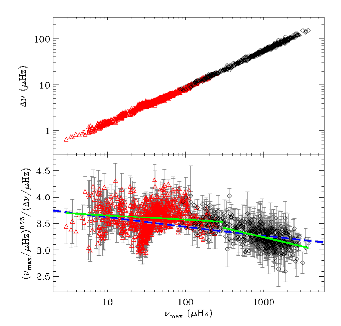
It has been well established for both main-sequence and red-giant stars that $\nu_{\rm max}$ and $\Delta\nu$ follow a power law relation (Stello et al., 2009a; Hekker et al., 2009; Mosser et al., 2010; Hekker et al., 2011b, a):

$$\Delta\nu=\alpha(\nu_{\rm max}/\mu\rm Hz)^{\beta}\>.$$ (3)

Figure 1 shows this relation for the entire Kepler sample in our analysis. Although the relation appears to be constant over several orders of magnitude, Mosser et al. (2010) and Huber et al. (2010) noted that the slope is different for red-giant and main-sequence stars. This can be illustrated more clearly by removing the luminosity dependence by raising $\nu_{\rm max}$ to the power of 0.75, yielding

$$\frac{(\mbox{$\nu_{\rm max}$}/\mbox{$\mu$Hz})^{0.75}}{\mbox{$\Delta\nu$}/\mbox{$\mu$Hz}}\propto\left(\frac{M}{M_{\sun}}\right)^{0.25}\left(\frac{T_{\rm eff}}{T_{\rm eff,\sun}}\right)^{-0.375}\>.$$ (4)

Table 1Coefficients of the $\Delta\nu$-$\nu_{\rm max}$ relation.

Method	$\alpha,\beta$	$\alpha,\beta$	# of stars
	$\mbox{$\nu_{\rm max}$}<300\mbox{$\mu$Hz}$	$\mbox{$\nu_{\rm max}$}>300\mbox{$\mu$Hz}$
A2Z	0.259(3),0.765(2)	0.25(1),0.779(7)	919,257
COR	0.267(3),0.761(2)	0.23(1),0.789(6)	1150,415
OCT	0.263(3),0.763(2)	0.20(1),0.811(7)	1082,281
SYD	0.267(2),0.760(2)	0.22(1),0.797(5)	1228,458

A2Z - Mathur et al. (2010a), COR - Mosser & Appourchaux (2009); Mosser et al. (2011b), OCT - Hekker et al. (2010b), SYD - Huber et al. (2009).

The lower panel of Figure 1 displays this ratio as function of $\nu_{\rm max}$. The distribution shows a prominent diagonal structure around $\mbox{$\nu_{\rm max}$}\sim 20-50\mbox{$\mu$Hz}$, which we identify as the red clump, comprising He-core burning red giant stars (see Bedding et al., 2011; Mosser et al., 2011a, c). It is evident that the power law becomes steeper as $\nu_{\rm max}$ increases. To measure this effect, we fitted Equation (3) to the sample in two groups subdivided at $\mbox{$\nu_{\rm max}$}=300\mbox{$\mu$Hz}$, which roughly marks the transition from low-luminosity red giants to subgiants. The best-fitting power laws for the SYD pipeline are shown as solid green lines in the lower panel of Figure 1, and the results for each pipeline with values for both long- and short cadence data are listed in Table 1. The difference in the coefficients between red giant and main-sequence stars is significant, and should be noted when using the relation for determining $\Delta\nu$ from $\nu_{\rm max}$. For $\nu_{\rm max}$ close to the solar value, for example, the use of a power-law relation calibrated to red-giant stars would lead to an underestimation in $\Delta\nu$ by $\sim$ 10%. For comparison, the blue dashed line in the lower panel of Figure 1 shows the relation derived by Stello et al. (2009a) using a sample including both main-sequence and red-giant stars.

How do our observed values of $\nu_{\rm max}$ and $\Delta\nu$ compare with evolutionary models? The upper panel of Figure 2 compares the observed distributions with solar-metallicity models with masses 1.0$M_{\sun}$, 1.3$M_{\sun}$ and 2.0$M_{\sun}$ (solid lines), which roughly correspond to the lower bound, median and upper bound of the mass distribution derived by Kallinger et al. (2010a) and Chaplin et al. (2011a). The model values for $\nu_{\rm max}$ and $\Delta\nu$ have been calculated using Equations (1) and (2). Additionally, we have color-coded the mass of each star calculated using Equations (1) and (2) with the observed values of $\nu_{\rm max}$ and $\Delta\nu$  adopting the effective temperature listed in the Kepler Input Catalog (KIC, Brown et al., 2011). The observed and theoretical masses in this plot essentially correspond to a comparison of the so-called direct method and grid-based method of estimating asteroseismic masses (see, e.g., Gai et al., 2011), assuming solar metallicity.

Figure 2.— Upper panel: Observed values of $\nu_{\rm max}^{0.75}$/$\Delta\nu$ versus $\nu_{\rm max}$ (symbols) compared to solar-metallicity ($Y=0.273$, $Z=0.0198$) models with 1$M_{\sun}$, 1.3$M_{\sun}$ and 2.0$M_{\sun}$ (solid lines). Asteroseismic masses are color-coded as indicated in the plot. Typical error bars for different ranges of $\nu_{\rm max}$ are indicated near the bottom of the plot. Lower panel: Same as top panel but with the effective temperature dependence removed (see Equation (4)) and omitting model tracks. Symbol types and colors are the same as in Figure 1. The green solid lines show linear fits to the linear-log plot for the same intervals of $\nu_{\rm max}$ as in Figure 1.

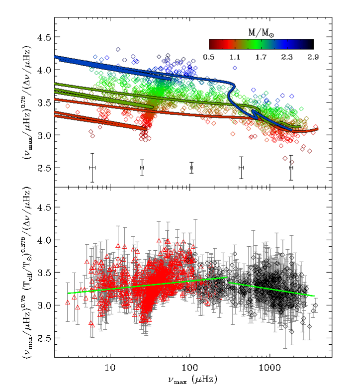
As noted by Kallinger et al. (2010b) and Huber et al. (2010), the spread in stellar mass is pronounced on the red giant branch, while for less-evolved stars the spread in observations is weaker and the models almost overlap. The overall agreement between the models and the data is very good, and we do not observe any significant offset of the models with respect to the observations. It is also remarkable how well the models of different masses track the He-core-burning red clump. Although the spread of data points about the models for main-sequence stars can be explained by measurement uncertainties, we note that stellar population models presented by Silva Aguirre et al. (2011) yield evidence that the Kepler sample is on average metal-poor, which can have a some impact on the $\Delta\nu$-$\nu_{\rm max}$ relation of main-sequence stars (see Huber et al., 2010). As noted by Silva Aguirre et al. (2011), however, the measurement uncertainties are currently too large to test a metallicity influence on the scaling relations.

What causes the different $\Delta\nu$-$\nu_{\rm max}$ power-law relations for evolved and unevolved stars? The scaling relation in Equation (4) suggests that the change in slope for the unevolved stars must be partially due to a variation in effective temperature. To test this hypothesis, we again used the effective temperatures listed in the Kepler Input Catalog to model this dependency using Equation (4). The result is shown in the lower panel of Figure 2. As expected, correcting for the higher average effective temperatures of main-sequence stars compared to red giants removes the gradient in the distribution. Subdividing the sample again at $\mbox{$\nu_{\rm max}$}=300\mbox{$\mu$Hz}$, we find a positive slope for the red giant sample and a negative slope for main-sequence stars (solid green lines). These variations are qualitatively in agreement with different mass distributions in the sample: while for red giants $\nu_{\rm max}$ is correlated to stellar mass for He-core burning stars (Mosser et al., 2011a, c), main-sequence stars with higher $\nu_{\rm max}$ are generally low-mass stars (see, e.g., Chaplin et al., 2011a). Without mass estimates independent of asteroseismic scaling relations, however, it is not possible to make further quantitative conclusions about the distribution.

4. Amplitudes

4.1. The L/M Scaling Relation

KB95 suggested that model predictions by Christensen-Dalsgaard & Frandsen (1983) implied a scaling for velocity amplitudes of

$$A_{\rm vel}\propto\left(\frac{L}{M}\right)^{s}\>,$$ (5)

with $s=1$. They further argued that the oscillation amplitude $A_{\lambda}$ observed in photometry at a wavelength $\lambda$ is related to the velocity amplitude:

$$A_{\lambda}\propto\frac{v_{\rm osc}}{\lambda T_{\rm eff}^{r}}\>.$$ (6)

The exponent $s$ has since been revised in the range of roughly $s=0.7-1.3$ both theoretically (Houdek et al., 1999a; Houdek, 2006; Samadi et al., 2007), as well as observationally using red-giant stars (Gilliland, 2008; Dziembowski & Soszyński, 2010; Mosser et al., 2010; Stello et al., 2010), main-sequence stars (Verner et al., 2011a) and an ensemble of main-sequence and red-giant stars (Baudin et al., 2011). The value for $r$ has so far been chosen to be either $r=1.5$ (assuming adiabatic oscillations) or $r=2.0$ (the best-fitting coefficient found by KB95 for classical pulsators).

Since our sample spans a large range in effective temperature, we must account for the spectral response of the Kepler bandpass to compare predictions made with Equation (6) to our observations. To do so, we used the expression for the bolometric amplitude given by KB95 and converted these values to amplitudes observed in the Kepler bandpass, as follows:

$$A_{\rm Kp}\propto\left(\frac{L}{M}\right)^{s}\frac{1}{T_{\rm eff}^{r-1}c_{\rm K}(T_{\rm eff})}\>,$$ (7)

with $c_{\rm K}$ being the bolometric correction factor as a function of effective temperature, given by Ballot et al. (2011):

$$c_{\rm K}(T_{\rm eff})=\left(\frac{T_{\rm eff}}{5934\rm K}\right)^{0.8}\>.$$ (8)

The reason for choosing to correct the model amplitudes rather than the observed values is that effective temperatures for most of the stars in our sample are rather uncertain, and we hence prefer not to perform the correction on the observed amplitudes.

Figure 3.— (a) Oscillation amplitude versus $\nu_{\rm max}$ for the entire Kepler sample. Symbol types and colors are the same as in Figure 1. The position of the Sun is also marked. (b) Same as panel (a) but with asteroseismic masses color-coded. Error bars have been omitted for clarity. Solid lines show the 1.0, 1.3 and 2.0 $M_{\sun}$ solar-metallicity ($Y=0.273$, $Z=0.0198$) models scaled using Equation (7) with typical values of $r=2$ and $s=0.8$. (c) Same as panel (b) but using Equation (9) with coefficients determined by fitting the model tracks to observations. (d) Same as panel (c) but with best fitting coefficients determined by comparing observed amplitudes with calculated amplitudes using asteroseismic masses and radii (see text for details).

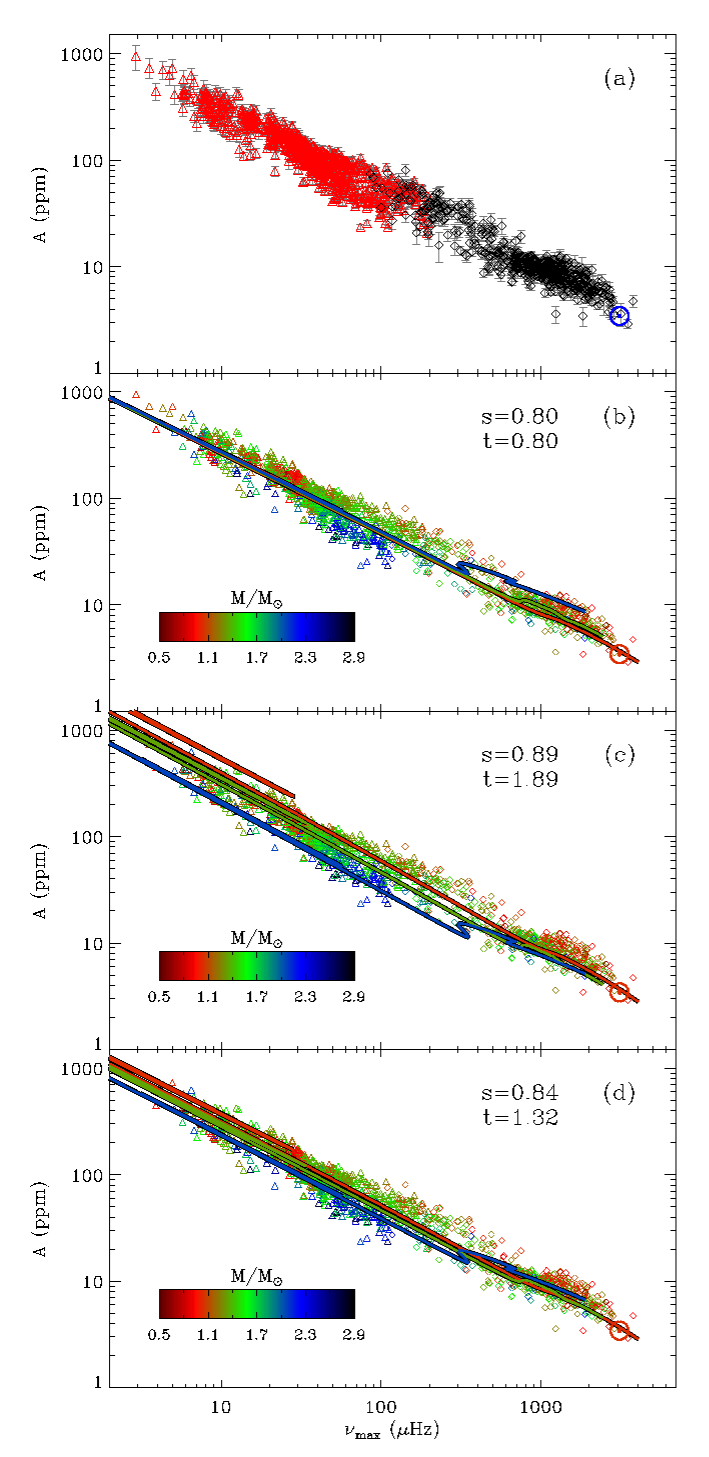
Figure 3(a) shows the observed amplitudes for the full Kepler sample as a function of $\nu_{\rm max}$. The spread is much larger than the typical measurement uncertainties. As first noted by Huber et al. (2010) and later confirmed by Mosser et al. (2011a), Mosser et al. (2011c) and Stello et al. (2011), this spread in the amplitude-$\nu_{\rm max}$ relation for red giants is related to a spread in mass. To demonstrate this, Figure 3(b) shows the same plot but color-coded by stellar masses, as calculated in the previous section. We observe that, particularly for low-luminosity red giants, the higher-mass stars show lower amplitudes than lower-mass stars for a given $\nu_{\rm max}$. For unevolved stars we can tentatively identify the same trend, although the separation is less clear.

The observation of a mass dependence for a given $\nu_{\rm max}$ indicates that Equation (7) should be revised to include an additional mass dependence. To demonstrate this, solid lines in Figure 3(b) show model tracks with different masses scaled using typical values of $r=2$ and $s=0.8$ in Equation (7). The $(L/M)^{s}$ scaling clearly fails to reproduce the observed spread on the red-giant branch, but predicts a strong mass dependence for unevolved stars, contrary to what is observed.

An obvious way to account for an additional mass dependence is to rearrange Equation (7) as follows:

$$A_{\rm Kp}\propto\frac{L^{s}}{M^{t}T_{\rm eff}^{r-1}c_{\rm K}(T_{\rm eff})}\>.$$ (9)

Note that such a formulation has been introduced by Kjeldsen & Bedding (2011) (hereafter KB11) and has also been used by Stello et al. (2011) in the Kepler study of cluster red giants. To evaluate the coefficients that best reproduce our observations, we again used models with masses 1.0$M_{\sun}$, 1.3$M_{\sun}$ and 2.0$M_{\sun}$ and calculated their expected amplitudes according to Equation (9) for a given set of $s$, $t$ and $r$. The agreement of models and observations was evaluated as follows: For each observed amplitude, we interpolated each model track to obtain the model amplitude at the observed $\nu_{\rm max}$ value. We then calculated the minimum squared deviation of the observed amplitude to the three model amplitudes, normalized by the measurement uncertainty. The parameters $s$, $t$ and $r$ were then optimized using a least-squares fit. Note that for simplicity we have only used model values below the tip of the red-giant branch, since an inclusion of later evolutionary stages would require the identification of all red-clump stars in our sample which is beyond the scope of this paper.

First tests quickly showed that the strong correlation between effective temperature and luminosity made an independent determination of $s$, $t$ and $r$ impossible. Following Stello et al. (2011), we have therefore fixed the value to $r=2$. The best-fitting parameters are $s=0.886\pm 0.002$ and $t=1.89\pm 0.01$, with uncertainties estimated by repeating the fitting procedure 1000 times using amplitudes drawn from a random distribution with a scatter corresponding to the $1\,\sigma$ measurement uncertainties (scaled so that reduced $\chi^{2}=1$ for the original data). The parameter uncertainties were then estimated by calculating the standard deviation of the resulting distribution for each coefficient.

The scaled model tracks in Figure 3(c) using these coefficients reproduce a mass spread in amplitude for red giants, with higher-mass stars showing lower amplitudes for a given $\nu_{\rm max}$, as observed by Huber et al. (2010), Mosser et al. (2011a), Stello et al. (2011) and Mosser et al. (2011c). For unevolved stars, the model amplitudes now show less dispersion but appear to systematically underestimate amplitudes for both subgiant and main-sequence stars.

Figure 4.— Observed versus calculated amplitudes for the best-fitting coefficients in Equation (9), using radii and masses determined using the scaling relations for $\nu_{\rm max}$ and $\Delta\nu$. The dashed blue line shows the 1:1 relation. The position of the Sun is also shown.

The method presented above assumes that the excess spread of amplitudes at a given $\nu_{\rm max}$ is entirely due to a spread in stellar mass. A more sophisticated approach is to account for the actual mass distribution by directly using masses and radii of the sample estimated using $\nu_{\rm max}$ and $\Delta\nu$ in Equations (1) and (2). We again used the effective temperatures from KIC and evaluated Equation (9) for each value of $s$ and $t$ directly using these asteroseismic masses and radii. The corresponding best-fitting parameters in this case were $s=0.838\pm 0.002$ and $t=1.32\pm 0.02$, and the scaled model tracks with these parameters are shown in Figure 3(d). The spread of the model tracks on the red giant branch is now considerably reduced, better matching the observations, and the overall fit for less evolved stars is also improved.

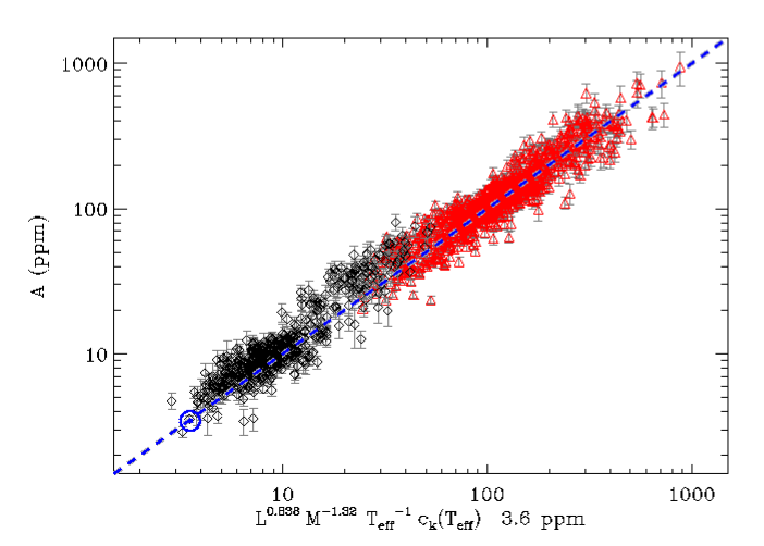
Figure 4 compares the observed and calculated amplitudes using $s=0.838$ and $t=1.32$, showing good agreement along the 1:1 line over the entire range of $\nu_{\rm max}$. The residuals between observed and calculated amplitudes over the full range of $\nu_{\rm max}$ show a standard deviation of about 25%, which is consistent with the typical uncertainties in the adopted stellar properties (estimated from propagating the uncertainties in $\nu_{\rm max}$ and $\Delta\nu$ and assuming an uncertainty of 200 K in $T_{\rm eff}$) and the measurement uncertainties in the observed amplitudes. We do see an overall bias of about 9%, with calculated amplitudes being systematically underestimated when scaling from the solar value. This bias is stronger for unevolved stars with $\mbox{$\nu_{\rm max}$}>300\mbox{$\mu$Hz}$ (15%) than for evolved stars $\mbox{$\nu_{\rm max}$}<300\mbox{$\mu$Hz}$ (7%). An explanation for this bias might be additional physical differences between the Sun and our Kepler sample, which influence oscillation amplitudes but have not yet been taken into account.

Our best-fitting values for $s$ and $t$ using asteroseismic masses and radii are significantly different to Stello et al. (2011), who found $s=0.90\pm 0.02$ and $t=1.7\pm 0.1$ using independently determined properties of cluster red giants in the Kepler field. This difference is presumably due to the fact that our sample includes a much wider range of evolutionary states. Indeed, repeating our analysis using only red giants in a $\nu_{\rm max}$ range similar to that used by Stello et al. (2011) yields coefficients which are in better agreement. Remaining differences could potentially be due to metallicity effects which have been suggested to have a significant influence on oscillation amplitudes (Samadi et al., 2010) or systematic errors when estimating stellar properties through the direct method of using $\nu_{\rm max}$ and $\Delta\nu$. Nevertheless, all methods confirm that scaling relations with a separate mass and luminosity dependence better reproduce the observed amplitudes from the main sequence to red giants.

4.2. The KB11 Scaling Relation

Kjeldsen & Bedding (2011) recently argued that amplitudes of solar-like oscillations should scale in proportion to fluctuations due to granulation. They proposed a revised scaling relation for velocity amplitudes:

$$A_{\rm vel}\propto\frac{L\tau_{\rm osc}^{0.5}}{M^{1.5}T_{\rm eff}^{2.25}}\>,$$ (10)

where $\tau_{\rm osc}$ is the mode lifetime.

Using the same arguments as in the previous section, the KB11 relation predicts photometric amplitudes in the Kepler bandpass as follows:

$$A_{\rm Kp}\propto\frac{L\tau_{\rm osc}^{0.5}}{M^{1.5}T_{\rm eff}^{1.25+r}c_{\rm k}(T_{\rm eff})}\>.$$ (11)

They also suggested the following relation for the granulation power in intensity measured at $\nu_{\rm max}$:

$$P_{\rm int}(\nu_{\rm max})\propto\frac{L^{2}}{M^{3}T_{\rm eff}^{5.5}}\>.$$ (12)

First results on granulation properties of Kepler red-giant stars by Mathur et al. (2011) have shown promising agreement. More recently, Mosser et al. (2011c) confirmed the proportionality between mode amplitudes and the granulation power at $\nu_{\rm max}$ for a large sample of red giants, but found that the absolute values calculated using Equations (11) and (12) were offset from the observed values. Here we extend this comparison to include also main-sequence stars.

To test the relation, we used the solar granulation power at $\nu_{\rm max}$ determined by our analysis of VIRGO data, which yielded a mean value of $P_{\rm int,\sun}=0.19\pm 0.02$ ppm${}^{2}\mu$Hz^-1. The upper panel of Figure 5 compares the proposed relation in Equation (12), again using asteroseismic masses and radii, as well as effective temperatures from KIC. We observe that the calculated values are systematically too high for main-sequence stars, and systematically too low for red giants, the latter being in agreement with the results by Mosser et al. (2011c).

Figure 5.— Upper panel: Observed versus calculated granulation power at $\nu_{\rm max}$ using Equation (12). Lower panel: Observed versus calculated amplitudes using Equation (11) and assuming a solar mode lifetime for all stars. The dashed blue line shows the 1:1 relation in both panels, and the position of the Sun is marked.

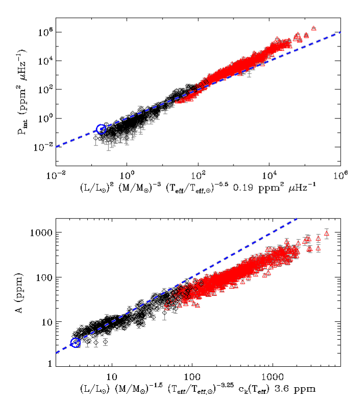
In order to compare observed with calculated amplitudes using Equation (11), estimates of the mode lifetimes are required. While it is well established that mode lifetimes in giants are significantly longer than in main-sequence stars (De Ridder et al., 2009; Chaplin et al., 2009; Hekker et al., 2010a; Huber et al., 2010; Baudin et al., 2011), $\tau_{\rm osc}$ is not very well constrained for stars spanning such a large range in evolution as considered in our sample. We have therefore decided to neglect the influence of $\tau_{\rm osc}$ in Equation (11) in our study. The lower panel of Figure 5 shows the comparison between observed and calculated amplitudes using Equation (11) and assuming solar mode lifetime for all stars. We observe that the revised scaling relation works well for main-sequence and subgiant stars, but predicts amplitudes that are systematically too high for red giants, again in agreement with Mosser et al. (2011c).

We note that the upper panel of Figure 5 displays an apparent systematic difference in the granulation power at $\nu_{\rm max}$ in the overlapping region of the long-cadence and short-cadence sample. This effect is due to a systematic difference of the modelled background noise level for stars oscillating close to the long-cadence Nyquist frequency (283$\mu$Hz). We have confirmed that this has a negligible effect on the measured amplitudes, as is evident by the consistent overlap of datapoints in the bottom panel of Figure 5.

As noted by Kjeldsen & Bedding (2011), the observed differences are not unexpected since the relation does not take into account potential differences in the intensity contrast between dark and bright regions on the stellar surface. While our study confirms the relation between mode amplitudes and granulation power for stars ranging from the main-sequence to the red-giant branch, it demonstrates that the link between velocity and intensity measurements is not yet fully understood for amplitude scaling relations.

4.3. Stellar Activity & Amplitudes

The offset between observed and calculated amplitudes for main-sequence stars noted in Section 4.1 suggests that there might be an additional physical dependency which is not yet taken into account. Increased stellar activity and magnetic fields are known to decrease pulsation amplitudes in the Sun (Chaplin et al., 2000; Komm et al., 2000), and have been suggested as a possible cause for the unexpected low amplitudes of oscillations in active stars (Mosser et al., 2009; Dall et al., 2010). The first direct evidence for an influence of stellar activity on oscillation amplitudes for a star other than the Sun has been found in the F-star HD 49933 (García et al., 2010). As discussed by KB11, these amplitude changes may be due to changes in the mode lifetimes.

Recently, Chaplin et al. (2011b) reported the discovery for main-sequence and subgiant stars observed with Kepler that oscillations are less likely to be detected in stars with higher activity. This led them to conclude that, just like for the Sun, increased stellar activity suppresses mode amplitudes. Kepler results have furthermore shown that the detection rate seems to be considerably lower for subgiant stars with $\mbox{$\nu_{\rm max}$}\sim 400-900\,\mbox{$\mu$Hz}$ (Chaplin et al., 2011a, c; Silva Aguirre et al., 2011). This was tentatively explained by increased magnetic activity in this stage of stellar evolution, as predicted by Gilliland (1985). While it is known that some detection bias due to instrumental artefacts might be present in the frequency range from 200-500 $\mu$Hz (García et al., 2011), both discoveries strongly suggest that activity must be considered when calculating amplitudes.

While Chaplin et al. (2011b) used a simple detection criterion, we attempt here to confirm and quantify their discovery by correlating measured pulsation amplitudes with stellar activity. Several studies have been devoted to stellar activity and variability in the Kepler field (Basri et al., 2010; Debosscher et al., 2011; Ciardi et al., 2011) with various definitions of activity measures. Since our study covers a large range of oscillation timescales and amplitudes, we need to define an activity measure which separates variability due to oscillations from variations due to activity, and at the same time remains sensitive to local minima and maxima in the light curve. To do this, we first smoothed each light-curve with a quadratic Savitzky-Golay filter (Savitzky & Golay, 1964) with a full-width corresponding to 20 times the determined oscillation period, and then measured the absolute maximum deviation of the smoothed curve from its mean. We denote this measure of activity as $r_{\rm sg}$. Note that we have repeated the analysis with smoothing widths ranging between 10-50 times the oscillation period, but found not significant difference in the results. When evaluating $r_{\rm sg}$, it must be kept in mind that our sample includes light curves with two very different timebases ($\sim$ 30 d for short cadence, and $\sim$500 d for long cadence). The samples therefore probe different activity time scales, and have hence been separated in the subsequent analysis.

Figure 6.— Amplitude versus $\nu_{\rm max}$ showing only stars observed in short cadence, with the logarithm of the activity range color coded. Red and blue points correspond to high and low activity, respectively. The position of the Sun with a color corresponding to the mean solar activity is also shown.

To correct our activity measure for the influence of shot noise, we performed the following simulations. For each target light curve, we produced synthetic timeseries including a sinusoidal variation with an amplitude corresponding to the measured $r_{\rm sg}$ value. We then added white noise with a standard deviation corresponding to the apparent magnitude of the target, which was estimated from the minimal noise levels given in Gilliland et al. (2010a) and Jenkins et al. (2010). We then measured $r_{\rm sg}$ for the synthetic light curve as described above, and calculated the difference between this value and the value of $r_{\rm sg}$ measured from the noise-free time series. This process was repeated 500 times for each star, and the median of the resulting distribution was taken as the correction value for the observed $r_{\rm sg}$. In summary, it was found that the typical correction values were about 8% for short-cadence data, and $<1\%$ for long-cadence data.

Figure 7.— Upper panel: Residuals of observed amplitude divided by the calculated amplitudes using Equation 9 versus the logarithm of the activity measure for all stars with $\mbox{$\nu_{\rm max}$}>1000\mbox{$\mu$Hz}$. The red solid line shows an unweighted linear fit. Middle panel: Same as the upper panel but for all stars with $\mbox{$\nu_{\rm max}$}=300-1000\,\mbox{$\mu$Hz}$. Lower panel: Same as upper panel but for all long-cadence stars ($\mbox{$\nu_{\rm max}$}<300\mbox{$\mu$Hz}$).

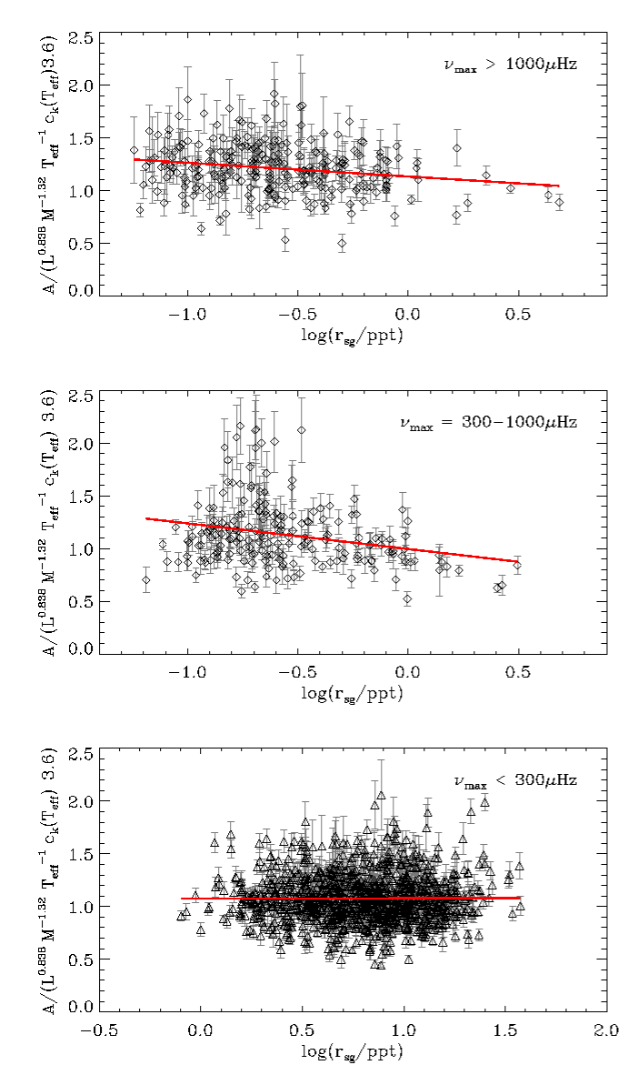
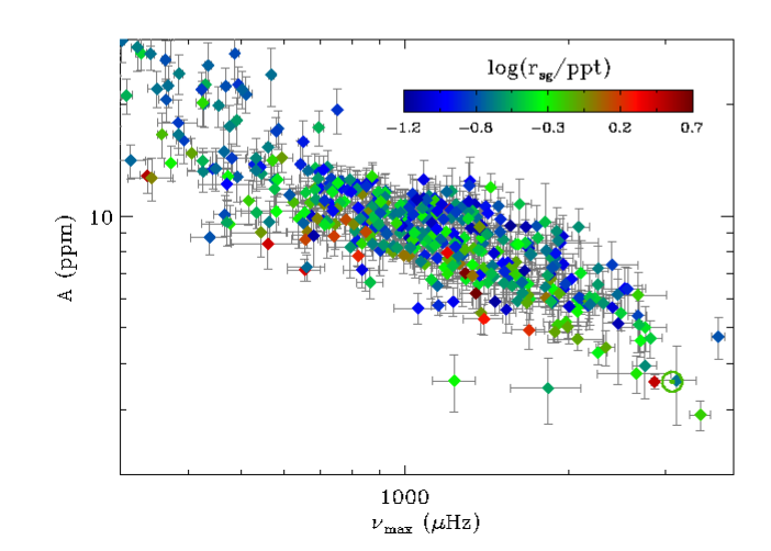
Figure 6 shows the amplitude-$\nu_{\rm max}$ relation for the short cadence sample, with the logarithm of the activity measure color-coded. We see that the most active stars (shown in red) have generally lower amplitudes than less active stars (shown in blue). As found by Chaplin et al. (2011b), the Kepler sample is generally less active than the average Sun ($r_{\rm sg,\sun}=0.7$ ppt), in agreement with the bias towards lower predicted amplitudes found in the previous section. To quantify this, we first removed the dependence of oscillation amplitudes on stellar properties by dividing them by the calculated amplitudes using Equation (9) with the best-fitting coefficients derived in the previous section. The resulting normalized amplitudes are plotted versus the logarithm of the activity measure in Figure 7.

Figure 7 is split into three ranges of $\nu_{\rm max}$, roughly dividing stars on the main-sequence (top panel), subgiants (middle panel) and red giants (bottom panel). The influence of activity on amplitudes appears the strongest for subgiant stars, followed by a weak correlation for main-sequence stars and no visible correlation for red giants. Unweighted linear fits to the linear-log plots yield slopes of $-0.13\pm 0.04$, $-0.24\pm 0.07$ and $0.00\pm 0.02$, respectively. While the correlations for unevolved stars are formally significant, a thorough comparison with other methods has shown that the correlation for subgiant stars is only confirmed in three out of six methods, while the results for main-sequence and red-giant stars are consistent with zero within 3$\sigma$ for all methods. Although this comparison cautions us not to draw any definite conclusions, we note that the exponential decrease of amplitude with increasing stellar activity for subgiants would be in-line with both observational and theoretical evidence for enhanced magnetic activity in these stars (Gilliland, 1985; Chaplin et al., 2011a). A confirmation of the results presented here will have to await longer timeseries (in particular for short cadence data) which will allow a better estimate of the activity measure and reduce the uncertainty in the adopted stellar properties through better constraints on $\nu_{\rm max}$ and $\Delta\nu$. This will then allow a more in-depth investigation of additional physical influences on oscillation amplitudes such as stellar activity and metallicity (Samadi et al., 2010).

5. The Cool Edge of the Instability Strip

The cool edge of the instability strip is widely believed to be the dividing line between coherent pulsations driven by the opacity ($\kappa$) mechanism and solar-like oscillations driven by convection. Considerable work has been devoted to establishing this boundary both empirically using $\delta$ Scuti and $\gamma$ Doradus stars (see, e.g., Breger, 1979; Pamyatnykh, 2000) as well as theoretically (see, e.g., Houdek et al., 1999b; Houdek, 2000; Xiong & Deng, 2001; Dupret et al., 2004, 2005). The large number of stars for which Kepler has detected oscillations now allows the first test of this boundary from “the cool side”, using solar-like oscillations.

Figure 8.— $\nu_{\rm max}$ versus effective temperature for all stars in our sample. Color codes refer to the logarithm of the pulsation amplitude, with blue and red colors marking the highest and lowest amplitudes, respectively. The dashed line shows the empirically determined cool edge of the instability strip from observations of $\delta$ Scuti stars. The theoretical cool edge for the fundamental radial mode of $\delta$ Scuti pulsations is shown for a 1.7 $M_{\sun}$ model by Houdek (2000) (solid circle) and a range of masses by Dupret et al. (2005) (dashed-dotted line). Black solid lines are solar-metallicity BaSTI evolutionary tracks with masses as indicated in the plot. The star symbol indicates the first detection of hybrid solar-like and $\delta$ Scuti oscillations by Antoci et al. (2011).

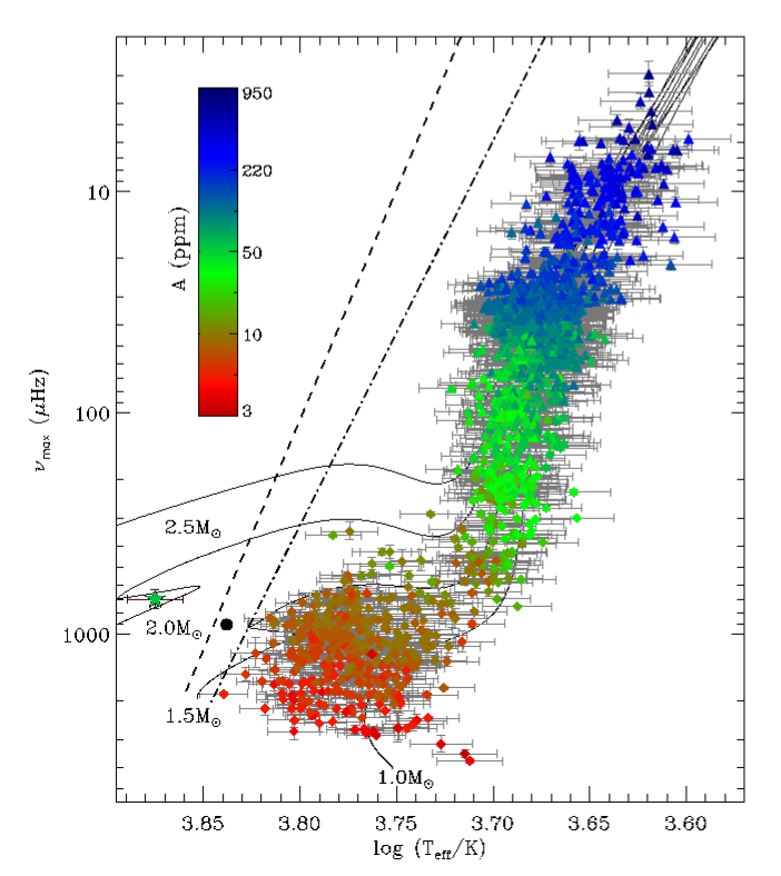
Figure 8 shows all stars of our sample in a modified H-R diagram, in which we have replaced luminosity with $1/\mbox{$\nu_{\rm max}$}$. We also show the empirically determined cool edge of the instability strip taken from Pamyatnykh (2000) as a dashed line, as well as the theoretical cool edge for the fundamental radial mode of $\delta$ Scuti pulsations for a 1.7$M_{\sun}$ model taken from Houdek (2000) (filled circle) and for a range of masses by Dupret et al. (2005) (dashed-dotted line). To convert the lines from the $\log L-\log T_{\rm eff}$ to the $\log\mbox{$\nu_{\rm max}$}-\log T_{\rm eff}$ plane, we determined the closest matching grid point of evolutionary tracks with different masses to the $\log L-\log T_{\rm eff}$ relation, and then fitted a straight line to the resulting points in the $\log\mbox{$\nu_{\rm max}$}-\log T_{\rm eff}$ plane. This has been done both for BaSTI and a set of ASTEC (Christensen-Dalsgaard, 2008) evolutionary models, and both sets of models yielded consistent results. The empirically determined cool edges taken from Pamyatnykh (2000) in Figure 8 are:

$$\log(T_{\rm eff}/K)=-0.045\log(L/L_{\sun})+3.893$$ (13)

$$\log(T_{\rm eff}/K)=0.048\log(\mbox{$\nu_{\rm max}$}/\mbox{$\mu$Hz})+3.702\>.$$ (14)

Equation (14) appears in good agreement with the hottest stars for which solar-like oscillations are observed. However, it is important to note that the recent work by Pinsonneault et al. (2011) and Molenda-Żakowicz et al. (2011) suggest that many stars are significantly hotter than the effective temperatures given in KIC, with differences of up to 250 K. With this in mind, the fact that we observe stars close to the theoretical limit is evidence that the separation between the classical and stochastic pulsations is probably not a sharp dividing boundary. Indeed, we indeed do not observe a gradual decrease in amplitude towards the cool edge of the instability strip and the recent discovery of solar-like and $\delta$ Scuti oscillations in HD 187547 by Antoci et al. (2011) using Kepler data has confirmed the existence of hybrid pulsators (see star symbol in Figure 8). Interestingly, the observed amplitude for this star is roughly a factor four higher than expected from the traditional scaling relations discussed in this paper. This was tentatively explained by the increased mode lifetimes which are roughly 4-5 times higher than expected from scaling relations based on effective temperature (Chaplin et al., 2009; Baudin et al., 2011).

Figure 9.— H-R diagram of the low-luminosity region shown in Figure 8, comparing stars for which no oscillations have been detected (open black diamonds) with our sample of detections (red filled diamonds). A typical error bar for both samples is shown in the top region of the plot. The dashed line, dashed-dotted line and filled circle are the same as in Figure 8. The star symbol indicates the first detection of hybrid solar-like and $\delta$ Scuti oscillations by Antoci et al. (2011).

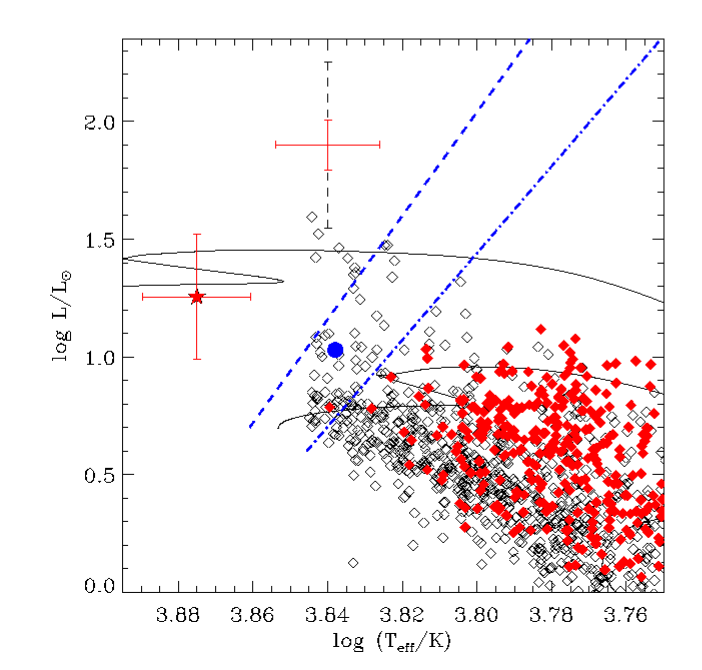
To test the cool edge of the instability strip more quantitatively, we must account for selection effects. Figure 9 shows a close-up of the main-sequence region of the HRD, this time plotting luminosity on the ordinate and including stars for which we did not find evidence for oscillations. Luminosities for stars without detections have been calculated based on values in the KIC assuming an uncertainty on the radius of 40% (Verner et al., 2011b), while for stars with detections Equations (1) and (2) were used. Although the error bars are large, we observe an excess of hot stars for which no oscillations have been detected, indicating that the observed cut-off in detections may not entirely due be due to selection bias. We therefore conclude that the empirical red-edge given in Equations (13) and (14) gives a good approximation for the transition between opacity driven and solar-like oscillations. Further work will be needed to quantify this observation and compare the results with theoretical models of excitation and damping of solar-like oscillations, as well as possible further detections of hybrid solar-like oscillations and classical pulsation in hot stars.

6. Conclusions

We have studied global oscillation properties in $\sim$1700 stars observed by Kepler to test asteroseismic scaling relations. Our main findings can be summarized as follows:

• By comparing evolutionary models with observations, we have shown that the scaling relations for $\nu_{\rm max}$ and $\Delta\nu$ are in qualitative agreement with observations for evolutionary stages spanning from the main-sequence to the He-core burning phase of red giants. The difference in the $\Delta\nu$-$\nu_{\rm max}$ relation between evolved and unevolved stars can be explained by different distributions of effective temperature and stellar mass, in agreement with what is expected from the scaling relations. A more quantitative test of scaling relations for $\nu_{\rm max}$ and $\Delta\nu$ will have to await the determination of fundamental properties from independent methods such as spectroscopy and long-baseline interferometry.

• We have shown that $(L/M)^{s}$ scaling for oscillation amplitudes fails to reproduce the amplitude-$\nu_{\rm max}$ relation for red giants. We have verified that a revised scaling relation using a separate mass and luminosity dependence reproduces the observations better, and a relation with $L^{s}$ and $M^{t}$ coefficients of $s=0.838\pm 0.002$ and $t=1.32\pm 0.02$ matches amplitudes for field stars ranging from the main-sequence to the red clump to a precision of 25% when adopting stellar properties derived from scaling relations. The calculated amplitudes for main-sequence and subgiant stars in our sample are systematically underestimated by up to 15%, indicating that there might be an additional physical dependence which is not yet taken into account.

• We have investigated the connection of stellar activity with the suppression of oscillation amplitudes in main-sequence, subgiant and red-giant stars. We find evidence that the effect is strongest for subgiant stars, but caution that these results will have to await confirmation with longer time series providing a better estimate of the activity measure and reduced uncertainties on stellar properties used to calculated amplitudes. The present data do not yield strong evidence that stellar activity contributes significantly to the underestimation of calculated amplitudes for main-sequence stars.

• We have investigated the cool edge of the instability strip using detections of solar-like oscillations. We find good agreement with the empirically and theoretically determined cool edge using $\delta$ Scuti stars, but note that many stars showing solar-like oscillations may overlap with cooler $\delta$ Scuti stars, in agreement with the recent first discovery of hybrid solar-like and $\delta$ Scuti oscillations by Antoci et al. (2011).

References

- Aerts et al. (2010) Aerts, C., Christensen-Dalsgaard, J., & Kurtz, D. W. 2010, Asteroseismology
- Antoci et al. (2011) Antoci, V., et al. 2011, Nature, in press
- Ballot et al. (2011) Ballot, J., Barban, C., & van’t Veer-Menneret, C. 2011, A&A, 531, A124
- Basri et al. (2010) Basri, G., et al. 2010, ApJ, 713, L155
- Baudin et al. (2011) Baudin, F., et al. 2011, A&A, 529, A84
- Bedding (2011) Bedding, T. R. 2011, arXiv:1107.1723
- Bedding & Kjeldsen (2003) Bedding, T. R., & Kjeldsen, H. 2003, PASA, 20, 203
- Bedding et al. (2010) Bedding, T. R., et al. 2010, ApJ, 713, 935
- Bedding et al. (2011) —. 2011, Nature, 471, 608
- Belkacem et al. (2011) Belkacem, K., Goupil, M. J., Dupret, M. A., Samadi, R., Baudin, F., Noels, A., & Mosser, B. 2011, A&A, 530, A142
- Bonanno et al. (2008) Bonanno, A., Benatti, S., Claudi, R., Desidera, S., Gratton, R., Leccia, S., & Paternò, L. 2008, ApJ, 676, 1248
- Breger (1979) Breger, M. 1979, PASP, 91, 5
- Brown & Gilliland (1994) Brown, T. M., & Gilliland, R. L. 1994, ARA&A, 32, 37
- Brown et al. (1991) Brown, T. M., Gilliland, R. L., Noyes, R. W., & Ramsey, L. W. 1991, ApJ, 368, 599
- Brown et al. (2011) Brown, T. M., Latham, D. W., Everett, M. E., & Esquerdo, G. A. 2011, AJ, 142, 112
- Campante et al. (2010) Campante, T. L., Karoff, C., Chaplin, W. J., Elsworth, Y. P., Handberg, R., & Hekker, S. 2010, MNRAS, 408, 542
- Casagrande et al. (2010) Casagrande, L., Ramírez, I., Meléndez, J., Bessell, M., & Asplund, M. 2010, A&A, 512, A54
- Chaplin et al. (2000) Chaplin, W. J., Elsworth, Y., Isaak, G. R., Miller, B. A., & New, R. 2000, MNRAS, 313, 32
- Chaplin et al. (2008) Chaplin, W. J., Houdek, G., Appourchaux, T., Elsworth, Y., New, R., & Toutain, T. 2008, A&A, 485, 813
- Chaplin et al. (2009) Chaplin, W. J., Houdek, G., Karoff, C., Elsworth, Y., & New, R. 2009, A&A, 500, L21
- Chaplin et al. (2011a) Chaplin, W. J., et al. 2011a, Science, 332, 213
- Chaplin et al. (2011b) —. 2011b, ApJ, 732, L5
- Chaplin et al. (2011c) —. 2011c, ApJ, 732, 54
- Christensen-Dalsgaard (2004) Christensen-Dalsgaard, J. 2004, Sol. Phys., 220, 137
- Christensen-Dalsgaard (2008) Christensen-Dalsgaard, J. 2008, Ap&SS, 316, 13
- Christensen-Dalsgaard & Frandsen (1983) Christensen-Dalsgaard, J., & Frandsen, S. 1983, Sol. Phys., 82, 469
- Ciardi et al. (2011) Ciardi, D. R., et al. 2011, AJ, 141, 108
- Dall et al. (2010) Dall, T. H., Bruntt, H., Stello, D., & Strassmeier, K. G. 2010, A&A, 514, A25
- De Ridder et al. (2009) De Ridder, J., et al. 2009, Nature, 459, 398
- Debosscher et al. (2011) Debosscher, J., Blomme, J., Aerts, C., & De Ridder, J. 2011, A&A, 529, A89
- Dupret et al. (2004) Dupret, M., Grigahcène, A., Garrido, R., Gabriel, M., & Scuflaire, R. 2004, A&A, 414, L17
- Dupret et al. (2005) Dupret, M.-A., Grigahcène, A., Garrido, R., Gabriel, M., & Scuflaire, R. 2005, A&A, 435, 927
- Dziembowski & Soszyński (2010) Dziembowski, W. A., & Soszyński, I. 2010, A&A, 524, A88
- Edmonds & Gilliland (1996) Edmonds, P. D., & Gilliland, R. L. 1996, ApJ, 464, L157
- Flower (1996) Flower, P. J. 1996, ApJ, 469, 355
- Fröhlich et al. (1997) Fröhlich, C., et al. 1997, Sol. Phys., 170, 1
- Fusi-Pecci & Renzini (1976) Fusi-Pecci, F., & Renzini, A. 1976, A&A, 46, 447
- Gai et al. (2011) Gai, N., Basu, S., Chaplin, W. J., & Elsworth, Y. 2011, ApJ, 730, 63
- García et al. (2010) García, R. A., Mathur, S., Salabert, D., Ballot, J., Régulo, C., Metcalfe, T. S., & Baglin, A. 2010, Science, 329, 1032
- García et al. (2011) García, R. A., et al. 2011, MNRAS, 414, L6
- Gilliland (1985) Gilliland, R. L. 1985, ApJ, 299, 286
- Gilliland (2008) —. 2008, AJ, 136, 566
- Gilliland et al. (2010a) Gilliland, R. L., et al. 2010a, ApJ, 713, L160
- Gilliland et al. (2010b) —. 2010b, PASP, 122, 131
- Grevesse & Noels (1993) Grevesse, N., & Noels, A. 1993, in Origin and Evolution of the Elements, ed. N. Prantzos, E. Vangioni-Flam, & M. Casse, 15–25
- Hekker et al. (2010a) Hekker, S., Barban, C., Baudin, F., De Ridder, J., Kallinger, T., Morel, T., Chaplin, W. J., & Elsworth, Y. 2010a, A&A, 520, A60
- Hekker et al. (2009) Hekker, S., et al. 2009, A&A, 506, 465
- Hekker et al. (2010b) —. 2010b, MNRAS, 402, 2049
- Hekker et al. (2011a) —. 2011a, A&A, 530, A100
- Hekker et al. (2011b) —. 2011b, MNRAS, 414, 2594
- Hekker et al. (2011c) —. 2011c, A&A, 525, A131
- Houdek (2000) Houdek, G. 2000, in Astronomical Society of the Pacific Conference Series, Vol. 210, Delta Scuti and Related Stars, ed. M. Breger & M. Montgomery, 454–+
- Houdek (2006) Houdek, G. 2006, in ESA Special Publication, Vol. 624, Proceedings of SOHO 18/GONG 2006/HELAS I, Beyond the spherical Sun
- Houdek et al. (1999a) Houdek, G., Balmforth, N. J., Christensen-Dalsgaard, J., & Gough, D. O. 1999a, A&A, 351, 582
- Houdek et al. (1999b) Houdek, G., Balmforth, N. J., Christensen-Dalsgaard, J., & Gough, D. O. 1999b, in Astronomical Society of the Pacific Conference Series, Vol. 173, Stellar Structure: Theory and Test of Connective Energy Transport, ed. A. Gimenez, E. F. Guinan, & B. Montesinos, 317
- Huber et al. (2009) Huber, D., Stello, D., Bedding, T. R., Chaplin, W. J., Arentoft, T., Quirion, P., & Kjeldsen, H. 2009, Communications in Asteroseismology, 160, 74
- Huber et al. (2010) Huber, D., et al. 2010, ApJ, 723, 1607
- Huber et al. (2011) —. 2011, ApJ, 731, 94
- Jenkins et al. (2010) Jenkins, J. M., et al. 2010, ApJ, 713, L120
- Kallinger et al. (2010a) Kallinger, T., et al. 2010a, A&A, 522, A1
- Kallinger et al. (2010b) —. 2010b, A&A, 509, A77
- Karoff et al. (2010) Karoff, C., Campante, T. L., & Chaplin, W. J. 2010, arXiv:1003.4167
- Kjeldsen & Bedding (1995) Kjeldsen, H., & Bedding, T. R. 1995, A&A, 293, 87
- Kjeldsen & Bedding (2011) —. 2011, A&A, 529, L8
- Kjeldsen et al. (2008) Kjeldsen, H., et al. 2008, ApJ, 682, 1370
- Komm et al. (2000) Komm, R. W., Howe, R., & Hill, F. 2000, ApJ, 531, 1094
- Leavitt (1908) Leavitt, H. S. 1908, Annals of Harvard College Observatory, 60, 87
- Mathur et al. (2010a) Mathur, S., et al. 2010a, A&A, 511, A46
- Mathur et al. (2010b) —. 2010b, A&A, 518, A53
- Mathur et al. (2011) —. 2011, ApJ, in press
- Michel et al. (2009) Michel, E., Samadi, R., Baudin, F., Barban, C., Appourchaux, T., & Auvergne, M. 2009, A&A, 495, 979
- Michel et al. (2008) Michel, E., et al. 2008, Science, 322, 558
- Molenda-Żakowicz et al. (2011) Molenda-Żakowicz, J., Latham, D. W., Catanzaro, G., Frasca, A., & Quinn, S. N. 2011, MNRAS, 412, 1210
- Mosser & Appourchaux (2009) Mosser, B., & Appourchaux, T. 2009, A&A, 508, 877
- Mosser et al. (2009) Mosser, B., et al. 2009, A&A, 506, 33
- Mosser et al. (2010) —. 2010, A&A, 517, A22
- Mosser et al. (2011a) —. 2011a, A&A, 532, A86
- Mosser et al. (2011b) —. 2011b, A&A, 525, L9
- Mosser et al. (2011c) —. 2011c, A&A, submitted
- Pamyatnykh (2000) Pamyatnykh, A. A. 2000, in Astronomical Society of the Pacific Conference Series, Vol. 210, Delta Scuti and Related Stars, ed. M. Breger & M. Montgomery, 215
- Pietrinferni et al. (2004) Pietrinferni, A., Cassisi, S., Salaris, M., & Castelli, F. 2004, ApJ, 612, 168
- Pinsonneault et al. (2011) Pinsonneault, M., et al. 2011, in preparation
- Reimers (1975) Reimers, D. 1975, Memoires of the Societe Royale des Sciences de Liege, 8, 369
- Samadi et al. (2007) Samadi, R., Georgobiani, D., Trampedach R., R., Goupil, M. J., Stein, R. F., & Nordlund, A. 2007, A&A, 463, 297
- Samadi et al. (2010) Samadi, R., Ludwig, H., Belkacem, K., Goupil, M. J., & Dupret, M. 2010, A&A, 509, A15
- Savitzky & Golay (1964) Savitzky, A., & Golay, M. J. E. 1964, Analytical Chemistry, 36, 1627
- Silva Aguirre et al. (2011) Silva Aguirre, V., et al. 2011, ApJ, in press (arXiv:1108.2031)
- Stello et al. (2008) Stello, D., Bruntt, H., Preston, H., & Buzasi, D. 2008, ApJ, 674, L53
- Stello et al. (2009a) Stello, D., Chaplin, W. J., Basu, S., Elsworth, Y., & Bedding, T. R. 2009a, MNRAS, 400, L80
- Stello & Gilliland (2009) Stello, D., & Gilliland, R. L. 2009, ApJ, 700, 949
- Stello et al. (2009b) Stello, D., et al. 2009b, ApJ, 700, 1589
- Stello et al. (2010) —. 2010, ApJ, 713, L182
- Stello et al. (2011) —. 2011, ApJ, 737, L10
- Ulrich (1986) Ulrich, R. K. 1986, ApJ, 306, L37
- Verner & Roxburgh (2011) Verner, G. A., & Roxburgh, I. W. 2011, arXiv:1104.0631
- Verner et al. (2011a) Verner, G. A., et al. 2011a, MNRAS, 415, 3539
- Verner et al. (2011b) —. 2011b, ApJ, 738, L28
- Xiong & Deng (2001) Xiong, D. R., & Deng, L. 2001, MNRAS, 324, 243