Modelling large-scale halo bias using the bispectrum
Abstract
We study the relation between the density distribution of tracers for large-scale structure and the underlying matter distribution – commonly termed bias – in the CDM framework. In particular, we examine the validity of the local model of biasing at quadratic order in the matter density. This model is characterized by parameters and . Using an ensemble of -body simulations, we apply several statistical methods to estimate the parameters. We measure halo and matter fluctuations smoothed on various scales. We find that, whilst the fits are reasonably good, the parameters vary with smoothing scale. We argue that, for real-space measurements, owing to the mixing of wavemodes, no smoothing scale can be found for which the parameters are independent of smoothing. However, this is not the case in Fourier space. We measure halo and halo-mass power spectra and from these construct estimates of the effective large-scale bias as a guide for . We measure the configuration dependence of the halo bispectra and reduced bispectra for very large-scale -space triangles. From this data we constrain and , taking into account the full bispectrum covariance matrix. Using the lowest-order perturbation theory, we find that for the best-fit parameters are in reasonable agreement with one another as the triangle scale is varied; although, the fits become poor as smaller scales are included. The same is true for . The best-fit values were found to depend on the discreteness correction. This led us to consider halo-mass cross-bispectra. The results from these statistics supported our earlier findings. We then developed a test to explore whether the inconsistency in the recovered bias parameters could be attributed to missing higher-order corrections in the models. We prove that low-order expansions are not sufficiently accurate to model the data, even on scales . If robust inferences concerning bias are to be drawn from future galaxy surveys, then accurate models for the full nonlinear bispectrum and trispectrum will be essential.
keywords:
cosmology: theory, large-scale structure1 Introduction
The accurate estimation and modelling of higher-order clustering statistics in current and future galaxy redshift surveys has the potential to act as a powerful probe for cosmological physics. The higher-order connected moments, beginning at lowest order with the three-point correlation function and its Fourier analogue, the bispectrum, when interpreted within the gravitational instability paradigm, encode important information regarding the growth of large-scale structure (Matarrese et al., 1997; Scoccimarro et al., 1998). Their measurements also provide insight into the statistical nature of the primordial fluctuations (Fry & Scherrer, 1994; Sefusatti & Komatsu, 2007; Nishimichi et al., 2010; Baldauf et al., 2011) and the cosmological parameters (Sefusatti et al., 2006). Another attribute of three-point statistics, and the focus of our study, is their capability to probe the manner in which an observable tracer population of objects, such as galaxies, is related to the unobservable matter distribution – termed the ‘bias’ (Kaiser, 1984; Dekel & Rees, 1987; Fry & Gaztanaga, 1993; Dekel & Lahav, 1999; Catelan et al., 2000).
If the primordial fluctuations were Gaussian, as appears to be the case (Komatsu et al., 2010), then the statistical properties of the initial fields are fully characterized by the power spectrum, with all higher-order connected correlators vanishing. However, gravitational instability leads to the coupling of Fourier modes and this generates a hierarchy of non-vanishing connected correlators, each of which has a precise characteristic mathematical structure. The matter bispectrum is thus an inherently nonlinear quantity, whose signal depends on closed triangles in Fourier space. In theory, this should vanish at early times and on scales large enough where linear theory is valid. If galaxy bias is local and linear, then the bispectrum of the observable tracers is proportional to the matter bispectrum. If on the other hand, bias is local and nonlinear then the triangle configuration dependence of the signal is modified, and this happens in a very precise and calculable way. Thus the bispectrum can be used to constrain the bias (Fry & Gaztanaga, 1993; Matarrese et al., 1997; Scoccimarro et al., 1999).
There is a long and rich history of measurements of three-point statistics from galaxy surveys, going all the way back to Peebles & Groth (1975). However, attempts to constrain the nonlinearity of galaxy bias from galaxy redshift surveys have only been performed over the last decade. Feldman et al. (2001) and Scoccimarro et al. (2001) both analyzed the IRAS survey using the bispectrum, and found a negative quadratic bias; although, due to small sample size the constraints were rather weak. Verde et al. (2002) analyzed the 2dFGRS survey, also using the bispectrum approach, and claimed that the flux-limited sample was an unbiased tracer of the dark matter. A subsequent analysis of the final 2dFGRS data set by Gaztañaga et al. (2005), using the 3-point correlation function, contradicted this: using information from weakly non-linear scales ( ) the unbiased case ( and ) was excluded at the order of 9. More recently a number of authors have analyzed various data releases of the SDSS (Nishimichi et al. 2007 – DR3, McBride et al. 2011 – DR6 and Marin 2010 – DR7). These all claim a non-zero quadratic bias term for most of the samples within the dataset. Obviously, these variations of the results with survey and statistical method require an explanation.
Whilst the local bias model can be used to test whether the bias is linear or nonlinear, a significant detection of non-zero nonlinear bias does not imply that we have understood the bias. In order to believe that these measurements are meaningful, we need to be sure that the local model is indeed the correct model for interpreting data. This is currently an open question. Attempting to shed light on this subject is one of the aims of this paper. Over the past few years, the local model of galaxy bias has been scrutinized by a number of authors (Heavens et al., 1998; Gaztañaga & Scoccimarro, 2005; Smith et al., 2007; Guo & Jing, 2009; Manera et al., 2010; Roth & Porciani, 2011; Manera & Gaztañaga, 2011). However, no firm conclusions have yet been reached.
In this paper, we use a large ensemble of 40 mid-resolution, large volume, pure dark matter -body simulations, to test the validity of the local bias model. In this study we compare a selection of different methods for determining the bias. We first present a point-wise comparison of the halo and matter density fields smoothed on certain scales. We also utilize the power spectrum to estimate a large-scale effective bias parameter. Then we expend most of our efforts on using the bispectrum and reduced bispectrum approach for constraining the bias. Besides the auto-bispectra, we also present, for the first time, measurements of the halo-matter cross-bispectra: and , and and . The value of these new statistics becomes apparent when correcting for shot-noise effects. Finally, we perform a numerical test that allows us to sharply illuminate the importance of terms in the theory that are beyond the tree-level expansions typically used.
The paper is divided up as follows: in §2 we present the theory for the matter bispectrum and the local bias model. In §3, we provide details of the numerical simulations used in this work. In §4, we present the results for the bias parameters from the various commonly used simple estimators. In §5 we present the estimation of the bias from the bispectrum. Then, in §6 we present measurements of bias from the cross-bispectra. In §7 we present a test of the importance of terms in the theory that are beyond tree level. Finally in §8 and §9 we discuss our findings and present our conclusions.
2 Theoretical Overview
2.1 Standard perturbation theory dynamics
In the fluid approximation, the gravitational collapse of collisionless cold matter structures in the expanding Universe, can be fully characterized by specifying the evolution of the density and the peculiar velocity perturbations (Bernardeau et al., 2002). Focusing primarily on the density field, we work with models of the matter density contrast:
| (1) |
where is the mean matter density of the Universe. In Fourier space, we define its corresponding Fourier representation, , accordingly, as
| (2) |
It can be shown that the nonlinear equations of motion for can be solved exactly by perturbative expansions of the type (Juszkiewicz, 1981; Vishniac, 1983; Goroff et al., 1986):
| (3) |
and, where is given by,
| (4) | |||||
The density kernel is the dimensionless, homogeneous, mode coupling function that couples together the amplitudes and phases of initial Fourier wavemodes . As was shown by (Goroff et al., 1986; Makino et al., 1992; Jain & Bertschinger, 1994), the th order kernel may be constructed recursively from the lower-order solutions. Linear theory is thus represented by , and the first nonlinear correction by , where
| (5) |
The above approach defines the standard perturbation theory (hereafter SPT). Before moving on, we note that the above statements are only exactly true for the Einstein-de Sitter model. However, it has been shown that the kernel is almost independent of cosmology (Fry, 1994; Bouchet et al., 1995; Hivon et al., 1995). We therefore adopt Eq. (5) when dealing with the density at second order.
2.2 From dynamics to statistics
Owing to the stochastic nature of the density field, we are not interested in reproducing a specific density field per se, but instead in characterizing its statistical properties. In this work we focus on 2- and 3-point correlation functions in Fourier space. These we may write as:
| (6) | |||||
| (7) |
where and constitute definitions of the power and bispectrum. For the Dirac delta functions we used the short-hand notation and these guarantee that and are translationally invariant. This is an important property for estimation, since it means that we should consider only closed pairs and triangles in Fourier space: .
The perturbative expansion of the density field described in the previous section implies that and may also be described in a perturbative fashion. Hence,
| (8) | |||||
| (9) | |||||
Since we are assuming that the initial Fourier modes are Gaussianly distributed, i.e. the phase of each initial mode is uniformly random , modes must cancel in pairs. Hence, Wick’s theorem applies, and so odd products of initial Fourier modes must vanish: This leads us to write the perturbative expansions for and as:
| (10) | |||||
We shall refer to the lowest order terms in the expansions as ‘tree-level’ terms. For , is simply the linear spectrum, while for the tree-level term can be written:
| (12) |
In this work we shall mainly be dealing with tree-level quantities; we now set: and , unless otherwise stated.
Another statistical quantity commonly used to explore galaxy clustering is the reduced bispectrum (Peebles & Groth, 1975; Scoccimarro et al., 1998), which can be defined:
| (13) |
As will be made clear below, the importance of this statistic becomes apparent when one considers non-Gaussian terms that are generated by simple quadratic products of Gaussian fields. In this case simply scales as a constant.
2.3 Halo Bias: Local Form
In this study we investigate the relation between the clustering of dark matter haloes and total matter. If galaxies are only formed in dark matter haloes, as is the usual assumption for all models of galaxy formation (White & Rees, 1978), then understanding the clustering of haloes is an essential component of any theory of galaxy biasing (Smith et al., 2007). In the local model of halo biasing, the number density of dark matter haloes of mass scale , smoothed over a scale , can be expressed as a function of the local matter density, smoothed on the scale . This function may then be Taylor expanded to give (Fry & Gaztanaga, 1993; Coles, 1993; Mo et al., 1997; Smith et al., 2007):
| (14) |
where we defined the smoothed halo over-density to be, . Owing to the fact that , the constant coefficient (Fry & Gaztanaga, 1993). Note that on Fourier transforming the constant only contributes to the unmeasurable mode. The terms and represent the linear and first nonlinear bias parameters, respectively.
In Fourier space, Eq. (14) can be written as:
| (15) | |||||
where . If one inserts the SPT expansions for the density into the local model, then, up to second order in the density and bias, one finds:
| (16) | |||||
Using this approach one may then find a perturbative expansion for the halo power and bispectra:
| (17) | |||||
| (18) |
Again, we refer to the lowest order terms in these expansions as tree-level terms, and for these we have:
| (19) | |||||
| (20) | |||||
where in the above expressions we have derived the spectra of the smoothed fields: , and . However, when we estimate the bispectrum from data we do not smooth the fields apart from the CIC assignment scheme used to obtain the density contrast field. As pointed out by Smith et al. (2007, 2008) and Sefusatti (2009), one way to overcome this is to adopt the ansatz:
| (21) | |||||
| (22) |
On applying this ‘de-smoothing’ operation to Eqs (19) and (20), one finds:
| (23) | |||||
where we have defined the function (Sefusatti, 2009):
| (25) |
Note that in the limit of very large scales or arbitrarily small smoothing scales, for , Eq. (LABEL:eq:Bihhh) approximates to:
| (26) | |||||
Again, since in this paper we are only considering tree-level expressions we shall take and .
Considering now the reduced halo bispectrum, it may be defined in a similar fashion to Eq. (13):
| (27) |
On inserting our tree-level expressions from Eqs (23) and (LABEL:eq:Bihhh), we find that
| (28) |
where we have defined,
| (29) |
Again, in the limit of very large scales or arbitrarily small smoothing scales and , the above expression approximates to:
| (30) |
We now see the utility of the reduced bispectrum: if one constructs halo/galaxy density fields from a local transformations of the matter density, then the lowest order nonlinear corrections will lead to a function that is a scaled version of the matter , plus a constant offset. Moreover, if the density field were simply Gaussian, then estimates of on large scales would directly measure .
3 -body simulations
For our investigations of the bias, we use an ensemble of 40 large -body simulations, executed on the zBOX-2 and zBOX-3 supercomputers at the University of Zürich. We use only the outputs from the simulations. Each simulation was performed using the publicly available Gadget-2 code (Springel, 2005), and followed the nonlinear evolution under gravity of equal-mass particles in a comoving cube of length .
The cosmological model that we simulated was analogous to the basic vanilla CDM model determined by the WMAP experiment (Komatsu et al., 2009): matter density , vacuum density , power spectrum normalization , power spectral index , and dimensionless Hubble parameter . The transfer function for the simulations was generated using the publicly available cmbfast code (Seljak & Zaldarriaga, 1996; Seljak et al., 2003), with high sampling of the spatial frequencies on large scales. Initial conditions were set at redshift using the serial version of the publicly available 2LPT code (Scoccimarro, 1998; Crocce et al., 2006).
Dark matter halo catalogues were generated for each simulation using the Friends-of-Friends (FoF) algorithm (Davis et al., 1985), with the linking-length parameter , where is the fraction of the inter-particle spacing. For this we employed the fast parallel B-FoF code, provided to us by V. Springel. The minimum number of particles for which an object is considered to be a bound halo was set at 20 particles. This gave a minimum host halo mass of . For our analysis of the bias, we use the full sample of haloes and this corresponded to roughly haloes per simulation. Further details of the simulations may be found in Smith (2009).
4 Simple estimates of bias
Before we examine halo bias in the context of the bispectrum, we explore two alternative methods for studying the bias. We first evaluate the second-order local biasing model directly, by comparing in a point-wise fashion the halo and matter density fields, smoothed over a range of scales. Then, we use power spectra to determine an effective large-scale bias.
4.1 Analyzing Density Fields
One obvious way to examine the local model of biasing is to simply construct a scatter plot of the local density of dark matter haloes against the local density of dark matter in the simulations (see for example Sheth & Lemson, 1999; Dekel & Lahav, 1999). As was discussed in §2.3, this model only makes sense in the context of smooth fields. We shall therefore also inspect how the model parameters depend on the adopted smoothing scale .
We generate the smoothed density fields as follows: we assign particles/haloes to a Fourier grid using the CIC algorithm (c.f. §5.1); then we Fourier transform the grid using the FFT algorithm; each Fourier mode is then multiplied by a Gaussian filter of the form:
| (31) |
Finally, on taking the inverse Fourier transform, we obtain the smoothed and . We perform the above procedure for 28 of the ensemble of simulations and consider the filter scales: .
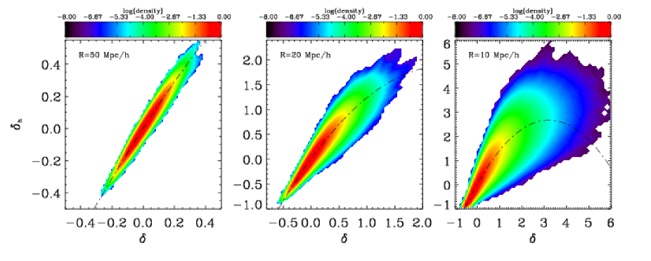
In Figure 1 we present the bin averaged scatter plots of vs. , averaged over the realizations. The colour contours are shaded by the normalized population density of that pixel, e.g. the central red region indicates that most of the points in the simulation are regions of density close to average. We also see that as the smoothing scale is decreased (panels going from left-to-right), that the scatter increases and that there are more points that have higher and lower density. Conversely, as the filter scale is increased the relation becomes tighter and more linear. One obvious conclusion that may be drawn from this behaviour is that the bias relation is certainly not deterministic.
| 50 | 1.3 0.1 | 1.497 0.002 | -0.577 0.031 |
|---|---|---|---|
| 20 | 12.0 0.1 | 1.542 0.006 | -0.635 0.004 |
| 10 | 37.2 0.1 | 1.644 0.005 | -0.512 0.001 |
In order to obtain a more quantitative understanding, we next consider fitting for the parameters of the local bias model at second-order. From Eq. (14) we have:
| (32) |
We perform a least-squares analysis on each realization, and then average over the resulting set of bias parameters to obtain the mean parameters: , , and . The -errors are then estimated in the usual way, as quadratic deviations from the sample mean. In Fig. 1 we plot the resultant best-fit local model as the dot-dashed line in each of the three panels.
The information on the parameters is summarized in Table 1 as a function of the filter scale . This clearly shows that the estimates of increase as the smoothing scale is decreased, whereas those for appear to be parabolical. Naively, one might expect that the nonlinear bias terms should approach zero as the amount of smoothing is increased and nonlinearities are washed out, however, at even with , the fluctuations are still significant enough to yield a non-zero . Note also that in all cases .
The local model, as written in Eq. (14), asserts that the parameters are independent of the smoothing scale , and we, therefore, consider the implications as follows. Suppose that nonlinear bias is exactly as described by Eq. (32), but that the coefficients are not independent of the smoothing scale. Let us now consider the results that would be obtained from measurements for two smoothing scales and . From Eq. (32) we would have:
| (33) | |||||
| (34) |
Supposing now that we desmoothed each of the fields, by Fourier transforming and dividing out the appropriate window function. We would then have:
In order for the above equations to be equivalent, then we must have
| (35) | |||||
| (36) |
The last of the two equations may only be satisfied if and only if or . Since the vs. method is inherently a real space measure it involves contributions from all Fourier modes. It is therefore difficult to ensure that .
We conclude that the above method will not be a safe way to recover bias parameters independent of the smoothing scale. We now turn to Fourier space methods.
| 0.03-0.09 | 1.589 0.002 | 1.493 0.002 | 1.589 0.004 | 1.487 0.004 |
|---|---|---|---|---|
| 0.04-0.12 | 1.624 0.002 | 1.486 0.002 | 1.638 0.003 | 1.489 0.003 |
| 0.05-0.15 | 1.663 0.002 | 1.474 0.002 | 1.709 0.003 | 1.503 0.003 |
| 0.06-0.18 | 1.695 0.001 | 1.460 0.002 | 1.775 0.002 | 1.511 0.003 |
4.2 Effective large-scale bias from power spectra
We now use various halo power spectra to derive estimates for an effective large-scale halo bias.
In order to do this, we first measure the Fourier transform of the matter and halo density fields as described in Appendix A. The halo-halo, halo-mass and mass-mass power spectra, , are then estimated from the data by performing the following sums:
| (37) |
where , is the sample volume (which in our case is the simulation volume), and where are the number of Fourier modes in a shell of thickness .
Following Smith et al. (2007), we next construct the estimators:
| (38) | |||
| (39) |
where is the number of simulations and is the linear matter power spectrum. Note that in the case of we also consider shot-noise corrected versions of these two estimators, i.e. we correct using Eq. (92). We denote these bias estimates by and , respectively. Finally, we determine the errors by evaluating the variance of each realization against the mean.
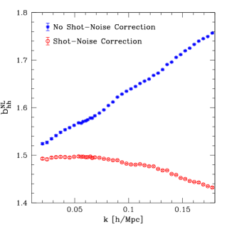
The first panel of Fig. 2 shows (solid blue data points) and (open red points). The bias for the shot-noise corrected terms remains roughly constant at down to scales and with very small errors, indicating that the result is highly constrained by the data. On scales smaller than this the bias is a decreasing function of . Without shot-noise correction, we find that the bias is strongly scale dependent, and the bias rapidly increases with increasing .
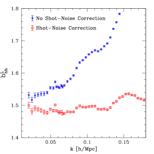
The second panel of Fig. 2 shows the results obtained from using (solid blue points) and (open hexagonal points). The results are similar to those for , but with increased cosmic variance on large scales. An oscillation structure is also present, this can be understood as explained in Guzik et al. (2007). Nevertheless, comparing the two provides a clear indication of the validity of the tree-level power spectrum up to .
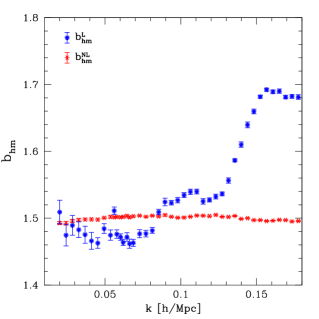
The third panel of Fig. 2 shows the bias results (solid red points) and (solid blue points). The value of stays roughly constant for the whole scale range considered in the estimate, while is not smooth and clearly shows the imprint of the oscillation structure. Nevertheless, we find , to within the errors for . On comparing the results for and , we see that for scales , these estimates are compatible and that the effective large-scale bias is roughly . Interestingly, these findings are consistent with real space measures of the effective large scale bias from cell variances (Smith & Marian, 2011).
In Table 2, we report the weighted average and corresponding 1 error on the effective bias, , computed over the same -modes corresponding to the magnitude of the third wavevector for each triangle configuration. The tabulated results for the analysis of the uncorrected data confirms the results shown in Figure 2, that bias is indeed scale-dependent. Applying the shot-noise correction yields a more constant effective bias, even for the range of -modes entering into our bispectrum estimation. Interestingly, the value found for , is in good agreement with the result for obtained from fitting the density fields smoothed on scales . Therefore, if we opt to infer that the effective bias is equivalent to over these scales, then the bispectrum (reduced bispectrum) should also yield this value for when fitted over the same scale ranges (c.f. Table 2). That is, if the local bias model is correct and the tree-level bispectrum (reduced bispectrum) is a sufficient description of the nonlinearities on these scales.
Before moving on, we point out that one can also use the halo power spectra to define an effective (Smith et al., 2009), however we shall not explore this here.
5 Halo bias from Bispectra
In this section, we present our main results from the analysis of the halo bispectra.
5.1 Bispectrum Estimation
The computational code used to estimate the matter and halo power and bispectra is a modified version of the code developed in Smith et al. (2008), which itself is based on the algorithm of Scoccimarro et al. (1998). The major modification to that code, which we have implemented, is that no random subsampling of the Fourier modes is performed to estimate the bispectrum. Instead, all modes that contribute to a particular triangle configuration are used. In this work we use a FFT grid of size to estimate the power and bispectra. We only evaluate triangles that have , but consider the variation of with the angular separation of the two vectors. The largest scale at which we estimate the bispectrum is , and this is , where . Further details of the bispectrum estimation procedure may be found in Appendix A.
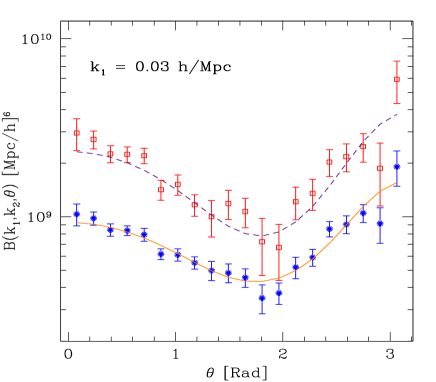
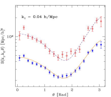
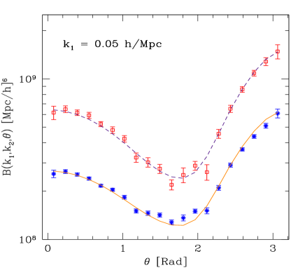
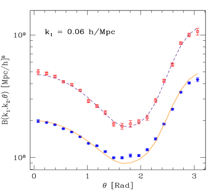
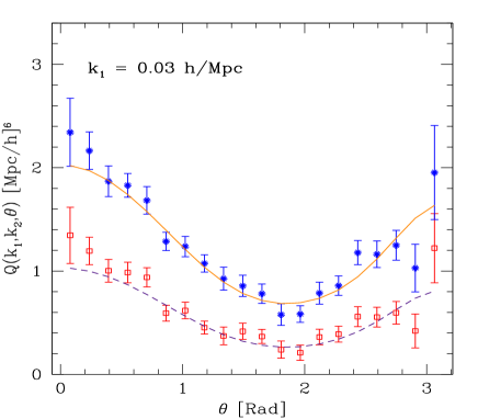
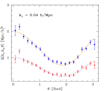
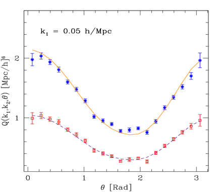
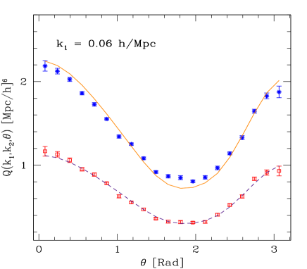
Figure 3 shows the ensemble-averaged shot-noise corrected results for the halo bispectra (open red squares) and matter bispectra (solid blue diamonds), measured from the ensemble of -body simulations. The four panels show the results obtained for the scales: . The error bars are the 1- errors on the mean, derived from the ensemble to ensemble variation. The solid red line represents the tree-level prediction for as given by Eq. (12). We see that this appears to be a good description of the estimates for the scales that we have considered. We notice that, for the case , the theory systematically under-predicts the measurements for (but see §5.4 for a more quantitative discussion of the goodness of fit).
5.2 Bias estimation
Our method for estimating the bias parameters follows an approach similar to that presented by Scoccimarro (2000) and Porciani & Giavalisco (2002). To start, we take a function that is a quadratic form of the type:
| (40) |
where is the number of angular bins considered and
| (41) |
Note that in dividing the difference between the estimate of the ensemble average bispectrum () and the model prediction () by the standard deviation (), is in fact the inverse correlation matrix. Recall that the correlation and covariance matrices are related by: .
In order to minimize this function and so recover the best-fit bias parameters, we need an estimate of , and we do this using the standard unbiased estimator:
| (42) |
where is the number of simulations and where
| (43) |
where in the above is the estimate of the bispectrum and where is the mean of the ensemble.
Next, we use singular-value-decomposition (SVD) to invert the . For the estimate of the inverse correlation matrix, we utilize principal component analysis (PCA) to remove some of the noisy eigenvectors. We select the fraction of principal components that account for 95% of the variance. According to this selection criteria we typically retain 15 out of 20 of the most ‘dominant’ eigenmodes. Note that as pointed out in Hartlap et al. (2007), . However, since we are using PCA, this should be a subdominant correction. Thus, we may approximate Eq. (40) as:
| (44) | |||||
where the correlation matrix was diagonalized by rotation into its eigenbasis, i.e. , with representing a diagonal matrix of eigenvalues. We also defined . Note that in the final approximate expression we include a matrix , this a diagonal matrix with entries either 1 or 0, depending on whether the eigenvector is to be retained or cut from the PCA reconstruction.
Finally, the function was minimized using the Levenberg-Marquardt routine for non-linear least squares fitting.
5.3 Errors in parameter estimates
To the best-fit parameters , we assign both systematic and statistical errors.
In our context, the systematic errors correspond to the errors induced in the best-fit parameters from fitting the data with a noisy inverse covariance matrix (or correlation matrix). Owing to the relatively low number of simulations , we expect that Eq. (42) provides a noisy estimate of . In order to estimate the errors this has on the best-fit parameters we employ the jackknife subsampling method (see for example Norberg et al., 2009). This involves slicing the total data set into subsamples. Then a resampling of the data is obtained by excluding one of the subsamples from the set. From this resampling we then estimate the mean statistic of interest and the inverse correlation matrix as described in the previous section. The resampled data set is then used to determine a new estimate of the best-fit bias parameters. This procedure is then repeated for all of the possible resamplings of the data. In our particular case we treat the measurements from each simulation as the regions to be included or excluded, and this gives us 40 jackknife estimates of the bias parameters . The parameter covariance matrix for the systematic errors can be computed as (Norberg et al., 2009):
| (45) |
where is the estimate of from the resampling of the data and is the estimate of the mean obtained from all of the resamplings.
The statistical error is obtained directly from the nonlinear least-squares analysis. The routine mrqmin provides an approximation to the errors on the parameters that corresponds to a for a one-parameter model. However, the confidence regions we present in the forthcoming plots correspond to either , which roughly denote the (, ) errors for a two-parameter model.
Given that we consider the two forms of error: systematic and statistical), and that one is never consistently larger than the other, in all forthcoming tables, we choose to report only the total error. This is obtained simply from the two errors added in quadrature.
5.4 Testing the validity of the tree-level matter
Before we report the estimates of the halo bias parameters, we first present a test of the validity of the tree-level model for the matter bispectrum. We do this by applying the test described above, to the and data, and so fit for and . Note that since the total number of principal components retained equals 15, then for a two-parameter model the number of degrees-of-freedom equals 13. If the tree-level expressions in the large-scale limit as given by Eqs (26) and (30) are correct, then we should expect to find and .
Table 3 presents the best-fit nonlinear bias parameters for the four different bispectrum scale ranges discussed earlier. In the analysis we fit the shot-noise corrected bispectra. The values (end column of the table), confirms that the tree-level expressions and , provide good fits for the triangle configurations with . However, for the fits are poor given the estimates, and we see that, for both and , they yield non-zero values for at 1. The results also imply that the failure of the tree-level model on these scales is more severe for than for . This can be understood by noting that from shows a prominent departure from unity, whereas does not (although the deviation still exceeds 2). We thus conclude that it is likely that the tree-level expressions for the halo bispectra will only be valid for , for our chosen bispectra configurations.
| 0.03 | 1.01 0.07 | -0.04 0.25 | 19.08 | |
| 0.93 0.19 | -0.05 0.30 | 19.03 | ||
| 0.04 | 0.98 0.03 | 0.04 0.10 | 14.31 | |
| 1.05 0.09 | 0.07 0.16 | 14.95 | ||
| 0.05 | 0.97 0.02 | 0.13 0.08 | 38.83 | |
| 1.14 0.07 | 0.19 0.13 | 19.97 | ||
| 0.06 | 0.98 0.02 | 0.10 0.10 | 34.09 | |
| 1.15 0.04 | 0.22 0.08 | 29.58 |
5.5 Constraints on and from halo bispectra
Table 4 presents the best-fit nonlinear bias parameters and their respective 1 errors in quadrature, obtained from the analysis of and . Note that we present the results for both the uncorrected and shot-noise corrected measurements, indicated in the table by superscript ‘SC’. Table 4 also shows the value of these best-fit parameters as an indication of the goodness-of-fit.
In Figures 3 and 4 we also show the tree-level theoretical models for and (dashed lines), where the best-fit bias parameters from Table 4 have been used. These figures demonstrate that, at least by-eye, the tree-level models provide a reasonable description of the data. However a more detailed inspection of Table 4 reveals some important discrepancies.
For the case of fitting , the shot-noise correction is less important, as we see that the estimates of for all bispectra configurations with and without shot-noise corrections are consistent to within the errors, and have . However, shows systematic differences, being more negative if the correction is made, and for this we find that . On the other hand, for the case of , the results clearly show that the shot-noise subtraction has an important effect on the recovered values for the bias parameters. If the shot-noise is not corrected, then we see that the estimates for increase systematically as we go from triangle configurations with to . Whereas if it is corrected, then we find and to within the errors. On comparing the results from and we see that, whilst the values for disagree significantly, surprisingly those for remain consistent at the 1 level.
| 0.03 | 1.43 0.11 | -0.18 0.40 | 17.20 | |
| 1.42 0.11 | -0.36 0.38 | 17.08 | ||
| 2.09 0.55 | -0.12 0.76 | 16.08 | ||
| 1.75 0.47 | -0.39 0.56 | 16.66 | ||
| 0.04 | 1.41 0.08 | -0.05 0.26 | 26.92 | |
| 1.38 0.08 | -0.27 0.25 | 26.16 | ||
| 2.32 0.39 | 0.14 0.58 | 26.40 | ||
| 1.80 0.29 | -0.34 0.36 | 26.96 | ||
| 0.05 | 1.40 0.06 | 0.15 0.21 | 31.92 | |
| 1.38 0.05 | -0.25 0.15 | 12.63 | ||
| 2.66 0.26 | 0.57 0.42 | 11.53 | ||
| 1.90 0.19 | -0.30 0.22 | 11.60 | ||
| 0.06 | 1.41 0.05 | 0.19 0.24 | 63.64 | |
| 1.37 0.03 | -0.23 0.13 | 19.30 | ||
| 2.84 0.20 | 0.88 0.40 | 20.70 | ||
| 1.87 0.14 | -0.30 0.19 | 19.47 |
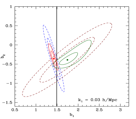
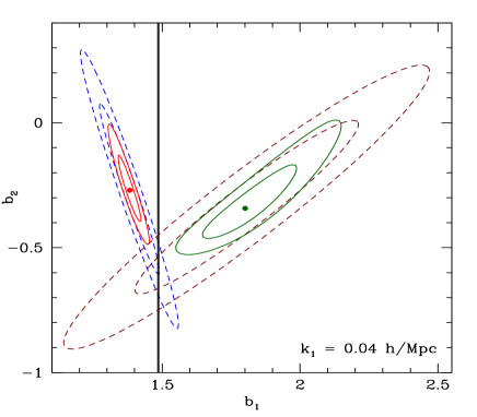
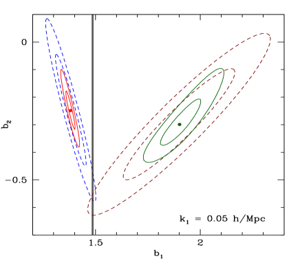
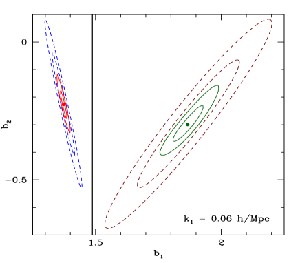
The function of Eq. (41) may be interpreted as a
Gaussian likelihood if we make the transformation, . Once suitably
normalized and on assuming a set of prior probabilities we may then
explore the shape of the confidence regions in the posterior probability
.
Figure 5 shows the 1 likelihood confidence contours in the posterior probability for the nonlinear bias parameters for the four scales considered according to our method of analysis described above. The solid lines denote the size of the confidence regions at the 68 and 95 level (i.e. ) when we construct a correlation matrix from the 40 realizations without regard for the systematic uncertainty. The dashed-lines demonstrate the magnitude at which the 68 and 95 confidence regions expand following our generation of a set of jackknife subsamples to monitor the effect due to the implicit error associated with the estimated correlation matrix. Hence, we clearly see the relevance of accounting for the uncertainty of the correlation matrix when obtaining the bias parameter constraints. The discrepancy between the resulting jackknife error ellipses for and is less severe than the likelihood contours obtained from the complete sample where the level of agreement improves progressing to large scales, yet this might be due to the fact that the statistical error is more prominent at larger scales. Interestingly, the overlap of the two likelihood regions at 2 for =0.03, 0.04 and 0.05 occurs with the rectangular region or strip denoting the effective bias measure, , at 1. These set of panels in Figure 5 convey pictorially the information obtained from the results in Table 4 that the likelihood contours from analysis of show an evolution with decreasing scale toward larger and larger , whereas the constraints on remain consistent. Lastly, the constraints obtained from analyzing the -amplitudes are much weaker than those coming from the bispectrum.
6 Halo bias from cross-bispectra
In §5.5 we saw that shot-noise corrections influenced the recovery of the bias parameters particularly for . In this section, we attempt to develop the use of cross-bispectra, as measures of the bias that are less susceptible to discreteness effects. The use of cross-correlations in large-scale structure work has long been known as a way of reducing discreteness corrections (Peebles, 1980). However, it is only relatively recent that it has been applied to study bias (Smith et al., 2007; Dalal et al., 2008; Smith, 2009; Padmanabhan et al., 2009; Desjacques et al., 2009; Pillepich et al., 2010).
6.1 Definitions and theory
We may define the halo cross-bispectra as follows:
| (46) | |||||
| (47) |
We then symmeterize these quantities by the operations:
| (48) | |||||
| (49) |
For ease of notation we shall now simply take and , unless otherwise indicated. We may now also define the cross-reduced bispectra as:
| (50) | |||||
| (51) |
where we have for the denominators (again symmetrized):
| (52) | |||||
| (53) | |||||
The relations for and can easily be constructed using a graphical approach. Let us consider three nodes two of which are the same and the third is different (we shall think of the nodes as the density fields). Label these nodes 1, 2, and 3. Now consider all possible ways to connect the three nodes together by two edges. When two nodes, which are the same, connect together this gives us an auto-power spectrum with a delta function, and when two nodes that are different connect together this gives us a cross-power spectrum and delta function. One may then symmetrize the results by considering all possible relabellings of the nodes and dividing by three.
In Appendix B we calculate the tree-level cross-bispectra, and , in the local model of halo biasing. The main results are:
| (54) | |||||
| (55) | |||||
In the limit of large scales, and or small smoothing scales, the filter functions and we have
| (56) | |||
At second order in the nonlinear bias and PT, the cross-reduced bispectra are:
| (58) | |||||
In the large-scale limit, , these expressions become:
| (60) | |||||
| (61) |
| 0.03 | 1.37 1.18 | -0.36 0.32 | 16.86 | |
| 1.37 1.18 | -0.36 0.32 | 16.86 | ||
| 1.98 0.75 | -0.75 0.99 | 19.09 | ||
| 1.98 0.75 | -0.75 0.99 | 19.09 | ||
| 0.04 | 1.33 0.16 | -0.33 0.51 | 16.83 | |
| 1.33 0.16 | -0.33 0.51 | 16.83 | ||
| 2.50 0.56 | -0.31 0.89 | 17.96 | ||
| 2.51 0.56 | -0.32 0.89 | 17.97 | ||
| 0.05 | 1.30 0.07 | -0.01 0.23 | 26.98 | |
| 1.30 0.07 | -0.02 0.23 | 26.82 | ||
| 2.94 0.25 | 0.24 0.57 | 16.90 | ||
| 2.94 0.25 | 0.23 0.57 | 16.95 | ||
| 0.06 | 1.29 0.07 | -0.001 0.28 | 13.99 | |
| 1.29 0.07 | -0.004 0.28 | 13.93 | ||
| 3.45 0.30 | 1.43 0.94 | 46.60 | ||
| 3.45 0.30 | 1.42 0.94 | 46.87 |
| 0.03 | 1.42 0.25 | -0.32 0.60 | 17.13 | |
| 1.42 0.24 | -0.45 0.47 | 17.49 | ||
| 2.08 0.40 | -0.49 0.46 | 17.45 | ||
| 2.11 0.40 | -0.67 0.42 | 17.46 | ||
| 0.04 | 1.39 0.14 | -0.24 0.25 | 21.29 | |
| 1.37 0.15 | -0.37 0.24 | 21.42 | ||
| 2.49 0.46 | -0.17 0.56 | 22.92 | ||
| 2.56 0.49 | -0.47 0.51 | 24.60 | ||
| 0.05 | 1.38 0.08 | -0.05 0.18 | 22.46 | |
| 1.36 0.07 | -0.29 0.14 | 13.16 | ||
| 2.87 0.18 | 0.22 0.29 | 12.55 | ||
| 2.92 0.19 | -0.37 0.25 | 16.77 | ||
| 0.06 | 1.39 0.07 | -0.07 0.25 | 20.56 | |
| 1.36 0.07 | -0.31 0.22 | 15.32 | ||
| 3.12 0.27 | 0.54 0.52 | 37.81 | ||
| 3.25 0.31 | -0.14 0.47 | 60.54 |
6.2 Estimation of the cross-bispectra
The cross-bispectra and can be estimated following the algorithm described in §5.1 with some small modifications. Firstly, the estimates must be symmetrized, and for the discrete form of we have,
| (62) | |||||
and with a similar relation for . The reduced bispectra are estimated by dividing the above bispectrum estimates by estimates for and from Eqs (52) and (53), respectively.
One further complication is constructing the corrections for shot-noise. This may be performed following the counts-in-cells approach of Peebles (1980) (and see also Smith, 2009). We find that the symmetrized corrections for and can be written as:
| (63) | |||||
| (64) |
where and , are the number density of matter particles and haloes, respectively. For the reduced bispectra we must correct the estimates of and , which are written in the following form:
| (65) | |||||
| (66) |
As it is the case that , we expect that the shot-noise corrections to will be significantly smaller than for . Hence, we shall think of this as being an almost perfect measure independent of discreteness.
Using these estimators, we compute the ensemble average and ensemble-to-ensemble variations of the halo-mass cross-bispectra. We do this for the same bispectra configurations that were considered in §5.1.
6.3 Nonlinear bias from cross-bispectra
We estimate the nonlinear bias parameters and their errors from the cross-bispectra using the same method employed for the auto-bispectra in §5.2 and §5.3. The results are tabulated in Tables 5 and 6, respectively.
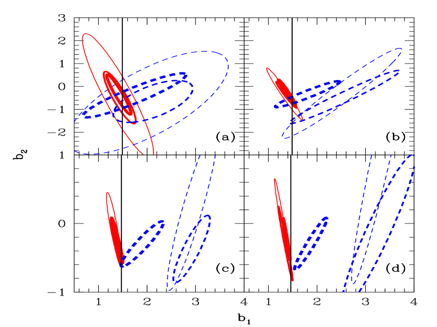
Figure 6 presents the 2-D 95% confidence likelihood contours for and , that are obtained from fitting the shot-noise corrected bispectra and reduced bispectra . The four panels show the results obtained from fitting triangle configurations, , with , and these correspond to the top-left, top-right, bottom left and bottom right panels, respectively. For comparative purposes, the vertical band in each panel, denotes the 1 constraint on , obtained from the shot-noise corrected halo and nonlinear matter power spectra (c.f. §4.2).
Consider first the bispectra (solid red lines of increasing thickness), from the figure and the tables, we see that all of the results are reasonably consistent with one another over the various scale ranges considered. However, when smaller scales are used (i.e. ), the consistency weakens and the best-fit parameters, obtained from and , differ by .
Evaluating the results for the reduced bispectra (dashed blue lines of increasing thickness), the four panels show a strong evolution of the error ellipses with scale. We also note that the level of agreement between the different estimators also evolves strongly, becoming weaker and weaker as smaller scales are considered. At the largest scale where , all of the 2 likelihood contour regions overlap. However, this consistency is broken for the next scale range, , where and are shifted downwards and further to the right favoring a more negative and higher . The trend continues in this same direction heading to smaller and smaller scales.
Comparing the results from both and together, we see that only on the largest scales is there any degree of overall consistency. One way to interpret the results up to now, is that, if we believe , then the agent driving the inconsistency between the parameter estimates, is the breakdown of the local bias model at tree-level. Furthermore, the breakdown of the local tree-level model is more severe for the reduced bispectrum than for the bispectrum.
7 The need for beyond tree level bias models
This final set of analysis consists of a simple proof of method test, and we determine whether, when the underlying bias model is known, the ‘true’ bias parameters of the model are indeed recoverable with our approach.
7.1 Biasing by hand
For these tests, and for simplicity, we shall assume that the local model of biasing at quadratic order is the correct underlying bias model. Nonlinear biased density fields of this type may be obtained through the following procedure.
For each of the outputs of the 40 simulations, we assign the nonlinear density field of matter to a cubical Fourier grid using the CIC algorithm. This is then Fourier transformed. Each Fourier mode is then smoothed using a Gaussian filter of scale . We then inverse Fourier transform this field and obtain the smoothed, nonlinear matter distribution in real space. Using this we next form the sum,
| (67) |
where and are the artificial bias parameters. Finally, this is Fourier transformed to give us . Thus, given and , we can now use our standard bispectrum estimators to estimate , , and . We refer to this procedure as the ‘biasing-by-hand’ test.
The major benefits of these tests are that we are able to better gauge the effects to which nonlinearities beyond tree-level order influence the measured bispectra and reduced bispectra. We also note that shot-noise plays no rôle here, since the biased field is created from the matter density field which is densely sampled.
7.2 Theoretical interpretation
In order to interpret the results from such a construction we may use the results presented in Appendix B, with the small modification that we do not de-smooth the results. If we define the smoothed bispectra as
| (68) |
then for , we have:
| (69) | |||||
| (70) | |||||
where for ease of notation we take and in the above we have suppressed the dependence of , , and , on . We have also introduced the auxiliary functions:
| (72) | |||||
| (73) | |||||
| (74) | |||||
| (75) | |||||
The attractive aspect of this test can now be understood: if we move the terms in Eqns (69), (70) and (LABEL:eq:bbb), which are proportional to from the right to the left-hand-side, then we may rewrite this system as the matrix equation:
| (76) |
where we defined , etc. This equation may be inverted to give,
| (77) |
Hence, if we specify , and measure the four bispectra , , and , then we can determine exactly , and . Thus we have complete knowledge of all components of the nonlinear model at all orders in the theory. The lowest order perturbation theory expansions of these statistics are (c.f. Appendix B):
| (78) | |||||
| (79) | |||||
| (80) |
where in the above, we defined .
| 20 | 1.62 0.07 | -0.46 0.12 | 0.01 | |
| 20 | 1.62 0.10 | -0.49 0.19 | 0.00 | |
| 20 | 1.63 0.22 | -0.53 0.51 | 0.00 | |
| 10 | 1.62 0.04 | -0.42 0.04 | 0.15 | |
| 10 | 1.62 0.06 | -0.47 0.07 | 0.02 | |
| 10 | 1.63 0.13 | -0.53 0.20 | 0.00 | |
| 6.7 | 1.59 0.04 | -0.35 0.02 | 0.70 | |
| 6.7 | 1.60 0.05 | -0.42 0.04 | 0.14 | |
| 6.7 | 1.63 0.12 | -0.53 0.12 | 0.00 |
| 20 | 1.63 0.11 | -0.67 0.36 | 14.75 | |
| 20 | 1.58 0.17 | -0.45 0.65 | 15.71 | |
| 20 | 1.37 0.33 | 0.56 1.19 | 18.43 | |
| 10 | 1.49 0.03 | -0.66 0.08 | 13.32 | |
| 10 | 1.48 0.04 | -0.69 0.13 | 13.60 | |
| 10 | 1.46 0.09 | -0.69 0.29 | 14.13 | |
| 6.7 | 1.36 0.02 | -0.74 0.06 | 13.21 | |
| 6.7 | 1.36 0.03 | -0.82 0.09 | 12.87 | |
| 6.7 | 1.32 0.07 | -0.86 0.22 | 13.13 |
7.3 Results of the artificial bias test
Following the algorithm described in §7.1, for each realization of our ensemble of simulations, we generate three artificially biased density fields smoothed on scales: . In all cases we apply the same nonlinear bias: and . Whilst these values are somewhat arbitrary, they were selected to coincide with the best-fit values to the scatter plot of vs. , smoothed at , that we recorded in §4.1.
For each filtering scale, we then measure the four bispectra , , and for triangle configurations with , , over 20 angular bins. From these we use the method described above, to recover the higher-order terms: , and .
We now define three modelling cases of interest:
- •
- •
- •
For each of the models described above, we then apply the same –fitting analysis, as described in §5.2 to determine the best-fit and parameters.
We begin by first examining the All Order expansion model. We confirm that for this case, the true bias parameters and are recovered exactly, albeit with some uncertainty, however, with a , and for all the smoothing lengths considered. This null test is important, because it gives us confidence that any departures of the fits from the true bias values, can be attributed solely to a break down of the theoretical modelling.
Next we focus on the Exact Trispectrum model where and are measured from the simulations. In Table 8 we report the best-fitting bias parameters with the 1 errors expressed in quadrature for the auto- and cross-bispectrum and for the four smoothing scales examined. For the case , a quick inspection of Eq. (69) tells us that the modelling should be exact, and indeed we see that the bias parameters are correctly recovered. However, for the cases and we see that the absence of the higher-order terms (), induce biases in the parameters. For the deviation from the true value is relatively small, with the value of the parameter only slightly decreasing in size. For the deviations are larger, and this parameter becomes more positive. We also note that the deviations from the true values appear to increase as the smoothing scale is decreased.
Finally, we focus on the Tree-level model. Table 8 presents the best-fit results for and . We see that in nearly all cases, there are systematic biases in the recovery of the nonlinear bias parameters for all of the measured bispectra. In particular, for the case of , the results are most deviant and poorly constrained. Whereas for , only when the data has been smoothed on scales are the recovered parameters close to the true values.
The comparison of the results from this analysis leads us to conclude that the recovered bias parameters are very sensitive to the inclusion of beyond leading order corrections in the modelling. Furthermore, accurate nonlinear modelling of, at the very least, the matter bispectrum and trispectrum will be essential, if we are to safely recover the nonlinear bias parameters from this approach.
8 Discussion
We have evaluated the local halo bias model at second-order using three different probes: smoothed density fields; power spectra; and bispectra and reduced bispectra. A summary of our results for the best-fitting bias parameters determined from shot-noise corrected spectra is shown in Figure 7.
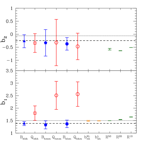
In the figure we also compare our estimates for and with the analytical predictions for the halo bias parameters obtained from the peak background split (PBS) ansatz (Bardeen et al., 1986; Mo & White, 1996). The average theory bias parameters are obtained through computing the expression:
| (81) |
where is the halo mass function, and is set equal to the value of the minimum halo mass identified in the simulations (see §3) . We evaluate the above integral using three different fits to N-body simulations by Sheth & Tormen (1999), Warren et al. (2006) and Pillepich et al. (2010). The corresponding expressions for the bias parameters as a function of halo mass are presented in Scoccimarro et al. (2001) and Manera et al. (2010).
Considering, the results for (bottom panel), we see that when the reduced bispectra, , and are used, the recovered parameters are poorly constrained and appear incompatible with respect to the other estimates and are only weakly consistent with one another. On the other hand, the estimates from the bispectra , and are in much better agreement with each other. They are also in close agreement with the predictions from Warren et al. (2006) and Pillepich et al. (2010), which both provided an estimate of . However, they slightly undershoot the values from the effective bias estimates, and , likewise the smoothed density fields, and the Sheth-Tormen prediction. The analytical predictions from the Sheth & Tormen (1999) mass-function yielded in good agreement with the power spectrum and density field results smoothed on a scale . The recovered values of from the effective bias in the power spectra and the smoothed density fields collectively are in broad agreement, but the latter increase with decreasing smoothing scale.
In the top panel of the figure, we see that the constraints on from the different estimators used in the simulations are reasonably consistent with one another, albeit with significant error bars. These estimates also agree well with the PBS prediction from the Warren et al. (2006) and Pillepich et al. (2010) mass functions, which give an average . However, the prediction from the Sheth & Tormen (1999) mass function gives , and this appears to be in worse agreement with the data.
There are a number of possible explanations for the deviations in the recovered bias parameters. Firstly, the relation between matter and halo fluctuations may not be local. Indeed, we know it is not deterministic owing to the scatter in relation vs. . Perhaps, this is a consequence of non-locality. In this case we need a more advanced theoretical approach to understand the halo clustering. One possibility may be that the bias is local in Lagrangian space (Catelan et al., 2000; Matsubara, 2011).
Secondly, our simple biasing-by-hand test has enabled us to discern that, for the current set of tests that we have performed, the most likely explanation at this point is that the tree-level expansions for and are not sufficiently accurate enough. Higher-order nonlinear corrections in the modelling must be included, and if possible all order expansions for and would be invaluable.
Thirdly, as we have argued, the local bias model only makes sense in the context of smoothing. The bias parameters one recovers from fitting, depend sensitively on the smoothing scale . For the biasing-by-hand tests, the exact smoothing scale was known beforehand. However, in real data we do not know this a priori. In all of the cases, when recovering bias parameters from the bispectra, we have assumed that we are on sufficiently large scales such that . However, in general should be a free parameter and as such, marginalized over in the analysis.
Manera & Gaztañaga (2011) performed a similar study of nonlinear halo bias with the three-point correlation function in configuration space. In contrast to our analysis, they measured the bias parameters for different halo mass bins. They found inconsistencies between the predictions of the different estimators considered. They evaluated the scatter plots of vs. as function of smoothing scale, and found that stability in the local bias parameters ( occurred for smoothing scales, , albeit with larger errors. They also found that the bias predictions derived from vs. for were in good agreement, to within the errors, with the linear bias measured from evaluating the two-point correlation function on large and intermediate scales. As in the case of our findings, they found the linear bias measured from evaluating the three-point correlation function, expressed in terms of the -amplitudes, was not consistent with that of the two-point correlation function for the lower mass bins: . They were unable to formulate solid conclusions for larger mass ranges.
Guo & Jing (2009) explored the differences between estimates of bias from and . They also found that based on analysis of the mock galaxy catalogues was larger for galaxy reduced bispectra and power spectra than for . While Guo & Jing (2009) also noted that this might be due to the failure of SPT at tree-level, they also reported that agreement could be found between estimators if measured directly from the simulations was used in place of the tree-level expression. However, when we performed the same test with our data we found no dramatic reconciliation of the two bias estimates. The investigation performed by Guo & Jing (2009) was carried out using only 4 large volume and 3 smaller volume runs. As a result of having too few realizations, they assumed the Gaussian approximation for the covariance matrix in order to perform their study at large-scales.
9 Conclusions
In this paper we have used a sample of 40 large volume -body simulations, with total volume , to test the local model of halo biasing, and the extent to which nonlinearities impact the modelling. We used three different methods for exploring the bias: smoothed density fields; power spectra; and bispectra and reduced bispectra. We focused mainly on the results from the bispectra. All of the reported results were scaled to a single realization of our simulations, and so are directly relevant for galaxy surveys with a total volume .
In §2 we reviewed the basic results of perturbation theory and how they connect to density statistics. We then reviewed the local model of halo biasing, drawing special attention to the rôle that smoothing plays in the theory. The important result being that even at tree-level, the smoothing explicitly enters the theory. The expressions for and , which are typically used in all past and current analysis, make the assumption that smoothing is unimportant. In subsequent sections we argued that this assumption is not safe.
In §3 we described our suite of -body simulations, and the halo catalogues used in this study.
In §4 we made measurements of the relation between and smoothed on the set of scales . To this data we fitted the local model of halo biasing up to second order, including , and . We found that the fits were reasonably good, however the best-fit parameters showed a running with the filter scale . We then demonstrated, theoretically, why the nonlinear bias parameters from this approach, could not be made independent of smoothing scale. We then turned to Fourier space statistics, and used the halo auto- and cross-power spectra to obtain an effective large-scale bias. We found that the effective bias estimators and were reasonably scale independent for . However, on scales smaller than this, decreased with increasing wavenumber, whereas remained surprisingly flat.
In §5 we estimated the matter auto- and halo auto-bispectra and reduced bispectra from our simulations. We measured these statistics for the triangle configurations and with and . These triangles all lay in the weakly nonlinear regime . We modeled these estimates using tree-level perturbation theory expressions for the matter bispectrum and nonlinear bias at second order, and assumed smoothing to be unimportant. Our method for estimation of the bias parameters followed a standard minimum approach. We estimated the covariance matrix for the full ensemble applying principal component analysis to minimize the intrinsic noise. We also performed a jackknife subsampling routine to propagate the error of the estimated covariance matrix onto the errors of the bias parameters.
We tested how well the measurements of the matter bispectra and reduced bispectra could be described by such modelling. The results obtained for the bias parameters and showed that the tree-level expressions were a good description of the data for configurations, , for which and . However, for smaller scale triangles, , significant deviations were apparent, and these were manifest as and at high significance.
We then applied the test to the halo bispectra and reduced bispectra . We found, for the shot-noise corrected , that the estimated values for and were reasonably consistent with one another. However, the fits became progressively poorer as smaller scales were added, yet the reduced– remained for . For the shot-noise corrected , we found that the values of were significantly larger , with large errors, and the values evolved with triangle configuration scale. However, , appeared to be more stable, although again with large errors. For triangle configurations with , the fits from and were inconsistent with each other at the level. For both and shot-noise corrections significantly influenced the recovered bias parameters.
In §6 we explored the halo and matter cross-bispectra, and , and reduced bispectra and . We calculated the tree-level expressions for these quantities symmetrized in all of their arguments. We then developed estimators for them. We showed that for and , provided the matter distribution was densely sampled, the shot-noise corrections were small.
We applied the analysis from §5 to these statistics and recovered the best-fit values for and . We found that for the shot-noise corrected data were all reasonably consistent with one another, giving and . For we found a similar pattern, except that for where we found , but with large errors. The results for and appeared to vary significantly.
Finally in §7 we explored to what extent the break-down could be attributed to the absence of terms that were beyond tree-level in the modelling. In order to do this, we developed a novel approach, whereby we constructed smoothed biased density fields from the smoothed matter density field, using the local model at quadratic order. We showed that if we set and to some fiducial values, and then measured the smoothed matter and halo bispectra and their cross-bispectra, then the higher order matter correlators , and could be recovered exactly. Thus we were able to construct three models: an all order model; a model that used the exact matter bispectrum and trispectrum; and a tree-level model.
We applied the analysis using these three models and for bispectra with . As expected, the exact model recovered the correct bias parameters. The model with the exact and , was in fact also exact for . For and the recovered parameters were close to the true values, but showed evolution with smoothing scale. Finally, for the tree-level model we showed that there was a significant evolution in the estimated bias parameters with smoothing scale and with the type of statistic used.
We conclude that estimates of nonlinear bias from the bispectrum that do not attempt to account for higher-order corrections, will most likely provide biased estimates for the bias parameters and . Robust modelling of nonlinear bias from bispectra, will, at the very least, require almost exact models for the matter bispectrum and trispectrum.
Real space estimates of bias appear to be inconsistent with Fourier space based ones. We believe that this owes primarily to the mixing of large- and small-scale wavemodes in real space. We therefore recommend that perturbative methods should strictly be applied in Fourier space. We also recommend that measurements focus on the bispectrum and the associated cross statistics, rather than the reduced bispectra, since this appears very sensitive to nonlinearities in the modelling and also shot-noise corrections.
Finally, we emphasize the importance of smoothing in the local model. Owing to the fact that the smoothing scale associated with the halo/galaxy distribution in question is not known a priori, it must be treated as a nuisance parameter and so marginalized over.
An alternative strategy for recovering information from higher order statistics, which may be of interest for future consideration, is the use of ‘Gaussianizing transformations’ or ‘density clipping’ (Neyrinck et al., 2009; Seo et al., 2011; Simpson et al., 2011). However, the theoretical connection between what is measured and what is interpreted from such approaches still remains to be fully calculated.
Acknowledgements
We thank the anonymous referee for helpful suggestions. We also thank Tobias Baldauf, Martin Crocce, Roman Scoccimarro, Emiliano Sefussati, Ravi Sheth and Masahiro Takada for useful discussions. We thank V. Springel for making public GADGET-2 and for providing his B-FoF halo finder, and R. Scoccimarro for making public his 2LPT code. JEP and CP were supported by funding provided through the SFB-Transregio 33 “The Dark Universe” by the Deutsche Forschungsgemeinschaft. RES acknowledges support from a Marie Curie Reintegration Grant, the Alexander von Humboldt Foundation and partial support from the Swiss National Foundation under contract 200021-116696/1.
References
- Baldauf et al. (2011) Baldauf T., Seljak U., Senatore L., 2011, Journal of Cosmology and Astro-Particle Physics, 4, 6
- Bardeen et al. (1986) Bardeen J. M., Bond J. R., Kaiser N., Szalay A. S., 1986, ApJ, 304, 15
- Bernardeau et al. (2002) Bernardeau F., Colombi S., Gaztañaga E., Scoccimarro R., 2002, Phys. Rep. , 367, 1
- Bouchet et al. (1995) Bouchet F. R., Colombi S., Hivon E., Juszkiewicz R., 1995, A&A, 296, 575
- Catelan et al. (2000) Catelan P., Porciani C., Kamionkowski M., 2000, MNRAS, 318, L39
- Coles (1993) Coles P., 1993, MNRAS, 262, 1065
- Crocce et al. (2006) Crocce M., Pueblas S., Scoccimarro R., 2006, MNRAS, 373, 369
- Dalal et al. (2008) Dalal N., Doré O., Huterer D., Shirokov A., 2008, PRD, 77, 123514
- Davis et al. (1985) Davis M., Efstathiou G., Frenk C. S., White S. D. M., 1985, ApJ, 292, 371
- Dekel & Lahav (1999) Dekel A., Lahav O., 1999, ApJ, 520, 24
- Dekel & Rees (1987) Dekel A., Rees M. J., 1987, Nature, 326, 455
- Desjacques et al. (2009) Desjacques V., Seljak U., Iliev I. T., 2009, MNRAS, 396, 85
- Feldman et al. (2001) Feldman H. A., Frieman J. A., Fry J. N., Scoccimarro R., 2001, Physical Review Letters, 86, 1434
- Fry (1994) Fry J. N., 1994, ApJ, 421, 21
- Fry & Gaztanaga (1993) Fry J. N., Gaztanaga E., 1993, ApJ, 413, 447
- Fry & Scherrer (1994) Fry J. N., Scherrer R. J., 1994, ApJ, 429, 36
- Gaztañaga et al. (2005) Gaztañaga E., Norberg P., Baugh C. M., Croton D. J., 2005, MNRAS, 364, 620
- Gaztañaga & Scoccimarro (2005) Gaztañaga E., Scoccimarro R., 2005, MNRAS, 361, 824
- Goroff et al. (1986) Goroff M. H., Grinstein B., Rey S.-J., Wise M. B., 1986, ApJ, 311, 6
- Guo & Jing (2009) Guo H., Jing Y. P., 2009, ApJ, 702, 425
- Guzik et al. (2007) Guzik J., Bernstein G., Smith R. E., 2007, MNRAS, 375, 1329
- Hartlap et al. (2007) Hartlap J., Simon P., Schneider P., 2007, A&A, 464, 399
- Heavens et al. (1998) Heavens A. F., Matarrese S., Verde L., 1998, MNRAS, 301, 797
- Hivon et al. (1995) Hivon E., Bouchet F. R., Colombi S., Juszkiewicz R., 1995, A&A, 298, 643
- Hockney & Eastwood (1988) Hockney R. W., Eastwood J. W., 1988, Computer simulation using particles. Bristol: Hilger, 1988
- Jain & Bertschinger (1994) Jain B., Bertschinger E., 1994, ApJ, 431, 495
- Jing (2005) Jing Y. P., 2005, ApJ, 620, 559
- Joachimi et al. (2009) Joachimi B., Shi X., Schneider P., 2009, A&A, 508, 1193
- Juszkiewicz (1981) Juszkiewicz R., 1981, MNRAS, 197, 931
- Kaiser (1984) Kaiser N., 1984, ApJL, 284, L9
- Komatsu et al. (2010) Komatsu E., The WMAP Team 2010, ArXiv e-prints
- Komatsu et al. (2009) Komatsu E., Dunkley J., Nolta M. R., Bennett C. L., Gold B., Hinshaw G., Jarosik N., Larson D., Limon M., Page L., Spergel D. N., Halpern M., Hill R. S., Kogut A., Meyer S. S., Tucker G. S., Weiland J. L., Wollack E., Wright E. L., 2009, ApJS, 180, 330
- Makino et al. (1992) Makino N., Sasaki M., Suto Y., 1992, PRD, 46, 585
- Manera & Gaztañaga (2011) Manera M., Gaztañaga E., 2011, MNRAS, 415, 383
- Manera et al. (2010) Manera M., Sheth R. K., Scoccimarro R., 2010, MNRAS, 402, 589
- Marin (2010) Marin F., 2010, ArXiv e-prints
- Matarrese et al. (1997) Matarrese S., Verde L., Heavens A. F., 1997, MNRAS, 290, 651
- Matsubara (2011) Matsubara T., 2011, PRD, 83, 083518
- McBride et al. (2011) McBride C. K., Connolly A. J., Gardner J. P., Scranton R., Newman J. A., Scoccimarro R., Zehavi I., Schneider D. P., 2011, ApJ, 726, 13
- Mo et al. (1997) Mo H. J., Jing Y. P., White S. D. M., 1997, MNRAS, 284, 189
- Mo & White (1996) Mo H. J., White S. D. M., 1996, MNRAS, 282, 347
- Neyrinck et al. (2009) Neyrinck M. C., Szapudi I., Szalay A. S., 2009, ApJL, 698, L90
- Nishimichi et al. (2007) Nishimichi T., Ohmuro H., Nakamichi M., Taruya A., Yahata K., Shirata A., Saito S., Nomura H., Yamamoto K., Suto Y., 2007, Publications of Astronomical Society of Japan, 59, 1049
- Nishimichi et al. (2010) Nishimichi T., Taruya A., Koyama K., Sabiu C., 2010, Journal of Cosmology and Astro-Particle Physics, 7, 2
- Norberg et al. (2009) Norberg P., Baugh C. M., Gaztañaga E., Croton D. J., 2009, MNRAS, 396, 19
- Padmanabhan et al. (2009) Padmanabhan N., White M., Norberg P., Porciani C., 2009, MNRAS, 397, 1862
- Peebles (1980) Peebles P. J. E., 1980, The large-scale structure of the universe. Research supported by the National Science Foundation. Princeton, N.J., Princeton University Press, 1980. 435 p.
- Peebles & Groth (1975) Peebles P. J. E., Groth E. J., 1975, ApJ, 196, 1
- Pillepich et al. (2010) Pillepich A., Porciani C., Hahn O., 2010, MNRAS, 402, 191
- Porciani & Giavalisco (2002) Porciani C., Giavalisco M., 2002, ApJ, 565, 24
- Roth & Porciani (2011) Roth N., Porciani C., 2011, MNRAS, 415, 829
- Scoccimarro (1998) Scoccimarro R., 1998, MNRAS, 299, 1097
- Scoccimarro (2000) Scoccimarro R., 2000, ApJ, 544, 597
- Scoccimarro et al. (1998) Scoccimarro R., Colombi S., Fry J. N., Frieman J. A., Hivon E., Melott A., 1998, ApJ, 496, 586
- Scoccimarro et al. (1999) Scoccimarro R., Couchman H. M. P., Frieman J. A., 1999, ApJ, 517, 531
- Scoccimarro et al. (2001) Scoccimarro R., Feldman H. A., Fry J. N., Frieman J. A., 2001, ApJ, 546, 652
- Scoccimarro et al. (2001) Scoccimarro R., Sheth R. K., Hui L., Jain B., 2001, ApJ, 546, 20
- Sefusatti (2009) Sefusatti E., 2009, PRD, 80, 123002
- Sefusatti et al. (2006) Sefusatti E., Crocce M., Pueblas S., Scoccimarro R., 2006, PRD, 74, 023522
- Sefusatti & Komatsu (2007) Sefusatti E., Komatsu E., 2007, PRD, 76, 083004
- Seljak et al. (2003) Seljak U., Sugiyama N., White M., Zaldarriaga M., 2003, PRD, 68, 083507
- Seljak & Zaldarriaga (1996) Seljak U., Zaldarriaga M., 1996, ApJ, 469, 437
- Seo et al. (2011) Seo H.-J., Sato M., Dodelson S., Jain B., Takada M., 2011, ApJL, 729, L11+
- Sheth & Lemson (1999) Sheth R. K., Lemson G., 1999, MNRAS, 304, 767
- Sheth & Tormen (1999) Sheth R. K., Tormen G., 1999, MNRAS, 308, 119
- Simpson et al. (2011) Simpson F., Berian James J., Heavens A. F., Heymans C., 2011, ArXiv e-prints
- Smith (2009) Smith R. E., 2009, MNRAS, pp 1337–+
- Smith et al. (2009) Smith R. E., Hernández-Monteagudo C., Seljak U., 2009, PRD, 80, 063528
- Smith & Marian (2011) Smith R. E., Marian L., 2011, MNRAS, p. 1484
- Smith et al. (2007) Smith R. E., Scoccimarro R., Sheth R. K., 2007, PRD, 75, 063512
- Smith et al. (2008) Smith R. E., Sheth R. K., Scoccimarro R., 2008, PRD, 78, 023523
- Springel (2005) Springel V., 2005, MNRAS, 364, 1105
- Verde et al. (2002) Verde L., Heavens A. F., Percival W. J., Matarrese S., The 2dFGRS Team 2002, MNRAS, 335, 432
- Vishniac (1983) Vishniac E. T., 1983, MNRAS, 203, 345
- Warren et al. (2006) Warren M. S., Abazajian K., Holz D. E., Teodoro L., 2006, ApJ, 646, 881
- White & Rees (1978) White S. D. M., Rees M. J., 1978, MNRAS, 183, 341
Appendix A Bispectrum Estimation: Algorithm
Briefly, the algorithm that we employ is as follows: firstly the dark matter density field is computed by assigning the dark matter particles to a cubical grid using the ‘Cloud in Cell’ (CIC) technique (Hockney & Eastwood, 1988). Next the fast Fourier transform (FFT) of the gridded density field is computed. Each Fourier mode is then corrected for convolution with the Fourier mesh. We do this by dividing out from each mode, the Fourier transform of the window assignment function of the CIC scheme (Hockney & Eastwood, 1988; Jing, 2005):
| (82) |
where subscript denotes gridded quantities, is the Nyquist frequency of the mesh and is the number of Fourier grid cells.
The estimator for the bispectrum can be written (Scoccimarro et al., 1998):
| (83) |
where is the sample volume (in our case the simulation volume), the normalization factor, , can be written as (Sefusatti et al., 2006; Joachimi et al., 2009)
| (84) |
and we write in shorthand . A practical implementation of the above estimator may be achieved through (Smith et al., 2008):
| (85) |
where superscript denotes discretized quantities; denotes an integer vector from the origin of the -space to each mesh point; represents a pair of integer vectors, which lie in thin shells centred on and and whose angular separation lies in a narrow angular bin centred on , and for which . The upper limit of the sum represents the total number of triangles that have such a configuration.
The estimator for the bin-averaged reduced bispectrum, , is written as:
| (86) |
where is the estimator for the bin-averaged cyclical terms of the power spectrum generated from first computing the bin-averaged power-spectra, . Note that we estimate the power spectra that enter into this product in a slightly different way than normal: we use only those modes that go into estimating the particular triangle configuration to estimate . Hence,
| (87) |
where and where is dependent on the angular bin, since, with and fixed, we still have and the closure criterion implies varies as function of . Therefore,
| (88) |
The estimates of and are then corrected for discreteness, i.e. shot-noise. For the estimators of interest, the corrections are (Peebles, 1980; Smith et al., 2008):
| (89) | |||||
| (90) | |||||
| (91) |
Shot-noise corrected estimates of the statistics are obtained:
| (92) |
where and where . Note that the above recipe corrects some typos that are present in Smith et al. (2008).
Appendix B Halo cross-bispectra in the local model
As was shown in Eq. (15), at quadratic order, the local model of nonlinear biasing can be written as:
| (93) |
where , is the filtered density. Using this model we may now proceed to calculate the halo auto- and halo-mass cross-bispectra.
B.1 Halo-mass-mass bispectrum in the local model
Let us start with the simplest three-point cross-statistic, the halo-matter-matter bispectrum, this can be written:
| (94) | |||||
Let us define the smoothed -point spectra as:
| (95) | |||||
where , , and where . We may now integrate over to obtain
| (96) |
On dividing the above expression by , then we find the halo-mass-mass bispectrum can be written as
| (97) |
We may symmetrize the above result by constructing the sum , and this gives us:
| (98) |
On expanding and to fourth order in , the above expression can be approximated as,
| (99) |
Finally, in the large-scale limit , or for arbitrarily small smoothing scales, , the above expression becomes,
| (100) |
The reduced bispectrum is given by
| (101) |
where
| (102) |
In order to calculate the reduced halo-mass cross-bispectrum, then we need to evaluate the halo-matter power spectrum. In the local model and up to quadratic order in the bias we have,
| (103) |
Using the above expression in Eq. (102) we find
| (104) | |||||
If we expand to fourth order in the density then the above expression simplifies to:
| (105) |
Hence we have,
| (106) |
Finally, in the limit that , and the above result can be approximated by
| (107) |
B.2 Halo-halo-mass bispectrum in the local model
Again, using Eq. (93), the halo-halo-mass bispectrum, symmetrized in the arguments, can be written:
| (108) | |||||
If we use perturbation theory to expand , , and , and only keep terms that are order in the density field, then the above expression can be approximated by:
| (109) |
In the large-scale limit , the above expression can be approximated as:
| (110) |
The reduced bispectrum is given by,
| (111) |
where
| (112) |
The halo-mass power spectrum is given by Eq. (103) and the halo auto-power spectrum is given by:
| (113) | |||||
Expanding the above expression to lowest order in perturbation theory gives,
| (114) |
Using the above expression, we find that the tree-level expression for the reduced bispectrum can be written:
| (115) |
In the large-scale limit , we again have and
| (116) |
B.3 Halo-halo-halo bispectrum in the local model
Again using Eq. (93), the halo-halo-halo bispectrum, symmetrized in the arguments, can be written:
If we use perturbation theory to expand , , , , and , and keep only terms that are fourth order in the density field, then the above expression can be approximated by:
| (118) |
In the large-scale limit , the above expression can be approximated as:
| (119) |
The reduced halo-halo-halo bispectrum is given by,
| (120) |
where
| (121) |
where the halo auto-power spectrum is given by Eq. (113). On expanding the above expression to fourth order in the density we find,
| (122) |
Using the above expression, we find that the tree-level expression for the reduced bispectrum can be written:
| (123) |
In the large-scale limit , we again have and
| (124) |