Dynamic mean-field and cavity methods for diluted Ising systems

Erik Aurell Department of Computational Biology, AlbaNova University Centre, 106 91 Stockholm, Sweden Department of Information and Computer Science, Aalto University, Finland ACCESS Linnaeus Centre, KTH - Royal Institute of Technology, Stockholm, Sweden    Hamed Mahmoudi Department of Information and Computer Science, Aalto University, Finland
Abstract

We compare dynamic mean-field and dynamic cavity as methods to describe the stationary states of dilute kinetic Ising models. We compute dynamic mean-field theory by expanding in interaction strength to third order, and compare to the exact dynamic mean-field theory for fully asymmetric networks. We show that in diluted networks the dynamic cavity method generally predicts magnetizations of individual spins better than both first order (“naive”) and second order (“TAP”) dynamic mean field theory.

pacs:
64.60.-i, 68.43.De, 75.10.Nr, 24.10.Ht

I Introduction

(Classical) statistical mechanical systems in equilibrium are described by the Gibbs measure, which connects the propensity of a system to move between two states taken in isolation (the energy differences between these two states) to the probability of finding the system in one of the states, when all states are available. This relation is normally used to find equilibrium statistics of a system (magnetizations, correlation functions etc.) by sampling a dynamics for which the Gibbs measure in a stationary state. A Markov Chain Monte Carlo (MCMC) method, such as Glauber dynamics for Ising systems, which we will review briefly below in Sec. II, can work if the sample average converges quickly enough to Gibbs measure, and if the quantity to be measured has wide support in phase space. Well-known scenarios where this is case are spin systems in the high-temperature phase and when measuring e.g. total magnetization. In the low-temperature phase relaxation time to the Gibbs distribution can be very long. On the other hand, if the quantity to be measured is e.g. the magnetization of a single spin, then MCMC in a large system is slow for the trivial reason that one needs to sweep through all the spins while just being interested in the changes in and average over one of them. If the interactions are weak, marginal probability distributions can be computed perturbatively in mean-field theory Thouless et al. (1977); Parisi (1988); Tanaka (2000), which give closed equations for e.g. single-spin magnetizations. For dilute systems, where every spin is not connected to most other spins, very powerful message-passing methods have been developed by physicists, information theorists and computer scientists over the last two decades to compute marginals of Gibbs distributions quickly and accurately Yedidia et al. (2003); Mézard and Montanari (2009). While these cavity equations cannot (in their simplest form) deal with the complex phases of random spin systems at low temperature, in suitable scenarios they are much more accurate than mean-field theory, and they greatly improve on MCMC for single site magnetization and other local properties by substituting a cumbersome sampling by a direct deterministic computation. The cavity method has found to have many technological as well as fundamental applications Pearl (1988, 2000); Opper and Winther (2001); Kschischang et al. (1998); Mézard and Montanari (2009).

The situation is very different for out-of-equilibrium systems, in itself is an extremely broad term covering everything from macroscopic hydrodynamics (turbulence) Frisch (1995) and physical and chemical kinetics van Kampen (2007) to interdisciplinary applications of statistical physics to neuroscience, population biology, and other fields Hopfield (1982); Blythe and McKane (2007). We here consider the model systems obtained when generalizing the MCMC rules of Ising spin systems (Glauber dynamics) from the equilibrium case (symmetric interactions) to a non-equilibrium case (non-symmetric interactions). Such “kinetic Ising” models are only conceptual – but tractable – models of real spin systems driven out of equilibrium, and have mainly been studied with applications to neuroscience in mind Derrida et al. (1987); Hertz et al. (1986, 1987); Crisanti and Sompolinsky (1988). From the mathematical point of view, they are specific examples of Markov chains which do not obey detailed balance conditions. In contrast to equilibrium systems, there is hence no simple expression for a stationary state akin to a Gibbs measure, but such a state, when it exists, is a (complicated) function of all the details of the model. On the other hand, MCMC works as well in such systems as for standard equilibrium Ising models, and mean-field theory have been developed up to second order in the interaction strength Kappen and Spanjers (2000). This leaves open the case of dilute kinetic Ising models, where in the equilibrium case cavity methods would be preferable. A dynamic cavity method has only very recently developed for majority dynamicsKanoria and Montanari (2011) and Glauber dynamics Neri and Bollé (2009) and was investigated by us for parallel and sequential update schemes in Aurell and Mahmoudi (2011a).

The dynamic cavity method as outlined in Aurell and Mahmoudi (2011a) comprises first an ansatz on probability distributions, similar to standard cavity, then the Belief Propagation ansatz that cavity distributions factorize, and then also a further assumption of Markovianity. As discussed in Aurell and Mahmoudi (2011b), the second assumption is exact for fully asymmetric models with the parallel update rule. In a more general case, where either the interaction matrix has both a symmetric and an asymmetric component, or where the update rule is different, it is however but an approximation. The numerical results of Aurell and Mahmoudi (2011a), which showed that for some such mixed instances the dynamic cavity is quite accurate, were somewhat unexpected. The main motivation for the present paper is therefore to show more systematically in what parameter ranges dynamic cavity converges (for these models), where it is accurate compared to MCMC, and to compare its predictions to mean field theory. We will show that for dilute kinetic Ising models, dynamic cavity works also for the magnetizations of individual spins, and is considerably more accurate than mean-field calculations of the same quantities.

Kinetic Ising models have been studied by other approaches, and we outline them briefly here. When the discreteness of states is relaxed to a spherical Ising model. Sompolinsky and Zippelius developed a Langevin equation formalism Sompolinsky and Zippelius (1982), later extended by Crisanti and Sompolinsky to the non-equilibrium case Crisanti and Sompolinsky (1987), where several phases of these (dynamical) models are outlined. Although pioneering, predicting magnetizations of individual spins is out of scope of such methods, as the sphericity approximation has been made. The dynamic replica theory (DRT) has been applied to kinetic Ising models Coolen et al. (1996), which, by the nature of replica theory, however only applies to averages over ensembles of models. Sommers developed a path integral formulation for the Glauber dynamics Sommers (1987), which was at that time only investigated approximately. As an alternative approach to path integral formulation, generating functional analysis was developed to study non equilibrium statistical mechanics of disordered systems Hatchett et al. (2004). It was shown by Neri and Bollé in Neri and Bollé (2009) that at least in some cases, a dynamic cavity analysis explicitly averaged over a random ensemble recovers the results of generating functional analysis. Recently, Hertz and Roudi Hertz and Roudi (2011); Roudi and Hertz (2011) used generating functional analysis to derive mean-field theories, for infinite-range spin glass models. To compare the accuracy of the predictions of single-site magnetizations by the dynamic mean-field formula of Hertz and Roudi (2011) to the dynamic cavity for dilute mixed models was one further motivation for this work.

The paper is organized as follows. In section II we describe the Glauber dynamics for spin glasses, the model which we will study. In Section III we discuss two approaches to a dynamic version of the TAP corrections to first-order mean-field theory Kappen and Spanjers (2000); Hertz and Roudi (2011); Roudi and Hertz (2011); Mézard and Sakellariou (2011), while in Section IV we derive dynamic cavity equations for diluted networks in parallel update. This derivation should be seen as an alternative and (we hope) clearer alternative to Neri and Bollé (2009) and our earlier contribution Aurell and Mahmoudi (2011a). The main new results of this paper, on the convergence phase of dynamic cavity and on a comparison between the predictions of dynamic cavity and mean-field theory to MCMC are presented in Section V. In Section (VI) we conclude and discuss possible application areas of dynamic cavity.

II The parallel spin update scheme in dilute kinetic Ising models

The asymmetric dilute Ising model is defined over a set of N𝑁N binary variables σ={σ1,,σN}𝜎subscript𝜎1subscript𝜎𝑁\vec{\sigma}=\{\sigma_{1},\ldots,\sigma_{N}\}, and an asymmetric graph G=(V,E)𝐺𝑉𝐸G=(V,E) where V𝑉V is a set of N𝑁N vertices, and E𝐸E is a set of directed edges. To each vertex visubscript𝑣𝑖v_{i} is associated a binary variable σisubscript𝜎𝑖\sigma_{i}. The graphs G𝐺G are taken from random graph ensembles with bounded average connectivity. Following the parametrization of Hatchett et al. (2004) we introduce a connectivity matrix cijsubscript𝑐𝑖𝑗c_{ij}, where cij=1subscript𝑐𝑖𝑗1c_{ij}=1 if there is a link from vertex i𝑖i to vertex j𝑗j, cij=0subscript𝑐𝑖𝑗0c_{ij}=0 otherwise, and matrix elements cijsubscript𝑐𝑖𝑗c_{ij} and cklsubscript𝑐𝑘𝑙c_{kl} are independent unless {kl}={ji}𝑘𝑙𝑗𝑖\{kl\}=\{ji\}. The random graph is then specified by marginal (one-link) distributions

p(cij)=cNδ1,cij+(1cN)δ0,cij.𝑝subscript𝑐𝑖𝑗𝑐𝑁subscript𝛿1subscript𝑐𝑖𝑗1𝑐𝑁subscript𝛿0subscript𝑐𝑖𝑗p(c_{ij})=\frac{c}{N}\delta_{1,c_{ij}}+(1-\frac{c}{N})\,\delta_{0,c_{ij}}\,\,\,. (1)

and conditional distributions

p(cij|cji)=ϵδcij,cji+(1ϵ)p(cij).𝑝conditionalsubscript𝑐𝑖𝑗subscript𝑐𝑗𝑖italic-ϵsubscript𝛿subscript𝑐𝑖𝑗subscript𝑐𝑗𝑖1italic-ϵ𝑝subscript𝑐𝑖𝑗p(c_{ij}\,|\,c_{ji})=\epsilon\delta_{c_{ij},c_{ji}}+(1-\epsilon)\,p(c_{ij})\,\,\,. (2)

where i,j{1,,N}𝑖𝑗1𝑁i,j\in\{1,...,N\} and i<j𝑖𝑗i<j. In this model the average degree distribution is given by c𝑐c, and the asymmetry is controlled by ϵ[ 0,1]italic-ϵ 01\epsilon\in[\,0,1\,]. The two extreme values of ϵitalic-ϵ\epsilon give respectively a fully asymmetric network (ϵ=0italic-ϵ0\epsilon=0), where the probabilities of having two directed links between pairs of variables are uncorrelated, and the symmetric network (ϵ=1italic-ϵ1\epsilon=1) where the two links ij𝑖𝑗i\to j and ji𝑗𝑖j\to i are present or absent together. The parameter set is completed by a (real-valued) interaction matrix Jijsubscript𝐽𝑖𝑗J_{ij}. Additional assumptions on the Jijsubscript𝐽𝑖𝑗J_{ij}, i.e. smallness or that they are random with suitable distribution are stated when used. However, for concreteness the reader may in much of this paper think of Jijsubscript𝐽𝑖𝑗J_{ij} to be independent identically distributed random variables with zero mean and variance 1c1𝑐\frac{1}{c} (Gaussian or binary) such that for the fully connected networks (c=N)𝑐𝑁(c=N), the interactions scale as the Sherrington-Kirkpatrick model Sherrington and Kirkpatrick (1975).

The interactions among spins determine the dynamics of system. In the parallel update scheme, which will be considered here, at each (discrete) time, all spins are updated according to the Glauber rule

σi(t+1)={+1withprobability{1+exp(2βhi(t+1))}11withprobability{1+exp(2βhi(t+1))}1subscript𝜎𝑖𝑡1cases1withprobabilitysuperscript12𝛽subscript𝑖𝑡11missing-subexpression1withprobabilitysuperscript12𝛽subscript𝑖𝑡11missing-subexpression\displaystyle\sigma_{i}(t+1)=\left\{\begin{array}[]{c cl}+1&{\rm with\,\,probability}\,\,\,\,\{1+\exp(-2\beta\,h_{i}(t+1))\}^{-1}&\\ -1&{\rm with\,\,probability}\,\,\,\,\{1+\exp(2\beta\,h_{i}(t+1))\}^{-1}&\end{array}\right. (5)

where hi(t)subscript𝑖𝑡h_{i}(t) is the effective field acting on spin i𝑖i at time step t𝑡t

hi(t)=jiJjiσj(t1)+θi(t).subscript𝑖𝑡subscript𝑗𝑖subscript𝐽𝑗𝑖subscript𝜎𝑗𝑡1subscript𝜃𝑖𝑡h_{i}(t)=\sum_{j\in\partial i}\,J_{ji}\,\sigma_{j}(t-1)+\theta_{i}(t)\,\,\,\,\,. (6)

and the parameter β𝛽\beta, analogous to inverse temperature, is a measure of the overall strength of the interactions. The notation ji𝑗𝑖j\in\partial i in (5) and (6) indicates all vertices having a direct links to node i𝑖i and θisubscript𝜃𝑖\theta_{i} is the (possibly time-dependent) external field acting on spin i𝑖i. In this paper we will adhere to the convention that the interaction indices are written in the same order as the temporal order of the interacting spins. Hence we have Jijσi(s)σj(s+1)subscript𝐽𝑖𝑗subscript𝜎𝑖𝑠subscript𝜎𝑗𝑠1J_{ij}\sigma_{i}(s)\sigma_{j}(s+1) and Jjiσj(s)σi(s+1)subscript𝐽𝑗𝑖subscript𝜎𝑗𝑠subscript𝜎𝑖𝑠1J_{ji}\sigma_{j}(s)\sigma_{i}(s+1).

The joint probability distribution over all the spin histories p(σ(0),,σ(t))𝑝𝜎0𝜎𝑡p(\vec{\sigma}(0),\ldots,\vec{\sigma}(t)) has in principle the following simple Markov form

P(σ(0),σ(t))=s=1tW[σ(s)|h(s)]p(σ(0))𝑃𝜎0𝜎𝑡superscriptsubscriptproduct𝑠1𝑡𝑊delimited-[]conditional𝜎𝑠𝑠𝑝𝜎0P(\vec{\sigma}(0)\ldots,\vec{\sigma}(t))=\prod_{s=1}^{t}\,W[\,\vec{\sigma}(s)\,|\,\vec{h}(s)]\,p(\vec{\sigma}(0)) (7)

where W𝑊W is the appropriate transition matrix describing dynamics and updates. If we would have a fully understanding of joint probability distribution defined in (7) we could compute time dependent macroscopic quantities such as magnetization and correlations. The evolution of a a single spin is (trivially) defined by summing over the histories of all spins except one

Pi(σi(0),,σi(t))=σi(0),,σi(t)P(σ(0),,σ(t))subscript𝑃𝑖subscript𝜎𝑖0subscript𝜎𝑖𝑡subscriptsubscript𝜎𝑖0subscript𝜎𝑖𝑡𝑃𝜎0𝜎𝑡P_{i}(\sigma_{i}(0),\ldots,\sigma_{i}(t))=\sum_{\vec{\sigma}_{\setminus i}(0),\ldots,\vec{\sigma}_{\setminus i}(t)}\,P(\vec{\sigma}(0),\ldots,\vec{\sigma}(t)) (8)

which can be further marginalized to the probability of one spin at one time

pi(σi(s))=σi(0),,σi(s1),σi(s+1),,σi(t)Pi(σi(0),,σi(t))subscript𝑝𝑖subscript𝜎𝑖𝑠subscriptsubscript𝜎𝑖0subscript𝜎𝑖𝑠1subscript𝜎𝑖𝑠1subscript𝜎𝑖𝑡subscript𝑃𝑖subscript𝜎𝑖0subscript𝜎𝑖𝑡p_{i}(\sigma_{i}(s))=\sum_{\sigma_{i}(0),\ldots,\sigma_{i}(s-1),\sigma_{i}(s+1),\ldots,\sigma_{i}(t)}\,P_{i}(\sigma_{i}(0),\ldots,\sigma_{i}(t)) (9)

and similarly for pairwise joint probability of the histories of two spins Pij(σi(0),σi(t),σj(0),,σj(t))subscript𝑃𝑖𝑗subscript𝜎𝑖0subscript𝜎𝑖𝑡subscript𝜎𝑗0subscript𝜎𝑗𝑡P_{ij}(\sigma_{i}(0),\ldots\sigma_{i}(t),\sigma_{j}(0),\ldots,\sigma_{j}(t)) and pij(σi(s),σj(s))subscript𝑝𝑖𝑗subscript𝜎𝑖𝑠subscript𝜎𝑗superscript𝑠p_{ij}(\sigma_{i}(s),\sigma_{j}(s^{\prime})). Consequently, the time evolution of single site magnetization can be obtained from Eq(9) as

mi(t)=σi(t)σi(t)pi(σi(t))subscript𝑚𝑖𝑡subscriptsubscript𝜎𝑖𝑡subscript𝜎𝑖𝑡subscript𝑝𝑖subscript𝜎𝑖𝑡m_{i}(t)=\sum_{\sigma_{i}(t)}\sigma_{i}(t)\,p_{i}(\sigma_{i}(t)) (10)

and similarly the correlation functions

cij(s,t)=σi(s),σj(t)σi(s)σj(t)pij(σi(s),σj(t))subscript𝑐𝑖𝑗𝑠𝑡subscriptsubscript𝜎𝑖𝑠subscript𝜎𝑗𝑡subscript𝜎𝑖𝑠subscript𝜎𝑗𝑡subscript𝑝𝑖𝑗subscript𝜎𝑖𝑠subscript𝜎𝑗𝑡c_{ij}(s,t)=\sum_{\sigma_{i}(s),\sigma_{j}(t)}\sigma_{i}(s)\sigma_{j}(t)p_{ij}(\sigma_{i}(s),\sigma_{j}(t)) (11)

Substituting Eq(10) into dynamics defined in (7) we have

mi(t)=tanh(jiJjiσj(t1)+θi(t))subscript𝑚𝑖𝑡delimited-⟨⟩subscript𝑗𝑖subscript𝐽𝑗𝑖subscript𝜎𝑗𝑡1subscript𝜃𝑖𝑡m_{i}(t)=\left<\tanh(\sum_{j\in\partial i}J_{ji}\sigma_{j}(t-1)+\theta_{i}(t))\right> (12)

where brackets are average with respect to trajectory history. Equation (12) is exact for the time-dependent magnetization. It is not directly practical, since the marginal over one spin at one time (the magnetization) depends on the joint distribution of all the spins influencing it at the previous time, but as we will see in Section III.2 it can be used as a starting point of a perturbative calculation.

III Mean-field theories, TAP, and the expansion in small interactions

The mean field theory of spin glass systems started with the Sherrington Kirkpatrick (SK) model Sherrington and Kirkpatrick (1975). In this model all spins interact with all other spins (infinite-range couplings), which motivates the simplest mean field or “naive mean-field” approximation mi=tanhβ(jJjimj+θi)subscript𝑚𝑖𝛽subscript𝑗subscript𝐽𝑗𝑖subscript𝑚𝑗subscript𝜃𝑖m_{i}=\tanh\beta\left(\sum_{j}J_{ji}m_{j}+\theta_{i}\right). Shortly afterwards a more accurate mean field theory (TAP) was introduced by introducing Onsager reaction for the SK model. This corrects mjsubscript𝑚𝑗m_{j} inside the tanh\tanh to mjβJijmi(1mj)2subscript𝑚𝑗𝛽subscript𝐽𝑖𝑗subscript𝑚𝑖superscript1subscript𝑚𝑗2m_{j}-\beta J_{ij}m_{i}(1-m_{j})^{2} where Jijmisubscript𝐽𝑖𝑗subscript𝑚𝑖J_{ij}m_{i} is the field from spin i𝑖i on spin j𝑗j and where χjj=β(1mj2)subscript𝜒𝑗𝑗𝛽1superscriptsubscript𝑚𝑗2\chi_{jj}=\beta(1-m_{j}^{2}) can be interpreted as a local susceptibility at spin j𝑗j Thouless et al. (1977). Since in equilibrium Ising Jij=Jjisubscript𝐽𝑖𝑗subscript𝐽𝑗𝑖J_{ij}=J_{ji} the TAP equilibrium mean field theory is hence mi=tanh(βjJjimj+βθiβ2mijJji2(1mj2))subscript𝑚𝑖𝛽subscript𝑗subscript𝐽𝑗𝑖subscript𝑚𝑗𝛽subscript𝜃𝑖superscript𝛽2subscript𝑚𝑖subscript𝑗superscriptsubscript𝐽𝑗𝑖21superscriptsubscript𝑚𝑗2m_{i}=\tanh\left(\beta\sum_{j}J_{ji}m_{j}+\beta\theta_{i}-\beta^{2}m_{i}\sum_{j}J_{ji}^{2}(1-m_{j}^{2})\right). As stated in Thouless et al. (1977) these results can be derived from the cavity approach. These can also be derived by observing that in equilibrium a susceptibility is related to a correlation by fluctuation-dissipation, and the appropriate correlation was computed by a perturbative argument Thouless et al. (1977). For a later approach by field-theoretical methods, expanding a functional determinant describing the fluctuations around a mean-field stationary point of an action, see e.g. Kholodenko (1990), and references therein.

In equilibrium Ising systems the naive mean-field and the TAP approximations can further be computed by expanding the Boltzmann distribution in the interaction strength Plefka (1982) . To first and second order in interactions this result agree with naive mean-field and TAP.

Recently, a dynamic version of TAP has been derived by Hertz and Roudi  Hertz and Roudi (2011); Roudi and Hertz (2011) by a field-theoretical argument, and we show here in Section III.2 below that this also follows from Information Geometry, essentially a systematic expansion in interaction strength. For completeness, we will also show that the same dynamic version of TAP follows from the “exact mean-field theory” of Mézard and Sakellariou Mézard and Sakellariou (2011), as already pointed out in Sakellariou et al. (2011).

Outside equilbrium fluctuation-dissipation does not hold. Conceptually one could therefore say that “dynamic TAP” as such is undefined, or, alternatively, that a proper generalization of TAP to a non-equilibrium system should be based on fluctuation relations generalizing fluctuation-dissipation theorems Marconi et al. (2008) (a task we have not attempted to carry out). In this paper we take however a more pragmatic approach, and understand “dynamic TAP” to be the formulae derived in Hertz and Roudi (2011); Roudi and Hertz (2011).

Before turning to the technical discussion, let us note that since mean-field and TAP have obvious computational advantages, these theories have been applied in much wider settings than in which they have been derived, particularly in neuroscience. For a recent review, see Hertz et al. (2011) and references therein.

III.1 Fully asymmetric networks: a reduced theory

In this section we recall the theory in Mézard and Sakellariou (2011), with a view to compute the expansion in small interactions to third order. We start by rewriting the exact equation (12) in the following explicit form:

mi(t)=σi(t),σi(t1)p(σi(t1))σi(t)eβσi(t)(jiJjiσj(t1)+θi(t))2cosh(β(jiJjiσj(t1)+θi(t)))subscript𝑚𝑖𝑡subscriptsubscript𝜎𝑖𝑡subscript𝜎𝑖𝑡1𝑝subscript𝜎𝑖𝑡1subscript𝜎𝑖𝑡superscript𝑒𝛽subscript𝜎𝑖𝑡subscript𝑗𝑖subscript𝐽𝑗𝑖subscript𝜎𝑗𝑡1subscript𝜃𝑖𝑡2𝛽subscript𝑗𝑖subscript𝐽𝑗𝑖subscript𝜎𝑗𝑡1subscript𝜃𝑖𝑡m_{i}(t)=\sum_{\sigma_{i}(t),\sigma_{\partial i}(t-1)}\,\,p(\sigma_{\partial i}(t-1))\,\,\sigma_{i}(t)\,\,\frac{e^{\beta\sigma_{i}(t)\left(\sum_{j\in\partial i}J_{ji}\sigma_{j}(t-1)+\theta_{i}(t)\right)}}{2\cosh\left(\beta(\sum_{j\in\partial i}J_{ji}\sigma_{j}(t-1)+\theta_{i}(t))\right)} (13)

where σisubscript𝜎𝑖\sigma_{\partial i} is the collection of spins neighboring i𝑖i with cji0subscript𝑐𝑗𝑖0c_{ji}\neq 0 and p(σi(t1))𝑝subscript𝜎𝑖𝑡1p(\sigma_{\partial i}(t-1)) is the corresponding joint probability distribution. In a fully asymmetric network, when an interaction coefficient Jjisubscript𝐽𝑗𝑖J_{ji} in above is non-zero, then the opposite Jijsubscript𝐽𝑖𝑗J_{ij} is zero. Each of the spins σj(t1)subscript𝜎𝑗𝑡1\sigma_{j}(t-1) on the right hand side therefore does not depend directly on spin i𝑖i on yet one time step before, i.e. on σi(t2)subscript𝜎𝑖𝑡2\sigma_{i}(t-2). Furthermore, the distribution of each of the σj(t1)subscript𝜎𝑗𝑡1\sigma_{j}(t-1) will in turn depend on distributions of other σk(t2)subscript𝜎𝑘𝑡2\sigma_{k}(t-2), but the distribution of these σk(t2)subscript𝜎𝑘𝑡2\sigma_{k}(t-2) do not depend on the σj(t1)subscript𝜎𝑗𝑡1\sigma_{j}(t-1). If there are no short paths in the interaction graph between any pairs of spins σjsubscript𝜎𝑗\sigma_{j} on the right hand side of (13) except through the cavity spin σi(t)subscript𝜎𝑖𝑡\sigma_{i}(t), or if such paths are unimportant, then the spins σj(t1)subscript𝜎𝑗𝑡1\sigma_{j}(t-1) will be independent in an asymmetric network. and the effective field hi(t)=θi(t)+jiJjiσj(t1)subscript𝑖𝑡subscript𝜃𝑖𝑡subscript𝑗𝑖subscript𝐽𝑗𝑖subscript𝜎𝑗𝑡1h_{i}(t)=\theta_{i}(t)+\sum_{j\in\partial i}J_{ji}\sigma_{j}(t-1) acting on σi(t)subscript𝜎𝑖𝑡\sigma_{i}(t) will be the sum of independent random variables.

When the number of interacting spins is large the distribution of hi(t)subscript𝑖𝑡h_{i}(t) follows from the central limit theorem

p(hi(t))=12πVi(t)exp[(hi(t)hi(t))22Vi(t)]𝑝subscript𝑖𝑡12𝜋subscript𝑉𝑖𝑡superscriptsubscript𝑖𝑡delimited-⟨⟩subscript𝑖𝑡22subscript𝑉𝑖𝑡p(h_{i}(t))=\frac{1}{\sqrt{2\pi V_{i}(t)}}\exp{\left[-\frac{(h_{i}(t)-\langle h_{i}(t)\rangle)^{2}}{2V_{i}(t)}\right]} (14)

where hi(t)=θi(t)+jiJjimj(t1)delimited-⟨⟩subscript𝑖𝑡subscript𝜃𝑖𝑡subscript𝑗𝑖subscript𝐽𝑗𝑖subscript𝑚𝑗𝑡1\langle h_{i}(t)\rangle=\theta_{i}(t)+\sum_{j\in\partial i}J_{ji}m_{j}(t-1) and Vi(t)=hi(t)2hi2(t)subscript𝑉𝑖𝑡superscriptdelimited-⟨⟩subscript𝑖𝑡2delimited-⟨⟩superscriptsubscript𝑖2𝑡V_{i}(t)=\langle h_{i}(t)\rangle^{2}-\langle h_{i}^{2}(t)\rangle. We note that to arrive at this result, first the thermodynamic limit (N𝑁N\to\infty) is taken at given connectivity c𝑐c (so that the terms Jjimj(t1)subscript𝐽𝑗𝑖subscript𝑚𝑗𝑡1J_{ji}m_{j}(t-1) are independent), and then c𝑐c is taken large (so that there are many of them). In general Vi(t)subscript𝑉𝑖𝑡V_{i}(t) is defined as

Vi(t)=ji,kiJjiJki[σj(t1)σk(t1)mj(t1)mk(t1)]subscript𝑉𝑖𝑡subscriptformulae-sequence𝑗𝑖𝑘𝑖subscript𝐽𝑗𝑖subscript𝐽𝑘𝑖delimited-[]delimited-⟨⟩subscript𝜎𝑗𝑡1subscript𝜎𝑘𝑡1subscript𝑚𝑗𝑡1subscript𝑚𝑘𝑡1V_{i}(t)=\sum_{j\in\partial i,k\in\partial i}J_{ji}J_{ki}\left[\langle\sigma_{j}(t-1)\sigma_{k}(t-1)\rangle-m_{j}(t-1)m_{k}(t-1)\right] (15)

When the additional assumption that the interaction coefficients Jjisubscript𝐽𝑗𝑖J_{ji} are random, independent and evenly distributed and small the sum is dominated by the diagonal terms i.e.

Vi(t)=jiJji2(1mj2(t1))subscript𝑉𝑖𝑡subscript𝑗𝑖superscriptsubscript𝐽𝑗𝑖21superscriptsubscript𝑚𝑗2𝑡1V_{i}(t)=\sum_{j\in\partial i}J_{ji}^{2}\left(1-m_{j}^{2}(t-1)\right) (16)

This gives the “exact mean-field” theory of Mézard and Sakellariou (2011):

mi(t)=Dxtanh[β(θi(t)+jJjimj(t1)+xjJji2(1mj(t1)2))]subscript𝑚𝑖𝑡𝐷𝑥𝛽subscript𝜃𝑖𝑡subscript𝑗subscript𝐽𝑗𝑖subscript𝑚𝑗𝑡1𝑥subscript𝑗superscriptsubscript𝐽𝑗𝑖21subscript𝑚𝑗superscript𝑡12m_{i}(t)=\int\,Dx\,\,\tanh\left[\beta\left(\theta_{i}(t)+\sum_{j}J_{ji}m_{j}(t-1)+x\sqrt{\sum_{j}J_{ji}^{2}(1-m_{j}(t-1)^{2})}\right)\right] (17)

with the Gaussian measure Dx=dx2πex22𝐷𝑥𝑑𝑥2𝜋superscript𝑒superscript𝑥22Dx=\frac{dx}{\sqrt{2\pi}}e^{-\frac{x^{2}}{2}}. Equation (17) can be iterated starting from some initial condition to get all magnetizations at any time, and is exact when the assumptions hold i.e when the network is fully asymmetric, when the cavity assumptions hold, when any spin is influenced by a large number of other spins, and when the interactions are random, independent, evenly distributed and small.

To expand (17) in small interactions we introduce ci(t)jJji2(1mj(t1)2)subscript𝑐𝑖𝑡subscript𝑗superscriptsubscript𝐽𝑗𝑖21subscript𝑚𝑗superscript𝑡12c_{i}(t)\equiv\sqrt{\sum_{j}J_{ji}^{2}(1-m_{j}(t-1)^{2})} and take all these quantities of order ϵitalic-ϵ\epsilon. We have

tanh[β(hi(t)+ci(t)x)]𝛽delimited-⟨⟩subscript𝑖𝑡subscript𝑐𝑖𝑡𝑥\displaystyle\tanh\left[\beta\left(\langle h_{i}(t)\rangle+c_{i}(t)x\right)\right] =\displaystyle= tanh[βhi(t)]+xci(t)β(1tanh2[βhi(t)])𝛽delimited-⟨⟩subscript𝑖𝑡𝑥subscript𝑐𝑖𝑡𝛽1superscript2𝛽delimited-⟨⟩subscript𝑖𝑡\displaystyle\tanh\left[\beta\langle h_{i}(t)\rangle\right]+xc_{i}(t)\beta(1-\tanh^{2}\left[\beta\langle h_{i}(t)\rangle\right]) (18)
\displaystyle- x2ci2β2tanh[βhi(t)](1tanh2[βhi(t)])+𝒪(ϵ3)superscript𝑥2superscriptsubscript𝑐𝑖2superscript𝛽2𝛽delimited-⟨⟩subscript𝑖𝑡1superscript2𝛽delimited-⟨⟩subscript𝑖𝑡𝒪superscriptitalic-ϵ3\displaystyle\quad x^{2}c_{i}^{2}\beta^{2}\tanh\left[\beta\langle h_{i}(t)\rangle\right](1-\tanh^{2}\left[\beta\langle h_{i}(t)\rangle\right])+{\cal O}(\epsilon^{3})

where every odd term in this expansion will give zero when integrated against a Gaussian measure. Therefore we have

mi(t)=tanh[βhi(t)]β2tanh[βhi(t)](1tanh2[βhi(t)])ci2(t)+𝒪(ϵ4)subscript𝑚𝑖𝑡𝛽delimited-⟨⟩subscript𝑖𝑡superscript𝛽2𝛽delimited-⟨⟩subscript𝑖𝑡1superscript2𝛽delimited-⟨⟩subscript𝑖𝑡superscriptsubscript𝑐𝑖2𝑡𝒪superscriptitalic-ϵ4m_{i}(t)=\tanh\left[\beta\langle h_{i}(t)\rangle\right]-\beta^{2}\tanh\left[\beta\langle h_{i}(t)\rangle\right](1-\tanh^{2}\left[\beta\langle h_{i}(t)\rangle\right])c_{i}^{2}(t)+{\cal O}(\epsilon^{4}) (19)

We would like to write the right hand side of (19) as tanh[β(hi(t)+Δi(t))]+𝒪(ϵ4)𝛽delimited-⟨⟩subscript𝑖𝑡subscriptΔ𝑖𝑡𝒪superscriptitalic-ϵ4\tanh\left[\beta\left(\langle h_{i}(t)\rangle+\Delta_{i}(t)\right)\right]+{\cal O}(\epsilon^{4}). A comparison shows that this is possible setting Δi(t)=βtanh[βhi(t)]ci2(t)subscriptΔ𝑖𝑡𝛽𝛽delimited-⟨⟩subscript𝑖𝑡superscriptsubscript𝑐𝑖2𝑡\Delta_{i}(t)=\beta\tanh\left[\beta\langle h_{i}(t)\rangle\right]c_{i}^{2}(t). We therefore have to fourth order the following functional expression

mi(t)=tanh[β(hi(t)βtanh[βhi(t)]ci2(t))]+𝒪(ϵ4)subscript𝑚𝑖𝑡𝛽delimited-⟨⟩subscript𝑖𝑡𝛽𝛽delimited-⟨⟩subscript𝑖𝑡superscriptsubscript𝑐𝑖2𝑡𝒪superscriptitalic-ϵ4m_{i}(t)=\tanh\left[\beta\left(\langle h_{i}(t)\rangle-\beta\tanh\left[\beta\langle h_{i}(t)\rangle\right]c_{i}^{2}(t)\right)\right]+{\cal O}(\epsilon^{4}) (20)

To first order in ϵitalic-ϵ\epsilon the solution is

mi(t)=tanh[β(jiJjimj(t1)+θi(t))]+𝒪(ϵ2)subscript𝑚𝑖𝑡𝛽subscript𝑗𝑖subscript𝐽𝑗𝑖subscript𝑚𝑗𝑡1subscript𝜃𝑖𝑡𝒪superscriptitalic-ϵ2m_{i}(t)=\tanh\left[\beta\left(\sum_{j\in\partial i}J_{ji}m_{j}(t-1)+\theta_{i}(t)\right)\right]+{\cal O}(\epsilon^{2}) (21)

which is the “dynamic naive mean-field”. Inserting this back in (20) we have “dynamic TAP” of Hertz and Roudi (2011); Roudi and Hertz (2011)

mi(t)=tanh[β(jiJjimj(t1)+θi(t))β2mi(t)jiJji2(1mj(t1)2]+𝒪(ϵ4)m_{i}(t)=\tanh\left[\beta\left(\sum_{j\in\partial i}J_{ji}m_{j}(t-1)+\theta_{i}(t)\right)-\beta^{2}m_{i}(t)\sum_{j\in\partial i}J_{ji}^{2}(1-m_{j}(t-1)^{2}\right]+{\cal O}(\epsilon^{4}) (22)

The last term inside the tanh\tanh is of order ϵ2superscriptitalic-ϵ2\epsilon^{2} and a form analogous to the Onsager back-reaction term; there is no third order correction in ϵitalic-ϵ\epsilon in this theory.

III.2 The Information Geometry viewpoint

We will now derive the analogues of (21), (22) and a third order term by following the approach of Information Geometry Tanaka (2000); Kappen and Spanjers (2000); Amari et al. (2001). Let σ(0),,σ(t)𝜎0𝜎𝑡\vec{\sigma}(0),\ldots,\vec{\sigma}(t) be the time history of a collection of spins. We assume that these spins have been generated by a kinetic Ising model with parallel updates and (possibly) time-dependent external fields. The joint probability of the history of all the spins is then

P(σ(0),,σ(T)|θ(0),,θ(T),{Jij})=t=1Tiexp(σi(t)hi(t))/2cosh(hi(t)),hi(t)=θi(t)+jJjiσj(t1).formulae-sequence𝑃𝜎0conditional𝜎𝑇𝜃0𝜃𝑇subscript𝐽𝑖𝑗superscriptsubscriptproduct𝑡1𝑇subscriptproduct𝑖subscript𝜎𝑖𝑡subscript𝑖𝑡2subscript𝑖𝑡subscript𝑖𝑡subscript𝜃𝑖𝑡subscript𝑗subscript𝐽𝑗𝑖subscript𝜎𝑗𝑡1P(\vec{\sigma}(0),\ldots,\vec{\sigma}(T)|\vec{\theta}(0),\ldots,\vec{\theta}(T),\{J_{ij}\})=\prod_{t=1}^{T}\prod_{i}\exp(\sigma_{i}(t)h_{i}(t))/2\cosh(h_{i}(t)),\,\,h_{i}(t)=\theta_{i}(t)+\sum_{j}J_{ji}\sigma_{j}(t-1). (23)

In Information Geometry the space of these model is considered as a manifold with coordinates being the (many) parameters θ(0),,θ(T),{Jij}𝜃0𝜃𝑇subscript𝐽𝑖𝑗\vec{\theta}(0),\ldots,\vec{\theta}(T),\{J_{ij}\}. A sub-manifold is the family of independent models

Pind(σ(0),,σ(T)|θind(0),,θind(T))=t=1Tiexp(σi(t)hi(t))/2cosh(hi(t)),hi(t)=θiind(t).formulae-sequencesuperscript𝑃ind𝜎0conditional𝜎𝑇superscript𝜃ind0superscript𝜃ind𝑇superscriptsubscriptproduct𝑡1𝑇subscriptproduct𝑖subscript𝜎𝑖𝑡subscript𝑖𝑡2subscript𝑖𝑡subscript𝑖𝑡subscriptsuperscript𝜃ind𝑖𝑡P^{\hbox{ind}}(\vec{\sigma}(0),\ldots,\vec{\sigma}(T)|\vec{\theta}^{\hbox{ind}}(0),\ldots,\vec{\theta}^{\hbox{ind}}(T))=\prod_{t=1}^{T}\prod_{i}\exp(\sigma_{i}(t)h_{i}(t))/2\cosh(h_{i}(t)),\,\,h_{i}(t)=\theta^{\hbox{ind}}_{i}(t). (24)

A mean-field approximation is defined as the the independent model with the same magnetizations as the full model Amari et al. (2001). For our case it is easily seen that mi(t)=tanh(θiind(t))subscript𝑚𝑖𝑡superscriptsubscript𝜃𝑖ind𝑡m_{i}(t)=\tanh(\theta_{i}^{\hbox{ind}}(t)) is the variational equation with respect to parameter θiind(t)superscriptsubscript𝜃𝑖ind𝑡\theta_{i}^{\hbox{ind}}(t) of the Kullback-Leibler divergence D1[p|pind]=plnppindsubscript𝐷1delimited-[]conditional𝑝superscript𝑝ind𝑝𝑝superscript𝑝indD_{-1}\left[p|p^{\rm{ind}}\right]=\sum p\ln\frac{p}{p^{\rm{ind}}}. Therefore, the mean field approximation in Information Geometry can also be seen as the independent model with the least Kullback-Leibler divergence from the full model Tanaka (2000); Kappen and Spanjers (2000); Amari et al. (2001).

Following the approach of Kappen and Spanjers (2000) we take the interaction parameters (Jijsubscript𝐽𝑖𝑗J_{ij}) as small parameters (of order ϵitalic-ϵ\epsilon), and assume that the differences Δθi(t)=θi(t)θiind(t)Δsubscript𝜃𝑖𝑡subscript𝜃𝑖𝑡superscriptsubscript𝜃𝑖ind𝑡\Delta\theta_{i}(t)=\theta_{i}(t)-\theta_{i}^{\hbox{ind}}(t) can be expanded in ϵitalic-ϵ\epsilon:

Δθi(t)=ϵΔi(1)(s)+ϵ2Δi(2)(s)+Δsubscript𝜃𝑖𝑡italic-ϵsubscriptsuperscriptΔ1𝑖𝑠superscriptitalic-ϵ2subscriptsuperscriptΔ2𝑖𝑠\Delta\theta_{i}(t)=\epsilon\Delta^{(1)}_{i}(s)+\epsilon^{2}\Delta^{(2)}_{i}(s)+\ldots (25)

We can then write in analogy with Eq.3.2 of Kappen and Spanjers (2000)

00\displaystyle 0 =\displaystyle= mi(t)miind(t)=ϵi,smi(t)θi(s)|indΔi(1)(s)+ϵj,kmi(t)Jkl|indJklsubscript𝑚𝑖𝑡superscriptsubscript𝑚𝑖ind𝑡evaluated-atitalic-ϵsubscript𝑖𝑠subscript𝑚𝑖𝑡subscript𝜃𝑖𝑠indsubscriptsuperscriptΔ1𝑖𝑠evaluated-atitalic-ϵsubscript𝑗𝑘subscript𝑚𝑖𝑡subscript𝐽𝑘𝑙indsubscript𝐽𝑘𝑙\displaystyle m_{i}(t)-m_{i}^{\hbox{ind}}(t)=\epsilon\sum_{i,s}\frac{\partial m_{i}(t)}{\partial\theta_{i}(s)}|_{\hbox{ind}}\Delta^{(1)}_{i}(s)+\epsilon\sum_{j,k}\frac{\partial m_{i}(t)}{\partial J_{kl}}|_{\hbox{ind}}J_{kl} (26)
+ϵ2i,smi(t)θi(s)|indΔi(2)(s)+ϵ22JK2mi(t)ΘJΘK|indΔ(1)ΘJΔ(1)ΘK+𝒪(ϵ3)evaluated-atsuperscriptitalic-ϵ2subscript𝑖𝑠subscript𝑚𝑖𝑡subscript𝜃𝑖𝑠indsubscriptsuperscriptΔ2𝑖𝑠evaluated-atsuperscriptitalic-ϵ22subscript𝐽𝐾superscript2subscript𝑚𝑖𝑡subscriptΘ𝐽subscriptΘ𝐾indsuperscriptΔ1subscriptΘ𝐽superscriptΔ1subscriptΘ𝐾𝒪superscriptitalic-ϵ3\displaystyle+\epsilon^{2}\sum_{i,s}\frac{\partial m_{i}(t)}{\partial\theta_{i}(s)}|_{\hbox{ind}}\Delta^{(2)}_{i}(s)+\frac{\epsilon^{2}}{2}\sum_{JK}\frac{\partial^{2}m_{i}(t)}{\partial\Theta_{J}\partial\Theta_{K}}|_{\hbox{ind}}\Delta^{(1)}\Theta_{J}\Delta^{(1)}\Theta_{K}+{\cal O}(\epsilon^{3})

Here ΘJsubscriptΘ𝐽\Theta_{J} stands for the set of all interacting couplings and external fields and J𝐽J runs over relevant indices. The subscript indicates that all derivatives are evaluated at the independent model, and the left-hand side is zero because this is the variational equation. In the last term the sum goes over all the parameters labeled J,K𝐽𝐾J,K and the parameter increments are the first order terms Δi(1)(s)subscriptsuperscriptΔ1𝑖𝑠\Delta^{(1)}_{i}(s) and Jklsubscript𝐽𝑘𝑙J_{kl}; on third and higher orders mixed terms of Δi(1)(s)subscriptsuperscriptΔ1𝑖𝑠\Delta^{(1)}_{i}(s) and Δi(2)(s)subscriptsuperscriptΔ2𝑖𝑠\Delta^{(2)}_{i}(s) will appear. A calculation presented in Appendix gives the results

Δi(1)(t)subscriptsuperscriptΔ1𝑖𝑡\displaystyle\Delta^{(1)}_{i}(t) =\displaystyle= jJjimj(t1)subscript𝑗subscript𝐽𝑗𝑖subscript𝑚𝑗𝑡1\displaystyle-\sum_{j}J_{ji}m_{j}(t-1) (27)
Δi(2)(t)subscriptsuperscriptΔ2𝑖𝑡\displaystyle\Delta^{(2)}_{i}(t) =\displaystyle= mi(t)kJki2(1mk2(t1))subscript𝑚𝑖𝑡subscript𝑘superscriptsubscript𝐽𝑘𝑖21superscriptsubscript𝑚𝑘2𝑡1\displaystyle m_{i}(t)\sum_{k}J_{ki}^{2}(1-m_{k}^{2}(t-1)) (28)
Δi(3)(t)subscriptsuperscriptΔ3𝑖𝑡\displaystyle\Delta^{(3)}_{i}(t) =\displaystyle= k(1mk2(t1))JkiΔk(2)(t1)subscript𝑘1superscriptsubscript𝑚𝑘2𝑡1subscript𝐽𝑘𝑖subscriptsuperscriptΔ2𝑘𝑡1\displaystyle-\sum_{k}(1-m_{k}^{2}(t-1))J_{ki}\Delta^{(2)}_{k}(t-1) (29)

Equation (25) together with the variational equation can be re-written

tanh1mi(t)=θi(t)ϵΔi(1)(s)ϵ2Δi(2)(s)ϵ3Δi(3)(s)+𝒪(ϵ4)superscript1subscript𝑚𝑖𝑡subscript𝜃𝑖𝑡italic-ϵsubscriptsuperscriptΔ1𝑖𝑠superscriptitalic-ϵ2subscriptsuperscriptΔ2𝑖𝑠superscriptitalic-ϵ3subscriptsuperscriptΔ3𝑖𝑠𝒪superscriptitalic-ϵ4\tanh^{-1}m_{i}(t)=\theta_{i}(t)-\epsilon\Delta^{(1)}_{i}(s)-\epsilon^{2}\Delta^{(2)}_{i}(s)-\epsilon^{3}\Delta^{(3)}_{i}(s)+{\cal O}(\epsilon^{4}) (30)

It is seen that to ϵitalic-ϵ\epsilon this is “dynamic naive mean-field”, compare (21), to ϵ2superscriptitalic-ϵ2\epsilon^{2} this is “dynamic TAP”, compare (22), and to to ϵ3superscriptitalic-ϵ3\epsilon^{3} typically there is a non-zero term absent in (22). Such a higher-order difference between the exact mean-field theory for the asymmetric model and the field-theoretical approach of Hertz and Roudi (2011); Roudi and Hertz (2011) was also pointed out in Mézard and Sakellariou (2011) (page 4, in text below Eq. 7).

IV Dynamic cavity method

The cavity method for equilibrium systems was introduced in Mezard et al. (1987); Mézard and Parisi (2001) while the dynamic version was studied but recently Kanoria and Montanari (2011); Neri and Bollé (2009); Aurell and Mahmoudi (2011a). In contrast to the equilibrium case, using only the cavity assumption does not in general provide us with an efficient algorithm in the dynamic case, but further assumptions are necessary. In this section we derive the dynamic cavity method for the kinetic Ising problem, taking a more explicit route than in Neri and Bollé (2009) and Aurell and Mahmoudi (2011a).

IV.1 Cavity and BP on spin histories

We consider a number of spins evolving according to a dynamics such as (7), and we let Xisubscript𝑋𝑖X_{i} denote the whole history of spin i𝑖i, Xi=(σi(0),σi(1),,σT(0))subscript𝑋𝑖subscript𝜎𝑖0subscript𝜎𝑖1subscript𝜎𝑇0X_{i}=(\sigma_{i}(0),\sigma_{i}(1),\ldots,\sigma_{T}(0)). The probability in (7) can then be alternatively be interpreted as a joint probability of spin histories, P(X1,X2,,XN)𝑃subscript𝑋1subscript𝑋2subscript𝑋𝑁P(X_{1},X_{2},\ldots,X_{N}), and this probability can be represented by a graph where nodes i𝑖i and j𝑗j are connected if either Jijsubscript𝐽𝑖𝑗J_{ij} or Jjisubscript𝐽𝑗𝑖J_{ji} (or both) are non-zero. The corresponding product form is

P(X1,X2,,XN)=iesθi(s)σi(s)ijesJijσi(s)σj(s+1)ieslog2cosh(θi(s)+jJjiσj(s1))𝑃subscript𝑋1subscript𝑋2subscript𝑋𝑁subscriptproduct𝑖superscript𝑒subscript𝑠subscript𝜃𝑖𝑠subscript𝜎𝑖𝑠subscriptproduct𝑖𝑗superscript𝑒subscript𝑠subscript𝐽𝑖𝑗subscript𝜎𝑖𝑠subscript𝜎𝑗𝑠1subscriptproduct𝑖superscript𝑒subscript𝑠2subscript𝜃𝑖𝑠subscript𝑗subscript𝐽𝑗𝑖subscript𝜎𝑗𝑠1P(X_{1},X_{2},\ldots,X_{N})=\prod_{i}e^{\sum_{s}\theta_{i}(s)\sigma_{i}(s)}\prod_{ij}e^{\sum_{s}J_{ij}\sigma_{i}(s)\sigma_{j}(s+1)}\prod_{i}e^{-\sum_{s}\log 2\cosh(\theta_{i}(s)+\sum_{j}J_{ji}\sigma_{j}(s-1))} (31)

which is already normalized. Belief Propagation is expected to work well if this graph is locally tree-like i.e. if all loops are long, and can be ignored Mézard and Montanari (2009). In (31) this is never the case, even if the couplings are fully asymmetric, for the simple reason that if spins i𝑖i and j𝑗j drive spin k𝑘k, then they are coupled both by the terms σi(t)σk(t+1)subscript𝜎𝑖𝑡subscript𝜎𝑘𝑡1\sigma_{i}(t)\sigma_{k}(t+1) and σj(t)σk(t+1)subscript𝜎𝑗𝑡subscript𝜎𝑘𝑡1\sigma_{j}(t)\sigma_{k}(t+1), and by the normalization log2coshhk(t+1)2subscript𝑘𝑡1–\log 2\cosh h_{k}(t+1). However, these couplings are of a rather peculiar type. To proceed we introduce four different marginal probabilities. The first Pisubscript𝑃𝑖P_{i} is the marginal probability of spin history Xisubscript𝑋𝑖X_{i}. The second Pi+isubscript𝑃𝑖𝑖P_{i+\partial i} is the marginal probability on the set of histories {XiXi}subscript𝑋𝑖subscript𝑋𝑖\{X_{i}\bigcup X_{\partial i}\}. The third Pisubscript𝑃𝑖P_{\partial i} is the marginal on the set of histories Xisubscript𝑋𝑖X_{\partial i}. The fourth and last is P(i)superscript𝑃𝑖P^{(i)}, a cavity distribution on Xisubscript𝑋𝑖X_{\partial i}. This we take as the marginal on Xisubscript𝑋𝑖X_{\partial i} in a revised model where both the spin history Xisubscript𝑋𝑖X_{i} as well as the normalization log2coshhi(t)2subscript𝑖𝑡\log 2\cosh h_{i}(t) have been eliminated. All four probabilities depend on external field parameters which are not necessarily the same. In particular, we will express Pisubscript𝑃𝑖P_{\partial i} with one set of external fields as P(i)superscript𝑃𝑖P^{(i)} with another set of external fields. By definition Pi+i=W(Xi|Xi)Pisubscript𝑃𝑖𝑖𝑊conditionalsubscript𝑋𝑖subscript𝑋𝑖subscript𝑃𝑖P_{i+\partial i}=W(X_{i}|\,X_{\partial i})P_{\partial i}. The peculiarity of the model is that the (normalized) conditional probability W(Xi|Xi)𝑊conditionalsubscript𝑋𝑖subscript𝑋𝑖W(X_{i}|\,X_{\partial i}) is already explicitly included in (31). We can therefore compare

Pi(Xi)subscript𝑃𝑖subscript𝑋𝑖\displaystyle P_{\partial i}(\vec{X}_{\partial i}) =\displaystyle= Pi+i(XiXi)W(Xi|Xi)jiesθj(s)σj(s)+kjsJkjσk(s)σj(s+1)slog2cosh(θj(s)+kJkjσk(s1))proportional-tosubscript𝑃𝑖𝑖subscript𝑋𝑖subscript𝑋𝑖𝑊conditionalsubscript𝑋𝑖subscript𝑋𝑖subscriptproduct𝑗𝑖superscript𝑒subscript𝑠subscript𝜃𝑗𝑠subscript𝜎𝑗𝑠subscript𝑘𝑗subscript𝑠subscript𝐽𝑘𝑗subscript𝜎𝑘𝑠subscript𝜎𝑗𝑠1subscript𝑠2subscript𝜃𝑗𝑠subscript𝑘subscript𝐽𝑘𝑗subscript𝜎𝑘𝑠1\displaystyle\frac{P_{i+\partial i}(X_{i}\bigcup X_{\partial i})}{W(X_{i}|X_{\partial i})}\propto\prod_{j\in\partial i}e^{\sum_{s}\theta_{j}(s)\sigma_{j}(s)+\sum_{k\in\partial j}\sum_{s}J_{kj}\sigma_{k}(s)\sigma_{j}(s+1)-\sum_{s}\log 2\cosh(\theta_{j}(s)+\sum_{k}J_{kj}\sigma_{k}(s-1))} (32)
X{XiXi}ki,i(esθk(s)σk(s)lkesJklσk(s)σl(s+1)keslog2cosh(θk(s)+lJlkσl(s1)))subscript𝑋subscript𝑋𝑖subscript𝑋𝑖subscriptproduct𝑘𝑖𝑖superscript𝑒subscript𝑠subscript𝜃𝑘𝑠subscript𝜎𝑘𝑠subscriptproduct𝑙𝑘superscript𝑒subscript𝑠subscript𝐽𝑘𝑙subscript𝜎𝑘𝑠subscript𝜎𝑙𝑠1subscriptproduct𝑘superscript𝑒subscript𝑠2subscript𝜃𝑘𝑠subscript𝑙subscript𝐽𝑙𝑘subscript𝜎𝑙𝑠1\displaystyle\sum_{\vec{X}\setminus\{X_{i}\bigcup X_{\partial i}\}}\prod_{k\neq i,\partial i}\left(e^{\sum_{s}\theta_{k}(s)\sigma_{k}(s)}\prod_{l\in\partial k}e^{\sum_{s}J_{kl}\sigma_{k}(s)\sigma_{l}(s+1)}\prod_{k}e^{-\sum_{s}\log 2\cosh(\theta_{k}(s)+\sum_{l}J_{lk}\sigma_{l}(s-1))}\right)

to

P(i)(Xi)superscript𝑃𝑖subscript𝑋𝑖\displaystyle P^{(i)}(X_{\partial i}) proportional-to\displaystyle\propto jiesθj(s)σj(s)+kj,kisJkjσk(s)σj(s+1)slog2cosh(θj(s)+kiJkjσk(s1))subscriptproduct𝑗𝑖superscript𝑒subscript𝑠subscript𝜃𝑗𝑠subscript𝜎𝑗𝑠subscriptformulae-sequence𝑘𝑗𝑘𝑖subscript𝑠subscript𝐽𝑘𝑗subscript𝜎𝑘𝑠subscript𝜎𝑗𝑠1subscript𝑠2subscript𝜃𝑗𝑠subscript𝑘𝑖subscript𝐽𝑘𝑗subscript𝜎𝑘𝑠1\displaystyle\prod_{j\in\partial i}e^{\sum_{s}\theta_{j}(s)\sigma_{j}(s)+\sum_{k\in\partial j,k\neq i}\sum_{s}J_{kj}\sigma_{k}(s)\sigma_{j}(s+1)-\sum_{s}\log 2\cosh(\theta_{j}(s)+\sum_{k\neq i}J_{kj}\sigma_{k}(s-1))} (33)
X{XiXi}ki,i(esθk(s)σk(s)lkesJklσk(s)σl(s+1)keslog2cosh(θk(s)+lJlkσl(s1)))subscript𝑋subscript𝑋𝑖subscript𝑋𝑖subscriptproduct𝑘𝑖𝑖superscript𝑒subscript𝑠subscript𝜃𝑘𝑠subscript𝜎𝑘𝑠subscriptproduct𝑙𝑘superscript𝑒subscript𝑠subscript𝐽𝑘𝑙subscript𝜎𝑘𝑠subscript𝜎𝑙𝑠1subscriptproduct𝑘superscript𝑒subscript𝑠2subscript𝜃𝑘𝑠subscript𝑙subscript𝐽𝑙𝑘subscript𝜎𝑙𝑠1\displaystyle\sum_{\vec{X}\setminus\{X_{i}\bigcup X_{\partial i}\}}\prod_{k\neq i,\partial i}\left(e^{\sum_{s}\theta_{k}(s)\sigma_{k}(s)}\prod_{l\in\partial k}e^{\sum_{s}J_{kl}\sigma_{k}(s)\sigma_{l}(s+1)}\prod_{k}e^{-\sum_{s}\log 2\cosh(\theta_{k}(s)+\sum_{l}J_{lk}\sigma_{l}(s-1))}\right)

This comparison shows that Pisubscript𝑃𝑖P_{\partial i} with external fields θj(t)subscript𝜃𝑗𝑡\theta_{j}(t) is the same as P(i)superscript𝑃𝑖P^{(i)} with modified external fields θj(t)+Jijσi(t1)subscript𝜃𝑗𝑡subscript𝐽𝑖𝑗subscript𝜎𝑖𝑡1\theta_{j}(t)+J_{ij}\sigma_{i}(t-1). Since Pi(Xi)=XiW(Xi|Xi)Pi(Xi)subscript𝑃𝑖subscript𝑋𝑖subscriptsubscript𝑋𝑖𝑊conditionalsubscript𝑋𝑖subscript𝑋𝑖subscript𝑃𝑖subscript𝑋𝑖P_{i}(X_{i})=\sum_{X_{\partial i}}W(X_{i}|\,X_{\partial i})P_{\partial i}(X_{\partial i}) we can therefore write the marginal probability Pisubscript𝑃𝑖P_{i} as

Pi(Xi|θi(0),,θi(t),)=subscript𝑃𝑖conditionalsubscript𝑋𝑖subscript𝜃𝑖0subscript𝜃𝑖𝑡absent\displaystyle P_{i}(X_{i}\,|\,\theta_{i}(0),...,\theta_{i}(t),\cdot)= σi(0)σi(t1)P(i)(Xi(0)|θi(i)(0),,θi(i)(t),)subscriptsubscript𝜎𝑖0subscript𝜎𝑖𝑡1superscript𝑃𝑖conditionalsubscript𝑋𝑖0subscriptsuperscript𝜃𝑖𝑖0subscriptsuperscript𝜃𝑖𝑖𝑡\displaystyle\displaystyle\sum_{\sigma_{\partial i}(0)...\sigma_{\partial i}(t-1)}\,P^{(i)}(X_{\partial i}(0)\,|{\theta}^{\,(i)}_{\partial i}(0),\ldots,{\theta}^{\,(i)}_{\partial i}(t),\cdot) (34)
s=1tWi(σi(s)|hi(s))pi(σi(0))superscriptsubscriptproduct𝑠1𝑡subscript𝑊𝑖conditionalsubscript𝜎𝑖𝑠subscript𝑖𝑠subscript𝑝𝑖subscript𝜎𝑖0\displaystyle\displaystyle\prod_{s=1}^{t}\,W_{i}(\sigma_{i}(s)\,|\,h_{i}(s))\,\,p_{i}(\sigma_{i}(0))

where \cdot indicates all the parameters (external fields and interactions) which are the same on the two sides of the equation, and

θj(i)(s)=θj(s)+Jijσi(s1)s=0,,tformulae-sequencesubscriptsuperscript𝜃𝑖𝑗𝑠subscript𝜃𝑗𝑠subscript𝐽𝑖𝑗subscript𝜎𝑖𝑠1𝑠0𝑡\theta^{(i)}_{j}(s)=\theta_{j}(s)+J_{ij}\sigma_{i}(s-1)\qquad s=0,\ldots,t (35)

is the set of external fields that are modified.

The next step is to make the Belief Propagation assumption that the spin histories are taken independent in the cavity graph:

P(i)(Xi|θi(i)(0),,θi(i)(t),)=jiμji(Xj|θj(i)(0),,θj(i)(t),)superscript𝑃𝑖conditionalsubscript𝑋𝑖subscriptsuperscript𝜃𝑖𝑖0subscriptsuperscript𝜃𝑖𝑖𝑡subscriptproduct𝑗𝑖subscript𝜇𝑗𝑖conditionalsubscript𝑋𝑗subscriptsuperscript𝜃𝑖𝑗0subscriptsuperscript𝜃𝑖𝑗𝑡P^{(i)}(X_{\partial i}\,|\theta^{\,(i)}_{\partial i}(0),\ldots,\theta^{\,(i)}_{\partial i}(t),\cdot)=\prod_{j\in\partial i}\,\,\mu_{j\to i}(X_{j}|\theta^{(i)}_{j}(0),\ldots,\theta^{(i)}_{j}(t),\cdot) (36)

We here used used μijsubscript𝜇𝑖𝑗\mu_{i\to j} to represent marginal probabilities of neighboring spins, as standard in the BP literature.

We now consider the subgraph Tj(i)subscriptsuperscript𝑇𝑖𝑗T^{(i)}_{j} connected to one spin j𝑗j in the cavity of i𝑖i. In analogy to above we want to compare the marginal on the set of neighbours to spin j𝑗j in Tj(i)subscriptsuperscript𝑇𝑖𝑗T^{(i)}_{j}, to the cavity distribution on the same set of variables. As above the first with one set of external fields is the same as the second with another set of external fields, and we therefore find the following recursion equations (“BP update equations”):

μji(Xj|θj(i)(0),,θj(i)(t),Tj(i))=Xjisubscript𝜇𝑗𝑖conditionalsubscript𝑋𝑗subscriptsuperscript𝜃𝑖𝑗0subscriptsuperscript𝜃𝑖𝑗𝑡subscriptsubscriptsuperscript𝑇𝑖𝑗subscriptsubscript𝑋𝑗𝑖\displaystyle\mu_{j\to i}(X_{j}|\theta^{(i)}_{j}(0),...,\theta^{(i)}_{j}(t),\cdot_{T^{(i)}_{j}})=\sum_{X_{\partial j\setminus i}} kjisubscriptproduct𝑘𝑗𝑖\displaystyle\displaystyle\prod_{k\in\partial j\setminus i} μkj(Xk|θk(i),(j)(0),,θk(i),(j)(t1),Tj(i))subscript𝜇𝑘𝑗conditionalsubscript𝑋𝑘subscriptsuperscript𝜃𝑖𝑗𝑘0subscriptsuperscript𝜃𝑖𝑗𝑘𝑡1subscriptsubscriptsuperscript𝑇𝑖𝑗\displaystyle\mu_{k\to j}\left(X_{k}|\theta^{(i),(j)}_{k}(0),...,\theta^{(i),(j)}_{k}(t-1),\cdot_{T^{(i)}_{j}}\right) (37)
s=1twj(σj(s)|hj(i)(s))μji(σj(0))superscriptsubscriptproduct𝑠1𝑡subscript𝑤𝑗conditionalsubscript𝜎𝑗𝑠superscriptsubscript𝑗𝑖𝑠subscript𝜇𝑗𝑖subscript𝜎𝑗0\displaystyle\displaystyle\prod_{s=1}^{t}w_{j}(\sigma_{j}(s)\,|\,h_{j}^{(i)}(s))\,\,\,\,\mu_{j\to i}(\sigma_{j}(0))

where Tj(i)subscriptsubscriptsuperscript𝑇𝑖𝑗\cdot_{T^{(i)}_{j}} indicates all the parameters (external fields and interactions) which are the same on the two sides of the equation, and

θk(i),(j)(s)=θk(i)(s)+Jjkσj(s1)s=0,,tformulae-sequencesubscriptsuperscript𝜃𝑖𝑗𝑘𝑠subscriptsuperscript𝜃𝑖𝑘𝑠subscript𝐽𝑗𝑘subscript𝜎𝑗𝑠1𝑠0𝑡\theta^{(i),(j)}_{k}(s)=\theta^{(i)}_{k}(s)+J_{jk}\sigma_{j}(s-1)\qquad s=0,\ldots,t (38)

is the set of external fields that are modified. Since in fact θk(i)(s)=θk(s)subscriptsuperscript𝜃𝑖𝑘𝑠subscript𝜃𝑘𝑠\theta^{(i)}_{k}(s)=\theta_{k}(s) (spin k𝑘k is not directly connected to i𝑖i) we note that in (38) the upper index (i)𝑖(i) can be dropped on both sides. The effective field on spin j𝑗j in Tj(i)subscriptsuperscript𝑇𝑖𝑗T^{(i)}_{j} is

hj(i)(s)=kjiJkjσk(s1)+θj(s)superscriptsubscript𝑗𝑖𝑠subscript𝑘𝑗𝑖subscript𝐽𝑘𝑗subscript𝜎𝑘𝑠1subscript𝜃𝑗𝑠h_{j}^{(i)}(s)=\sum_{k\in\partial j\setminus i}J_{kj}\,\sigma_{k}(s-1)+\theta_{j}(s) (39)

and wj(σj|hj(i)(s))subscript𝑤𝑗conditionalsubscript𝜎𝑗superscriptsubscript𝑗𝑖𝑠w_{j}(\sigma_{j}\,|\,h_{j}^{(i)}(s)) is the transition probability for the single spin j𝑗j in the model on Tj(i)subscriptsuperscript𝑇𝑖𝑗T^{(i)}_{j}.

The marginal probability over the history of one spin (“BP output equation”) follows from (34) and (36) and is

Pi(Xi|θi(0),,θi(t),)=subscript𝑃𝑖conditionalsubscript𝑋𝑖subscript𝜃𝑖0subscript𝜃𝑖𝑡absent\displaystyle P_{i}(X_{i}\,|\,\theta_{i}(0),...,\theta_{i}(t),\cdot)= Xikiμki(σk(0),,σk(t1)|θk(i)(0),,θk(i)(t1),)subscriptsubscript𝑋𝑖subscriptproduct𝑘𝑖subscript𝜇𝑘𝑖subscript𝜎𝑘0conditionalsubscript𝜎𝑘𝑡1subscriptsuperscript𝜃𝑖𝑘0subscriptsuperscript𝜃𝑖𝑘𝑡1\displaystyle\displaystyle\sum_{X_{\partial i}}\,\displaystyle\prod_{k\in\partial i}\mu_{k\to i}(\sigma_{k}(0),...,\sigma_{k}(t-1)|\theta^{(i)}_{k}(0),...,\theta^{(i)}_{k}(t-1),\cdot) (40)
s=1tWi(σi(s)|hi(s))pi(σi(0))superscriptsubscriptproduct𝑠1𝑡subscript𝑊𝑖conditionalsubscript𝜎𝑖𝑠subscript𝑖𝑠subscript𝑝𝑖subscript𝜎𝑖0\displaystyle\displaystyle\prod_{s=1}^{t}\,W_{i}(\sigma_{i}(s)\,|\,h_{i}(s))\,\,p_{i}(\sigma_{i}(0))

Equations (37) and (40) are the dynamic cavity equations for our system. Both are large sets of equations connecting marginal distributions and cavity distributions between two probabilistic models with different parameters. In general these equations are (as far as we know) only of conceptual value since on top of connecting different models, the right hand side also involves on the order of 2T|i|superscript2𝑇𝑖2^{T|\partial i|} operations. In BP such an operation would have to be iterated (for all variables) a number of times to reach convergence: as T𝑇T grows large this becomes unfeasible for the same reason that ordinary BP does not work well if the state space of each variable is large.

We can define (and will later use) marginalizations of the messages down to one time (it is no restriction to take this time as the last time):

μjit(σj(t)|θj(i)(t))=σj(0)σj(t1)μji(σj(0),,σj(t)|θj(i)(0),,θj(i)(t))superscriptsubscript𝜇𝑗𝑖𝑡conditionalsubscript𝜎𝑗𝑡superscriptsubscript𝜃𝑗𝑖𝑡subscriptsubscript𝜎𝑗0subscript𝜎𝑗𝑡1subscript𝜇𝑗𝑖subscript𝜎𝑗0conditionalsubscript𝜎𝑗𝑡subscriptsuperscript𝜃𝑖𝑗0subscriptsuperscript𝜃𝑖𝑗𝑡\mu_{j\to i}^{t}(\sigma_{j}(t)|\theta_{j}^{(i)}(t))=\sum_{\sigma_{j}(0)\ldots\sigma_{j}(t-1)}\mu_{j\to i}(\sigma_{j}(0),...,\sigma_{j}(t)|\theta^{(i)}_{j}(0),...,\theta^{(i)}_{j}(t)) (41)

but in general these quantities do not obey closed equations among themselves. An important exception are fully asymmetric networks, since there at most one of Jijsubscript𝐽𝑖𝑗J_{ij} and Jjisubscript𝐽𝑗𝑖J_{ji} is non-zero. We note that in (37) and (40) the probability distribution of spin i𝑖i depends on the neighbors i𝑖\partial i through the effective fields hj(i)(s)superscriptsubscript𝑗𝑖𝑠h_{j}^{(i)}(s) and hi(s)subscript𝑖𝑠h_{i}(s), but the messages sent from the neighbors to i𝑖i also depend parametrically on the history of i𝑖i through the modified external fields θk(i)subscriptsuperscript𝜃𝑖𝑘\theta^{(i)}_{k}. This back-action is absent for the fully asymmetric case where θk(i)=θksubscriptsuperscript𝜃𝑖𝑘subscript𝜃𝑘\theta^{(i)}_{k}=\theta_{k} independent of spin i𝑖i.

IV.2 The projected dynamic BP

As discussed the marginalization of dynamic BP over one time is not in general a Markov process. However, the long time behavior of dynamics (stationary state) is often demanded in many cases. In this section we explain an approximation scheme for computing marginal probabilities for one spin over one time in stationary state, a procedure called one-time approximation in Neri and Bollé (2009) and time factorization in Aurell and Mahmoudi (2011a, b).

We start with the dynamic BP for the time histories of messages, i.e. Eq(37), where on the right hand side the time trajectory of messages sent from neighboring spins carry the information from the whole time history of those spins. We note that the full dynamics Eq. (7) is in fact Markov. This, and the need to introduce some approximation, motivates the time-factorization ansatz which we write for the terms in the right-hand side of Eq(37):

μkj(σk(0),,σk(t)|Tk(j))=s=0tμkjs(σk(s)|Tk(j))subscript𝜇𝑘𝑗subscript𝜎𝑘0conditionalsubscript𝜎𝑘𝑡subscriptsubscriptsuperscript𝑇𝑗𝑘superscriptsubscriptproduct𝑠0𝑡subscriptsuperscript𝜇𝑠𝑘𝑗conditionalsubscript𝜎𝑘𝑠subscriptsubscriptsuperscript𝑇𝑗𝑘\mu_{k\to j}\left(\sigma_{k}(0),\ldots,\sigma_{k}(t)\,|\cdot_{T^{(j)}_{k}}\right)=\prod_{s=0}^{t}\,\,\mu^{s}_{k\to j}\left(\sigma_{k}(s)\,|\cdot_{T^{(j)}_{k}}\right) (42)

where Tk(j)subscriptsubscriptsuperscript𝑇𝑗𝑘\cdot_{T^{(j)}_{k}} indicates the parameters of the model, the same on both sides. Obviously, when inserted into the right-hand side of (37) such a factorization is not preserved on the left hand side. Since we deal with binary variables we can introduce time-factorized cavity biases ukjTk(j)(s)superscriptsubscript𝑢𝑘𝑗subscriptsuperscript𝑇𝑗𝑘𝑠u_{k\to j}^{{T^{(j)}_{k}}}(s), again written for the right-hand side of (37) which are defined by

μkjs(σk(s)|Tk(j))=eβ[ukjTk(j)(s)σk(s)]2cosh[β(ukjTk(j)(s))]subscriptsuperscript𝜇𝑠𝑘𝑗conditionalsubscript𝜎𝑘𝑠subscriptsubscriptsuperscript𝑇𝑗𝑘superscript𝑒𝛽delimited-[]superscriptsubscript𝑢𝑘𝑗subscriptsuperscript𝑇𝑗𝑘𝑠subscript𝜎𝑘𝑠2𝛽superscriptsubscript𝑢𝑘𝑗subscriptsuperscript𝑇𝑗𝑘𝑠\mu^{s}_{k\to j}\left(\sigma_{k}(s)\,|\,\cdot_{T^{(j)}_{k}}\right)=\frac{e^{\beta\left[\,u_{k\to j}^{T^{(j)}_{k}}(s)\,\sigma_{k}(s)\right]}}{2\cosh\left[\beta\left(u_{k\to j}^{T^{(j)}_{k}}(s)\right)\right]} (43)

A crucial observation is now that when the time-factorization ansatz has been made the cavity biases at different external fields are simply related. We will need

ukjTk(j)(s)=ukjTj(i)(s)+Jjkσj(s1)s=0,,tformulae-sequencesuperscriptsubscript𝑢𝑘𝑗subscriptsuperscript𝑇𝑗𝑘𝑠superscriptsubscript𝑢𝑘𝑗subscriptsuperscript𝑇𝑖𝑗𝑠subscript𝐽𝑗𝑘subscript𝜎𝑗𝑠1𝑠0𝑡u_{k\to j}^{T^{(j)}_{k}}(s)=u_{k\to j}^{T^{(i)}_{j}}(s)+J_{jk}\sigma_{j}(s-1)\qquad s=0,\ldots,t (44)

which follows from the relation (38). Inserting (43) and (44) into (37) gives

μji(σj(0),,σj(t)|Tj(i))=σji(0),,σji(t1)subscript𝜇𝑗𝑖subscript𝜎𝑗0conditionalsubscript𝜎𝑗𝑡subscriptsubscriptsuperscript𝑇𝑖𝑗subscriptsubscript𝜎𝑗𝑖0subscript𝜎𝑗𝑖𝑡1\displaystyle\mu_{j\to i}(\sigma_{j}(0),...,\sigma_{j}(t)|\,\cdot_{T^{(i)}_{j}})=\sum_{\sigma_{\partial j\setminus i}(0),...,\sigma_{\partial j\setminus i}(t-1)} s=0tkjieβσk(s)(ukjTj(i)(s)+Jjkσj(s1))2cosh[β(ukjTj(i)(s)+Jjkσj(s1))]superscriptsubscriptproduct𝑠0𝑡subscriptproduct𝑘𝑗𝑖superscript𝑒𝛽subscript𝜎𝑘𝑠superscriptsubscript𝑢𝑘𝑗subscriptsuperscript𝑇𝑖𝑗𝑠subscript𝐽𝑗𝑘subscript𝜎𝑗𝑠12𝛽superscriptsubscript𝑢𝑘𝑗subscriptsuperscript𝑇𝑖𝑗𝑠subscript𝐽𝑗𝑘subscript𝜎𝑗𝑠1\displaystyle\displaystyle\prod_{s=0}^{t}\displaystyle\prod_{k\in\partial j\setminus i}\frac{e^{\beta\sigma_{k}(s)\left(\,u_{k\to j}^{T^{(i)}_{j}}(s)\,+J_{jk}\sigma_{j}(s-1)\right)}}{2\cosh\left[\beta\left(\,u_{k\to j}^{T^{(i)}_{j}}(s)\,+J_{jk}\sigma_{j}(s-1)\right)\right]} (45)
s=1twj(σj(s)|hj(i)(s))μji(σj(0))superscriptsubscriptproduct𝑠1𝑡subscript𝑤𝑗conditionalsubscript𝜎𝑗𝑠superscriptsubscript𝑗𝑖𝑠subscript𝜇𝑗𝑖subscript𝜎𝑗0\displaystyle\displaystyle\prod_{s=1}^{t}w_{j}(\sigma_{j}(s)\,|\,h_{j}^{(i)}(s))\,\,\,\,\mu_{j\to i}(\sigma_{j}(0))

This equation can be marginalized explicitly over the last time to give

μjit(σj(t)|Tj(i))=σj(t2),σji(t1)kjieβσk(s)(ukjTj(i)(t1)+Jjkσj(t2))2cosh[β(ukjTj(i)(t1)+Jjkσj(t2))]wj(σj(t)|hj(i)(t))μjit2(σj(t2)|Tj(i))subscriptsuperscript𝜇𝑡𝑗𝑖conditionalsubscript𝜎𝑗𝑡subscriptsubscriptsuperscript𝑇𝑖𝑗subscriptsubscript𝜎𝑗𝑡2subscript𝜎𝑗𝑖𝑡1subscriptproduct𝑘𝑗𝑖superscript𝑒𝛽subscript𝜎𝑘𝑠superscriptsubscript𝑢𝑘𝑗subscriptsuperscript𝑇𝑖𝑗𝑡1subscript𝐽𝑗𝑘subscript𝜎𝑗𝑡22𝛽superscriptsubscript𝑢𝑘𝑗subscriptsuperscript𝑇𝑖𝑗𝑡1subscript𝐽𝑗𝑘subscript𝜎𝑗𝑡2subscript𝑤𝑗conditionalsubscript𝜎𝑗𝑡superscriptsubscript𝑗𝑖𝑡subscriptsuperscript𝜇𝑡2𝑗𝑖conditionalsubscript𝜎𝑗𝑡2subscriptsubscriptsuperscript𝑇𝑖𝑗\mu^{t}_{j\to i}(\sigma_{j}(t)|\,\cdot_{T^{(i)}_{j}})=\sum_{\sigma_{j}(t-2),\sigma_{\partial j\setminus i}(t-1)}\displaystyle\prod_{k\in\partial j\setminus i}\frac{e^{\beta\sigma_{k}(s)\left(u_{k\to j}^{T^{(i)}_{j}}(t-1)+J_{jk}\sigma_{j}(t-2)\right)}}{2\cosh\left[\beta\left(u_{k\to j}^{T^{(i)}_{j}}(t-1)+J_{jk}\sigma_{j}(t-2)\right)\right]}\,w_{j}(\sigma_{j}(t)|h_{j}^{(i)}(t))\,\mu^{t-2}_{j\to i}(\sigma_{j}(t-2)|\,\cdot_{T^{(i)}_{j}}) (46)

The projected dynamic cavity is then to use (46) to compute the terms in a time-factorization of the left-hand side of Eq(37). Except for fully asymmetric models (with parallel updates), this approach is not appropriate for transients Aurell and Mahmoudi (2011b). However, when the external fields θisubscript𝜃𝑖\theta_{i} are constant in time and when a stationary state has been reached, it may be acceptable to also take the messages independent in time. For one and the same set of parameter values the fixed-point equations for the time-independent time-factorized cavity biases are then

uji=12βσjσjlog[σji,σjeβkjiσk(ukj+Jjkσj)2cosh[β(ukj+Jjkσj)]\displaystyle u_{j\to i}^{*}=\frac{1}{2\beta}\sum_{\sigma_{j}}\,\sigma_{j}\log\left[\sum_{\sigma_{\partial j\setminus i},\sigma_{j}^{\prime}}\frac{e^{\beta\sum_{k\in\partial j\setminus i}\sigma_{k}\left(u_{k\to j}^{*}+J_{jk}\sigma_{j}^{\prime}\right)}}{2\cosh\left[\beta\left(u_{k\to j}^{*}+J_{jk}\sigma_{j}^{\prime}\right)\right]}\right.
eβhj(i)σj2cosh(βhj(i))eβσjuji2cosh(βuji)]hj(i)=kjiJkjσk+θj\displaystyle\left.\frac{e^{\beta\,h_{j}^{(i)}\sigma_{j}}}{2\cosh(\beta\,h_{j}^{(i)})}\,\,\frac{e^{\beta\sigma_{j}^{\prime}u_{j\to i}^{*}}}{2\cosh\left(\beta u_{j\to i}^{*}\right)}\right]\qquad h_{j}^{(i)}=\sum_{k\in\partial j\setminus i}J_{kj}\,\sigma_{k}+\theta_{j} (47)

Eq (47) is as ordinary BP solved by iteration, where the right-hand side is computed from ukj(t1)superscriptsubscript𝑢𝑘𝑗𝑡1u_{k\to j}^{(t-1)} at iteration time t1𝑡1t-1, giving the left hand side uji(t)superscriptsubscript𝑢𝑗𝑖𝑡u_{j\to i}^{(t)} at iteration time t𝑡t. The spin σjsubscript𝜎𝑗\sigma_{j} summed over is then conceptually at time t𝑡t, the spins σksubscript𝜎𝑘\sigma_{k} at time t1𝑡1t-1 and the last spin σjsuperscriptsubscript𝜎𝑗\sigma_{j}^{\prime} at time t2𝑡2t-2, all these in the iteration time.

Using the iteration time as a proxy for real time we note that in a transient we can compute the time evolution of magnetization which would follow from (43), (39)

mi(t)=σij(t1),σi(t2)eβkij[uki(t1)+Jikσi(t2)]σk(t1)kij2cosh[β(uki(t1)+Jikσi(t2))]subscript𝑚𝑖𝑡subscriptsubscript𝜎𝑖𝑗𝑡1subscript𝜎𝑖𝑡2superscript𝑒𝛽subscript𝑘𝑖𝑗delimited-[]subscript𝑢𝑘𝑖𝑡1subscript𝐽𝑖𝑘subscript𝜎𝑖𝑡2subscript𝜎𝑘𝑡1subscriptproduct𝑘𝑖𝑗2𝛽subscript𝑢𝑘𝑖𝑡1subscript𝐽𝑖𝑘subscript𝜎𝑖𝑡2\displaystyle m_{i}(t)=\sum_{\sigma_{\partial i\setminus j}(t-1),\sigma_{i}(t-2)}\,\frac{e^{\beta\sum_{k\in\partial i\setminus j}\left[u_{k\to i}(t-1)+J_{ik}\sigma_{i}(t-2)\right]\sigma_{k}(t-1)}}{\prod_{{k\in\partial i\setminus j}}2\cosh[\beta\left(u_{k\to i}(t-1)+J_{ik}\sigma_{i}(t-2)\right)]}
tanh[β(jiJjiσj(t1)+θi)]eβuij(t2)σi(t2)2cosh(βuij(t2))𝛽subscript𝑗𝑖subscript𝐽𝑗𝑖subscript𝜎𝑗𝑡1subscript𝜃𝑖superscript𝑒𝛽subscript𝑢𝑖𝑗𝑡2subscript𝜎𝑖𝑡22𝛽subscript𝑢𝑖𝑗𝑡2\displaystyle\tanh\left[\beta(\sum_{j\in\partial i}J_{ji}\,\sigma_{j}(t-1)+\theta_{i})\right]\,\frac{e^{\beta u_{i\to j}(t-2)\sigma_{i}(t-2)}}{2\cosh(\beta u_{i\to j}(t-2))}\ (48)

This is not expected to be accurate unless we are already in a stationary state. We use it below in Section V as a proxy to monitor if the system is in a stationary state.

V Results

In this section we investigate the performance of dynamic cavity method in computing stationary states of diluted spin glass in parallel update, and compare to MCMC (Glauber dynamics) and to dynamic mean-field and dynamic TAP as defined in Section III. The convergence of projected dynamic cavity (dynamic cavity in time-factorized approximation) is monitored by comparing magnetization computed from (48) at successive times for different parameter values of the model, and these predictions are then compared to dynamic mean-field and dynamic TAP and MCMC.

V.1 Convergence of dynamic BP

In order to detect where dynamic BP reaches a stationary state we compare single magnetization in two successive time step as

Δ(t)=1/Ni=1N(mi(t)mi(t1))2Δ𝑡1𝑁superscriptsubscript𝑖1𝑁superscriptsubscript𝑚𝑖𝑡subscript𝑚𝑖𝑡12\Delta(t)=1/N\sum_{i=1}^{N}\,\left(m_{i}(t)-m_{i}(t-1)\right)^{2} (49)

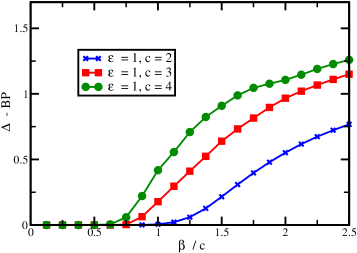
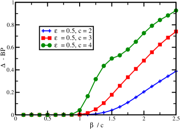
Whenever this deviation vanishes dynamic BP must have converged to a stationary state. Fig. 1 shows the results for various connectivity parameters in symmetric and partially symmetric networks. In high temperature we observe convergence towards a fixed point whereas in low temperature BP does not reach a stationary state. Roughly speaking, dynamic BP stops converging at a value βcr(c)subscript𝛽𝑐𝑟𝑐\beta_{cr}(c) which depends on average connectivity.
Refer to caption
Refer to caption
Figure 1: (Color online) Squared deviation of spin averages between successive update Δ(t)=1/Ni=1N(mi(t)mi(t1))2Δ𝑡1𝑁superscriptsubscript𝑖1𝑁superscriptsubscript𝑚𝑖𝑡subscript𝑚𝑖𝑡12\Delta(t)=1/N\sum_{i=1}^{N}\,(m_{i}(t)-m_{i}(t-1))^{2} at stationary limit for different values of average connectivity c𝑐c. Mean magnetizations are calculated by projected dynamic cavity method i.e Eq. 48. Left panel: partially asymmetric networks with ϵ=0.5italic-ϵ0.5\epsilon=0.5. Right panel : symmetric network ϵ=1italic-ϵ1\epsilon=1. The results are averaged over BP initial conditions (10 experiences). System size is 100010001000 and external fields are set to zero.

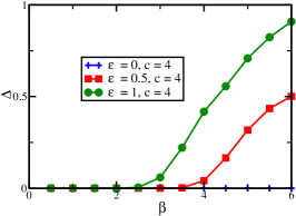
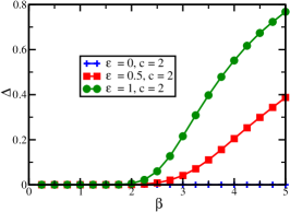
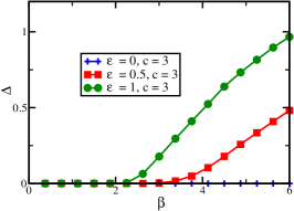
In Fig. 2 the convergence of dynamic BP is plotted to show the effect of asymmetry. In this case it is simply so that for very asymmetric graphs BP converges in a very wide region, presumably for arbitrarily large values of β𝛽\beta if the network grows large enough, and, in general, the more asymmetric the network, the better the convergence.
Refer to caption
Refer to caption
Refer to caption
Figure 2: (Color online) Effect of asymmetry (ϵ=0,0.5,1)italic-ϵ00.51(\epsilon=0,0.5,1) in squared deviation of spin averages between successive update Δ(t)=1/Ni=1N(mi(t)mi(t1))2Δ𝑡1𝑁superscriptsubscript𝑖1𝑁superscriptsubscript𝑚𝑖𝑡subscript𝑚𝑖𝑡12\Delta(t)=1/N\sum_{i=1}^{N}\,(m_{i}(t)-m_{i}(t-1))^{2}, obtained by projected dynamic BP Eq. 48, at stationary limit for average connectivity c=2𝑐2c=2 (left panel), c=3𝑐3c=3 (middle panel), c=4𝑐4c=4 (right panel). The results are averaged over BP initial conditions (10 experiences). System size is 100010001000 and external fields are set to zero.

V.2 Performance of dynamic BP

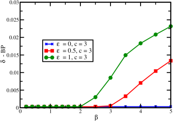
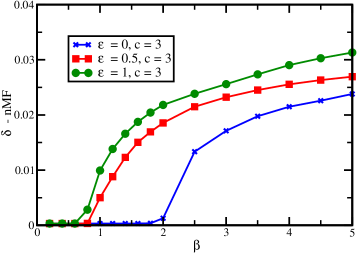
Fig. 3 shows a comparison between dynamic cavity method and dynamic mean field for total magnetization in spin glass systems with different asymmetric parameter. The results are obtained in present of small external fields θ=0.001𝜃0.001\theta=0.001. Dynamic cavity method shows a strong agreement with numerical simulations of type Glauber dynamics when it converges to a stationary state. The dynamic mean field method however starts to deviate from numerical simulations already in small β𝛽\beta indicating that it is less accurate compared to the dynamic cavity method.
Refer to caption
Refer to caption
Figure 3: (Color online) Mean square error δ(t)=1/Ni=1N(mipredicted(t)miempirical(t))2𝛿𝑡1𝑁superscriptsubscript𝑖1𝑁superscriptsuperscriptsubscript𝑚𝑖predicted𝑡superscriptsubscript𝑚𝑖empirical𝑡2\delta(t)=1/N\sum_{i=1}^{N}(m_{i}^{\rm predicted}(t)-m_{i}^{\rm empirical}(t))^{2} of the two approximation methods (dynamic mean field and dynamic cavity with respect to the empirical data (Glauber dynamics). Left panel: dynamic mean field (Eq. 21) for networks with different asymmetric parameter (ϵ=0,0.5,1)italic-ϵ00.51(\epsilon=0,0.5,1) and fixed average connectivity c=3𝑐3c=3. Right panel : the corresponding results obtained by the projected dynamic cavity method Eq. 48) For small β𝛽\beta, i.e. high temperature they are in agreement with numerical simulations. In low β𝛽\beta however, dynamic BP outperforms dynamic mean field.

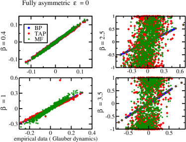
In order to observe the comparison in more detail, we show also the scatter plot of spin-by-spin magnetization in Fig.4. Dynamic cavity method predicts perfectly local magnetizations for fully asymmetric networks and agrees quite well with numerical simulations in high temperature for fully symmetric network whereas naive mean field and TAP start to deviate already at moderate temperatures.
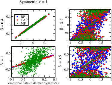
Refer to caption
Refer to caption
Figure 4: (Color online) Scatter plot of local magnetizations for dilute asymmetric networks for four different temperature β=0.4,1,2.5,3.5𝛽0.412.53.5\beta=0.4,1,2.5,3.5 and a fixed average connectivity c=3𝑐3c=3. Local magnetizations are obtained by dynamic mean field Eq. 21 (green), dynamic TAP Eq. 22 (red), and projected dynamic BP Eq. 48 (blue). Left panels show the scatter plots in fully asymmetric networks (ϵ=0italic-ϵ0\epsilon=0) where the projected dynamic BP provides exact results and right panels are scatter plots in fully symmetric networks (ϵ=1)italic-ϵ1(\epsilon=1). In high temperature, all three methods agree with numerical simulations. In low temperature BP starts to outperform naive mean field and TAP.

VI Conclusion

Message-passing methods have become an important topic on the border-line between equilibrium statistical physics and information theory. In the present paper we have studied an extension of message-passing to non-equilibrium Ising spin systems. In contrast to the equilibrium case, the cavity method is not immediately useful to describe the dynamics, even if the topology is suitable, because the messages depend on whole spin time histories. The time-factorization assumption, as discussed here and in Neri and Bollé (2009); Aurell and Mahmoudi (2011a, b), (or some other simplifying assumption) is necessary to reduce the complexity, but when so doing one is generally restricted to stationary states.

We have studied dynamic cavity in the time-factorized assumption for stationary states and outlined its convergence region in parameter strength (β𝛽\beta), connectivity (c𝑐c) and asymmetry (ϵitalic-ϵ\epsilon). By analogy with generally known facts about BP it can be argued that when dynamic cavity converges it should typically be a good approximation; the region of convergence is therefore a useful proxy for the accuracy. Expanding on first results presented in Aurell and Mahmoudi (2011a) we show that the convergence region in β𝛽\beta increases with the connectivity. We also find that the convergence region increases with asymmetry for several values of connectivity, and that it converges for any interaction strength for fully asymmetric networks (as expected). For networks of moderate size we have directly compared dynamic cavity and dynamic mean-field to direct simulation. For several values of asymmetry and connectivity we find that their convergence regions are very similar, if not identical, but when both methods converge, then dynamic cavity is considerably more accurate, except in the low β𝛽\beta limit where their performance is about the same. We have hence showed that dynamic cavity can be useful new approximation to the dynamics of non-equilibrium spin systems – and any system which can be fruitfully modeled by such methods.

On the analytical side we have discussed the special status of fully asymmetric models, for which the cavity approach is in some sense exact. We have also re-derived the “dynamic TAP” equation of Hertz and Roudi Hertz and Roudi (2011); Roudi and Hertz (2011) using a straight-forward approach borrowed from Kappen and Spanjers’ treatment of the stationary state Kappen and Spanjers (2000) clarifying that this approach is based on minimizing the distance, in the sense of Information Geometry, to the sub-family of independent (but time-changing) models. Whether such a perturbative argument can be extended to small deviations from e.g. fully asymmetric models remains to be seen.

Acknowledgment

We thank Marc Mézard for important remarks, and Mikko Alava, Yoshiyuki Kabashima, Pekka Orponen and Toshiyuki Tanaka for discussions. The work was supported by the Academy of Finland as part of its Finland Distinguished Professor program, project 129024/Aurell.

Appendix A The Information Geometry calculation to second order

The following calculations are completely parallel to those in Appendix 1 of Kappen and Spanjers (2000) and start from

mi(t)θj(s)|indevaluated-atsubscript𝑚𝑖𝑡subscript𝜃𝑗𝑠ind\displaystyle\frac{\partial m_{i}(t)}{\partial\theta_{j}(s)}|_{\hbox{ind}} =\displaystyle= δs,tδij(1mi2(t))subscript𝛿𝑠𝑡subscript𝛿𝑖𝑗1superscriptsubscript𝑚𝑖2𝑡\displaystyle\delta_{s,t}\delta_{ij}(1-m_{i}^{2}(t)) (50)
mi(t)Jjk|indevaluated-atsubscript𝑚𝑖𝑡subscript𝐽𝑗𝑘ind\displaystyle\frac{\partial m_{i}(t)}{\partial J_{jk}}|_{\hbox{ind}} =\displaystyle= δik(1mi2(t))mj(t1)subscript𝛿𝑖𝑘1superscriptsubscript𝑚𝑖2𝑡subscript𝑚𝑗𝑡1\displaystyle\delta_{ik}(1-m_{i}^{2}(t))m_{j}(t-1) (51)
2mi(t)θj(s)θk(s)|indevaluated-atsuperscript2subscript𝑚𝑖𝑡subscript𝜃𝑗𝑠subscript𝜃𝑘superscript𝑠ind\displaystyle\frac{\partial^{2}m_{i}(t)}{\partial\theta_{j}(s)\partial\theta_{k}(s^{\prime})}|_{\hbox{ind}} =\displaystyle= 2mi(t)(1mi2(t))δijδikδs,tδs,t2subscript𝑚𝑖𝑡1subscriptsuperscript𝑚2𝑖𝑡subscript𝛿𝑖𝑗subscript𝛿𝑖𝑘subscript𝛿𝑠𝑡subscript𝛿superscript𝑠𝑡\displaystyle-2m_{i}(t)(1-m^{2}_{i}(t))\delta_{ij}\delta_{ik}\delta_{s,t}\delta_{s^{\prime},t} (52)
2mi(t)Jjkθl(s)|indevaluated-atsuperscript2subscript𝑚𝑖𝑡subscript𝐽𝑗𝑘subscript𝜃𝑙𝑠ind\displaystyle\frac{\partial^{2}m_{i}(t)}{\partial J_{jk}\partial\theta_{l}(s)}|_{\hbox{ind}} =\displaystyle= 2mi(t)(1mi2(t))mj(t1)δikδilδs,t2subscript𝑚𝑖𝑡1subscriptsuperscript𝑚2𝑖𝑡subscript𝑚𝑗𝑡1subscript𝛿𝑖𝑘subscript𝛿𝑖𝑙subscript𝛿𝑠𝑡\displaystyle-2m_{i}(t)(1-m^{2}_{i}(t))m_{j}(t-1)\delta_{ik}\delta_{il}\delta_{s,t} (53)
+(1mi2(t))(1mj2(t1))δikδklδs,t11subscriptsuperscript𝑚2𝑖𝑡1superscriptsubscript𝑚𝑗2𝑡1subscript𝛿𝑖𝑘subscript𝛿𝑘𝑙subscript𝛿𝑠𝑡1\displaystyle+(1-m^{2}_{i}(t))(1-m_{j}^{2}(t-1))\delta_{ik}\delta_{kl}\delta_{s,t-1}
2mi(t)JjkJlm|indevaluated-atsuperscript2subscript𝑚𝑖𝑡subscript𝐽𝑗𝑘subscript𝐽𝑙𝑚ind\displaystyle\frac{\partial^{2}m_{i}(t)}{\partial J_{jk}\partial J_{lm}}|_{\hbox{ind}} =\displaystyle= δik(1mi2(t))(1mj2(t1))δlkml(t2)+(jk)(lm)subscript𝛿𝑖𝑘1superscriptsubscript𝑚𝑖2𝑡1superscriptsubscript𝑚𝑗2𝑡1subscript𝛿𝑙𝑘subscript𝑚𝑙𝑡2𝑗𝑘𝑙𝑚\displaystyle\delta_{ik}(1-m_{i}^{2}(t))(1-m_{j}^{2}(t-1))\delta_{lk}m_{l}(t-2)+(jk)\leftrightarrow(lm) (54)
2mi(t)δik(1mi2(t))δim(mk(t1)mm(t1)+δkm(1mk2(t1)))2subscript𝑚𝑖𝑡subscript𝛿𝑖𝑘1superscriptsubscript𝑚𝑖2𝑡subscript𝛿𝑖𝑚subscript𝑚𝑘𝑡1subscript𝑚𝑚𝑡1subscript𝛿𝑘𝑚1superscriptsubscript𝑚𝑘2𝑡1\displaystyle-2m_{i}(t)\delta_{ik}(1-m_{i}^{2}(t))\delta_{im}\left(m_{k}(t-1)m_{m}(t-1)+\delta_{km}(1-m_{k}^{2}(t-1))\right)

To first order in ϵitalic-ϵ\epsilon (26) hence gives

s,jδs,tδij(1mi2(t))Δj(1)(s)+jkδij(1mi2(t))mk(t1)Jjk=0subscript𝑠𝑗subscript𝛿𝑠𝑡subscript𝛿𝑖𝑗1superscriptsubscript𝑚𝑖2𝑡subscriptsuperscriptΔ1𝑗𝑠subscript𝑗𝑘subscript𝛿𝑖𝑗1superscriptsubscript𝑚𝑖2𝑡subscript𝑚𝑘𝑡1subscript𝐽𝑗𝑘0\sum_{s,j}\delta_{s,t}\delta_{ij}(1-m_{i}^{2}(t))\Delta^{(1)}_{j}(s)+\sum_{jk}\delta_{ij}(1-m_{i}^{2}(t))m_{k}(t-1)J_{jk}=0 (55)

which is simply

Ai(1)(t)Δi(1)(t)+jJjimj(t1)=0subscriptsuperscript𝐴1𝑖𝑡subscriptsuperscriptΔ1𝑖𝑡subscript𝑗subscript𝐽𝑗𝑖subscript𝑚𝑗𝑡10A^{(1)}_{i}(t)\equiv\Delta^{(1)}_{i}(t)+\sum_{j}J_{ji}m_{j}(t-1)=0 (56)

This is the same as ”dynamic naive mean field”

tanh1(mi(t))=θi(t)+kJkimk(t1)+𝒪(ϵ2)superscript1subscript𝑚𝑖𝑡subscript𝜃𝑖𝑡subscript𝑘subscript𝐽𝑘𝑖subscript𝑚𝑘𝑡1𝒪superscriptitalic-ϵ2\tanh^{-1}(m_{i}(t))=\theta_{i}(t)+\sum_{k}J_{ki}m_{k}(t-1)+{\cal O}(\epsilon^{2}) (57)

The terms arising from second order derivatives and first order increments can be grouped together as

(1mi2(t))(mi(t)(Ai(1))2(t)j(1mj2(t1))JjiAj(1)(t1)mi(t)kJki2(1mk2(t1)))1superscriptsubscript𝑚𝑖2𝑡subscript𝑚𝑖𝑡superscriptsubscriptsuperscript𝐴1𝑖2𝑡subscript𝑗1superscriptsubscript𝑚𝑗2𝑡1subscript𝐽𝑗𝑖subscriptsuperscript𝐴1𝑗𝑡1subscript𝑚𝑖𝑡subscript𝑘superscriptsubscript𝐽𝑘𝑖21superscriptsubscript𝑚𝑘2𝑡1(1-m_{i}^{2}(t))\left(-m_{i}(t)(A^{(1)}_{i})^{2}(t)-\sum_{j}(1-m_{j}^{2}(t-1))J_{ji}A^{(1)}_{j}(t-1)-m_{i}(t)\sum_{k}J_{ki}^{2}(1-m_{k}^{2}(t-1))\right) (58)

which together with the first order conditions (56) and the term from the first order derivative and second order increment (1mi2(t))Δi(2)(t)1superscriptsubscript𝑚𝑖2𝑡subscriptsuperscriptΔ2𝑖𝑡(1-m_{i}^{2}(t))\Delta^{(2)}_{i}(t) gives

Δi(2)(t)=mi(t)kJki2(1mk2(t1))subscriptsuperscriptΔ2𝑖𝑡subscript𝑚𝑖𝑡subscript𝑘superscriptsubscript𝐽𝑘𝑖21superscriptsubscript𝑚𝑘2𝑡1\Delta^{(2)}_{i}(t)=m_{i}(t)\sum_{k}J_{ki}^{2}(1-m_{k}^{2}(t-1)) (59)

This is the same as “dynamic TAP”, compare (22) above

tanh1(mi(t))=θi(t)+kJkimk(t1)mi(t)kJki2mk2(t1)+𝒪(ϵ3)superscript1subscript𝑚𝑖𝑡subscript𝜃𝑖𝑡subscript𝑘subscript𝐽𝑘𝑖subscript𝑚𝑘𝑡1subscript𝑚𝑖𝑡subscript𝑘superscriptsubscript𝐽𝑘𝑖2superscriptsubscript𝑚𝑘2𝑡1𝒪superscriptitalic-ϵ3\tanh^{-1}(m_{i}(t))=\theta_{i}(t)+\sum_{k}J_{ki}m_{k}(t-1)-m_{i}(t)\sum_{k}J_{ki}^{2}m_{k}^{2}(t-1)+{\cal O}(\epsilon^{3}) (60)

Appendix B The Information Geometry calculation to third order

Third order contributions consist partly of terms involving lower than third order derivatives and higher than first order increments. The calculation of these use the same elements as above and are

j,smi(t)θj(s)|indΔj(3)(s)evaluated-atsubscript𝑗𝑠subscript𝑚𝑖𝑡subscript𝜃𝑗𝑠indsubscriptsuperscriptΔ3𝑗𝑠\displaystyle\sum_{j,s}\frac{\partial m_{i}(t)}{\partial\theta_{j}(s)}|_{\hbox{ind}}\Delta^{(3)}_{j}(s) =\displaystyle= (1mi2(t))Δi(3)(t)1superscriptsubscript𝑚𝑖2𝑡subscriptsuperscriptΔ3𝑖𝑡\displaystyle(1-m_{i}^{2}(t))\Delta^{(3)}_{i}(t) (61)
j,s,k,s2mi(t)θj(s)θk(s)|indΔj(2)(s)Δk(1)(s)evaluated-atsubscript𝑗𝑠𝑘superscript𝑠superscript2subscript𝑚𝑖𝑡subscript𝜃𝑗𝑠subscript𝜃𝑘superscript𝑠indsubscriptsuperscriptΔ2𝑗𝑠subscriptsuperscriptΔ1𝑘superscript𝑠\displaystyle\sum_{j,s,k,s^{\prime}}\frac{\partial^{2}m_{i}(t)}{\partial\theta_{j}(s)\partial\theta_{k}(s^{\prime})}|_{\hbox{ind}}\Delta^{(2)}_{j}(s)\Delta^{(1)}_{k}(s^{\prime}) =\displaystyle= 2mi(t)(1mi2(t))Δi(2)(t)Δi(1)(t)2subscript𝑚𝑖𝑡1subscriptsuperscript𝑚2𝑖𝑡subscriptsuperscriptΔ2𝑖𝑡subscriptsuperscriptΔ1𝑖𝑡\displaystyle-2m_{i}(t)(1-m^{2}_{i}(t))\Delta^{(2)}_{i}(t)\Delta^{(1)}_{i}(t) (62)
j,k,l,s2mi(t)Jjkθl(s)|indJjkΔl(2)(s)evaluated-atsubscript𝑗𝑘𝑙𝑠superscript2subscript𝑚𝑖𝑡subscript𝐽𝑗𝑘subscript𝜃𝑙𝑠indsubscript𝐽𝑗𝑘subscriptsuperscriptΔ2𝑙𝑠\displaystyle\sum_{j,k,l,s}\frac{\partial^{2}m_{i}(t)}{\partial J_{jk}\partial\theta_{l}(s)}|_{\hbox{ind}}J_{jk}\Delta^{(2)}_{l}(s) =\displaystyle= 2mi(t)(1mi2(t))jmj(t1)JjiΔi(2)(t)2subscript𝑚𝑖𝑡1subscriptsuperscript𝑚2𝑖𝑡subscript𝑗subscript𝑚𝑗𝑡1subscript𝐽𝑗𝑖subscriptsuperscriptΔ2𝑖𝑡\displaystyle-2m_{i}(t)(1-m^{2}_{i}(t))\sum_{j}m_{j}(t-1)J_{ji}\Delta^{(2)}_{i}(t) (63)
+(1mi2(t))k(1mk2(t1))JkiΔk(2)(t1)1subscriptsuperscript𝑚2𝑖𝑡subscript𝑘1superscriptsubscript𝑚𝑘2𝑡1subscript𝐽𝑘𝑖subscriptsuperscriptΔ2𝑘𝑡1\displaystyle+(1-m^{2}_{i}(t))\sum_{k}(1-m_{k}^{2}(t-1))J_{ki}\Delta^{(2)}_{k}(t-1)

where two terms can be combined to

2mi(t)(1mi2(t))Δi(2)(t)(Δi(1)(t)+kJkimk(t1))=0.2subscript𝑚𝑖𝑡1superscriptsubscript𝑚𝑖2𝑡subscriptsuperscriptΔ2𝑖𝑡subscriptsuperscriptΔ1𝑖𝑡subscript𝑘subscript𝐽𝑘𝑖subscript𝑚𝑘𝑡10-2m_{i}(t)(1-m_{i}^{2}(t))\Delta^{(2)}_{i}(t)\left(\Delta^{(1)}_{i}(t)+\sum_{k}J_{ki}m_{k}(t-1)\right)=0. (64)

The remainder is

(1mi2(t))(Δi(3)(t)+k(1mk2(t1))JkiΔk(2)(t1))(lower order terms)1superscriptsubscript𝑚𝑖2𝑡subscriptsuperscriptΔ3𝑖𝑡subscript𝑘1superscriptsubscript𝑚𝑘2𝑡1subscript𝐽𝑘𝑖subscriptsuperscriptΔ2𝑘𝑡1(lower order terms)(1-m_{i}^{2}(t))\left(\Delta^{(3)}_{i}(t)+\sum_{k}(1-m_{k}^{2}(t-1))J_{ki}\Delta^{(2)}_{k}(t-1)\right)\qquad\hbox{(lower order terms)} (65)

To proceed with the terms from third order derivatives and first order increments it is useful to introduce the streamlined notation

mi=mi(t)mi=mi(t1)mi′′=mi(t2)etc.formulae-sequencesubscript𝑚𝑖subscript𝑚𝑖𝑡formulae-sequencesuperscriptsubscript𝑚𝑖subscript𝑚𝑖𝑡1superscriptsubscript𝑚𝑖′′subscript𝑚𝑖𝑡2etc.m_{i}=m_{i}(t)\qquad m_{i}^{\prime}=m_{i}(t-1)\qquad m_{i}^{\prime\prime}=m_{i}(t-2)\qquad\hbox{etc.} (66)

and similar for all other quantities. It is also useful to note that though the derivatives act on the complete expression involving both probability density P𝑃P and the tanh\tanh they partially obey a chain rule when taken to act on the magnetizations alone:

  • a derivative with respect to an external field θj(s)subscript𝜃𝑗𝑠\theta_{j}(s) functions as an ordinary derivative and obeys a chain rule;

  • a derivative with respect to an interaction coefficient Jklsubscript𝐽𝑘𝑙J_{kl} acting on a once or more than once primed quantity, such as misuperscriptsubscript𝑚𝑖m_{i}^{\prime} and mi′′superscriptsubscript𝑚𝑖′′m_{i}^{\prime\prime}, functions as an ordinary derivative and obeys the chain rule;

  • a derivative with respect to an interaction coefficient Jklsubscript𝐽𝑘𝑙J_{kl} acting on an unprimed quantity such as misubscript𝑚𝑖m_{i} must be treated apart, since this derivative will include a term taken on the tanh\tanh, which in turn will give a higher order correlation.

These rules allow us to continue from what has already been computed and write

miθj(s)|indevaluated-atsubscript𝑚𝑖subscript𝜃𝑗𝑠ind\displaystyle\frac{\partial m_{i}}{\partial\theta_{j}(s)}|_{\hbox{ind}} =\displaystyle= (1mi2)δijδst1superscriptsubscript𝑚𝑖2subscript𝛿𝑖𝑗subscript𝛿𝑠𝑡\displaystyle(1-m_{i}^{2})\delta_{ij}\delta_{st}
2miθj(s)θk(s)|indevaluated-atsuperscript2subscript𝑚𝑖subscript𝜃𝑗𝑠subscript𝜃𝑘superscript𝑠ind\displaystyle\frac{\partial^{2}m_{i}}{\partial\theta_{j}(s)\partial\theta_{k}(s^{\prime})}|_{\hbox{ind}} =\displaystyle= 2mi(1mi2)δijδstδikδst2subscript𝑚𝑖1superscriptsubscript𝑚𝑖2subscript𝛿𝑖𝑗subscript𝛿𝑠𝑡subscript𝛿𝑖𝑘subscript𝛿superscript𝑠𝑡\displaystyle-2m_{i}(1-m_{i}^{2})\delta_{ij}\delta_{st}\delta_{ik}\delta_{s^{\prime}t}
3miθj(s)θk(s)θl(s′′)|indevaluated-atsuperscript3subscript𝑚𝑖subscript𝜃𝑗𝑠subscript𝜃𝑘superscript𝑠subscript𝜃𝑙superscript𝑠′′ind\displaystyle\frac{\partial^{3}m_{i}}{\partial\theta_{j}(s)\partial\theta_{k}(s^{\prime})\partial\theta_{l}(s^{\prime\prime})}|_{\hbox{ind}} =\displaystyle= 2(1mi2)(3mi21)δijδstδikδstδilδs′′t21superscriptsubscript𝑚𝑖23superscriptsubscript𝑚𝑖21subscript𝛿𝑖𝑗subscript𝛿𝑠𝑡subscript𝛿𝑖𝑘subscript𝛿superscript𝑠𝑡subscript𝛿𝑖𝑙subscript𝛿superscript𝑠′′𝑡\displaystyle 2(1-m_{i}^{2})(3m_{i}^{2}-1)\delta_{ij}\delta_{st}\delta_{ik}\delta_{s^{\prime}t}\delta_{il}\delta_{s^{\prime\prime}t}
\displaystyle\vdots

For the mixed terms we have similarly

miJjk|indevaluated-atsubscript𝑚𝑖subscript𝐽𝑗𝑘ind\displaystyle\frac{\partial m_{i}}{\partial J_{jk}}|_{\hbox{ind}} =\displaystyle= (1mi2)δikmj1superscriptsubscript𝑚𝑖2subscript𝛿𝑖𝑘subscriptsuperscript𝑚𝑗\displaystyle(1-m_{i}^{2})\delta_{ik}m^{\prime}_{j}
2miJjkθl(s)|indevaluated-atsuperscript2subscript𝑚𝑖subscript𝐽𝑗𝑘subscript𝜃𝑙𝑠ind\displaystyle\frac{\partial^{2}m_{i}}{\partial J_{jk}\partial\theta_{l}(s)\partial}|_{\hbox{ind}} =\displaystyle= 2mi(1mi2)δilδs,tδikmj+(1mi2)δik(1(mj)2)δjlδs,t12subscript𝑚𝑖1superscriptsubscript𝑚𝑖2subscript𝛿𝑖𝑙subscript𝛿𝑠𝑡subscript𝛿𝑖𝑘subscriptsuperscript𝑚𝑗1superscriptsubscript𝑚𝑖2subscript𝛿𝑖𝑘1superscriptsubscriptsuperscript𝑚𝑗2subscript𝛿𝑗𝑙subscript𝛿𝑠𝑡1\displaystyle-2m_{i}(1-m_{i}^{2})\delta_{il}\delta_{s,t}\delta_{ik}m^{\prime}_{j}+(1-m_{i}^{2})\delta_{ik}(1-(m^{\prime}_{j})^{2})\delta_{jl}\delta_{s,t-1}
3miJjkθl(s)θl(s)|indevaluated-atsuperscript3subscript𝑚𝑖subscript𝐽𝑗𝑘subscript𝜃𝑙𝑠subscript𝜃superscript𝑙superscript𝑠ind\displaystyle\frac{\partial^{3}m_{i}}{\partial J_{jk}\partial\theta_{l}(s)\partial\theta_{l^{\prime}}(s^{\prime})}|_{\hbox{ind}} =\displaystyle= 2(1mi2)(3mi21)δilδs,tδilδs,tδikmj21superscriptsubscript𝑚𝑖23superscriptsubscript𝑚𝑖21subscript𝛿𝑖superscript𝑙subscript𝛿superscript𝑠𝑡subscript𝛿𝑖𝑙subscript𝛿𝑠𝑡subscript𝛿𝑖𝑘subscriptsuperscript𝑚𝑗\displaystyle 2(1-m_{i}^{2})(3m_{i}^{2}-1)\delta_{il^{\prime}}\delta_{s^{\prime},t}\delta_{il}\delta_{s,t}\delta_{ik}m^{\prime}_{j}
\displaystyle- 2mi(1mi2)δilδs,tδik(1(mj)2)δljδs,t12subscript𝑚𝑖1superscriptsubscript𝑚𝑖2subscript𝛿𝑖𝑙subscript𝛿𝑠𝑡subscript𝛿𝑖𝑘1superscriptsubscriptsuperscript𝑚𝑗2subscript𝛿superscript𝑙𝑗subscript𝛿superscript𝑠𝑡1\displaystyle 2m_{i}(1-m_{i}^{2})\delta_{il}\delta_{s,t}\delta_{ik}(1-(m^{\prime}_{j})^{2})\delta_{l^{\prime}j}\delta_{s^{\prime},t-1}
\displaystyle- 2mi(1mi2)δilδs,tδik(1(mj)2)δjlδs,t12subscript𝑚𝑖1superscriptsubscript𝑚𝑖2subscript𝛿𝑖superscript𝑙subscript𝛿superscript𝑠𝑡subscript𝛿𝑖𝑘1superscriptsubscriptsuperscript𝑚𝑗2subscript𝛿𝑗𝑙subscript𝛿𝑠𝑡1\displaystyle 2m_{i}(1-m_{i}^{2})\delta_{il^{\prime}}\delta_{s^{\prime},t}\delta_{ik}(1-(m^{\prime}_{j})^{2})\delta_{jl}\delta_{s,t-1}
+\displaystyle+ (1mi2)δik(2mj)(1(mj)2)δjlδs,t1δjlδs,t11superscriptsubscript𝑚𝑖2subscript𝛿𝑖𝑘2subscriptsuperscript𝑚𝑗1superscriptsubscriptsuperscript𝑚𝑗2subscript𝛿𝑗𝑙subscript𝛿𝑠𝑡1subscript𝛿𝑗superscript𝑙subscript𝛿superscript𝑠𝑡1\displaystyle(1-m_{i}^{2})\delta_{ik}(-2m^{\prime}_{j})(1-(m^{\prime}_{j})^{2})\delta_{jl}\delta_{s,t-1}\delta_{jl^{\prime}}\delta_{s^{\prime},t-1}
\displaystyle\vdots

and

2miJjkJlm|indevaluated-atsuperscript2subscript𝑚𝑖subscript𝐽𝑗𝑘subscript𝐽𝑙𝑚ind\displaystyle\frac{\partial^{2}m_{i}}{\partial J_{jk}\partial J_{lm}}|_{\hbox{ind}} =\displaystyle= δik(1mi2)(1(mj)2)δlkml′′+(jk)(lm)subscript𝛿𝑖𝑘1superscriptsubscript𝑚𝑖21superscriptsubscriptsuperscript𝑚𝑗2subscript𝛿𝑙𝑘subscriptsuperscript𝑚′′𝑙𝑗𝑘𝑙𝑚\displaystyle\delta_{ik}(1-m_{i}^{2})(1-(m^{\prime}_{j})^{2})\delta_{lk}m^{{}^{\prime\prime}}_{l}+(jk)\leftrightarrow(lm)
2mi(1mi2)δikδim(mkmm+χkm))\displaystyle-2m_{i}(1-m_{i}^{2})\delta_{ik}\delta_{im}\left(m^{\prime}_{k}m^{\prime}_{m}+\chi^{\prime}_{km})\right)
3miJjkJlmθn(s)|indevaluated-atsuperscript3subscript𝑚𝑖subscript𝐽𝑗𝑘subscript𝐽𝑙𝑚subscript𝜃𝑛𝑠ind\displaystyle\frac{\partial^{3}m_{i}}{\partial J_{jk}\partial J_{lm}\partial\theta_{n}(s)}|_{\hbox{ind}} =\displaystyle= δik(2mi(1mi2)δinδs,t(1(mj)2)δlkml′′\displaystyle\delta_{ik}(-2m_{i}(1-m_{i}^{2})\delta_{in}\delta_{s,t}(1-(m^{\prime}_{j})^{2})\delta_{lk}m^{{}^{\prime\prime}}_{l}
+δik(1mi2)(2mj(1(mj)2)δjnδs,t1δlkml′′\displaystyle\quad+\delta_{ik}(1-m_{i}^{2})(-2m^{\prime}_{j}(1-(m^{\prime}_{j})^{2})\delta_{jn}\delta_{s,t-1}\delta_{lk}m^{{}^{\prime\prime}}_{l}
+δik(1mi2)(1(mj)2)δlk(1(ml′′)2)δlnδs,t2subscript𝛿𝑖𝑘1superscriptsubscript𝑚𝑖21superscriptsubscriptsuperscript𝑚𝑗2subscript𝛿𝑙𝑘1superscriptsubscriptsuperscript𝑚′′𝑙2subscript𝛿𝑙𝑛subscript𝛿𝑠𝑡2\displaystyle\quad\quad+\delta_{ik}(1-m_{i}^{2})(1-(m^{\prime}_{j})^{2})\delta_{lk}(1-(m^{{}^{\prime\prime}}_{l})^{2})\delta_{ln}\delta_{s,t-2}
+\displaystyle+ (jk)(lm)𝑗𝑘𝑙𝑚\displaystyle(jk)\leftrightarrow(lm)
+\displaystyle+ 2(1mi2)(3mi²1)δinδs,tδikδim<σk(t1)σm(t1)>21superscriptsubscript𝑚𝑖23subscript𝑚𝑖²1subscript𝛿𝑖𝑛subscript𝛿𝑠𝑡subscript𝛿𝑖𝑘subscript𝛿𝑖𝑚expectationsubscript𝜎𝑘𝑡1subscript𝜎𝑚𝑡1\displaystyle 2(1-m_{i}^{2})(3m_{i}\texttwosuperior-1)\delta_{in}\delta_{s,t}\delta_{ik}\delta_{im}<\sigma_{k}(t-1)\sigma_{m}(t-1)>
2mi(1mi2)δikδim(1(mk)2)δknδs,t1mm2subscript𝑚𝑖1superscriptsubscript𝑚𝑖2subscript𝛿𝑖𝑘subscript𝛿𝑖𝑚1superscriptsubscriptsuperscript𝑚𝑘2subscript𝛿𝑘𝑛subscript𝛿𝑠𝑡1subscriptsuperscript𝑚𝑚\displaystyle\quad-2m_{i}(1-m_{i}^{2})\delta_{ik}\delta_{im}(1-(m^{\prime}_{k})^{2})\delta_{kn}\delta_{s,t-1}m^{\prime}_{m}
2mi(1mi2)δikδimmk(1(mm)2)δmnδs,t12subscript𝑚𝑖1superscriptsubscript𝑚𝑖2subscript𝛿𝑖𝑘subscript𝛿𝑖𝑚subscriptsuperscript𝑚𝑘1superscriptsubscriptsuperscript𝑚𝑚2subscript𝛿𝑚𝑛subscript𝛿𝑠𝑡1\displaystyle\quad\quad-2m_{i}(1-m_{i}^{2})\delta_{ik}\delta_{im}m^{\prime}_{k}(1-(m^{\prime}_{m})^{2})\delta_{mn}\delta_{s,t-1}
2mi(1mi2)δikδimχkmθn(s)2subscript𝑚𝑖1superscriptsubscript𝑚𝑖2subscript𝛿𝑖𝑘subscript𝛿𝑖𝑚subscriptsuperscript𝜒𝑘𝑚subscript𝜃𝑛𝑠\displaystyle\quad\quad\quad-2m_{i}(1-m_{i}^{2})\delta_{ik}\delta_{im}\frac{\partial\chi^{\prime}_{km}}{\partial\theta_{n}(s)}
\displaystyle\vdots

where we use the correlation function χkm=<σk(t)σm(t)>mkmmsubscript𝜒𝑘𝑚expectationsubscript𝜎𝑘𝑡subscript𝜎𝑚𝑡subscript𝑚𝑘subscript𝑚𝑚\chi_{km}=<\sigma_{k}(t)\sigma_{m}(t)>-m_{k}m_{m}. Its partial derivative with respect to an external field is always zero, and the last term in above therefore vanishes. The more cumbersome term is three derivatives with respect to interaction coefficients, which we can start from

3mipqJjkJlm|ind=Jpq[σ2P(σ)JjkJlmtanh()+σP(σ)Jjk(1tanh2())δimσl(t1)+(jk)(lm)σP(σ)(2tanh())(1tanh2())δimσl(t1)δikσj(t1)]evaluated-atsuperscript3subscript𝑚𝑖subscript𝑝𝑞subscript𝐽𝑗𝑘subscript𝐽𝑙𝑚indsubscript𝐽𝑝𝑞delimited-[]limit-fromsubscript𝜎superscript2𝑃𝜎subscript𝐽𝑗𝑘subscript𝐽𝑙𝑚subscript𝜎𝑃𝜎subscript𝐽𝑗𝑘1superscript2subscript𝛿𝑖𝑚subscript𝜎𝑙𝑡1𝑗𝑘𝑙𝑚subscript𝜎𝑃𝜎21superscript2subscript𝛿𝑖𝑚subscript𝜎𝑙𝑡1subscript𝛿𝑖𝑘subscript𝜎𝑗𝑡1\frac{\partial^{3}m_{i}}{\partial_{pq}\partial J_{jk}\partial J_{lm}}|_{\hbox{ind}}=\frac{\partial}{\partial J_{pq}}\left[\begin{array}[]{l}\sum_{\sigma}\frac{\partial^{2}P(\sigma)}{\partial J_{jk}\partial J_{lm}}\tanh(\cdot)+\\ \sum_{\sigma}\frac{\partial P(\sigma)}{\partial J_{jk}}(1-\tanh^{2}(\cdot))\delta_{im}\sigma_{l}(t-1)\\ \qquad+(jk)\leftrightarrow(lm)\\ \sum_{\sigma}P(\sigma)(-2\tanh(\cdot))(1-\tanh^{2}(\cdot))\delta_{im}\sigma_{l}(t-1)\delta_{ik}\sigma_{j}(t-1)\\ \end{array}\right] (67)

Applying Jpqsubscript𝐽𝑝𝑞\partial J_{pq} gives (at least conceptually) eight terms. The term from acting on 2P(σ)JjkJlmsuperscript2𝑃𝜎subscript𝐽𝑗𝑘subscript𝐽𝑙𝑚\frac{\partial^{2}P(\sigma)}{\partial J_{jk}\partial J_{lm}} vanishes. The term from acting on tanh()\tanh(\cdot) in the first line gives a second derivative with respect to interaction coefficients of a magnetization. The terms from the second and the third line give combinations involving either second derivatives of a magnetization, or first derivatives of a correlation function. The terms from the last line are a third order correlation function and further first deritives of second order correlation functions.

Taking all together we can sum the contributions to

Third order =\displaystyle= 162(1mi2)(3mi21)(Ai(1)(t))31621superscriptsubscript𝑚𝑖23superscriptsubscript𝑚𝑖21superscriptsubscriptsuperscript𝐴1𝑖𝑡3\displaystyle\frac{1}{6}2(1-m_{i}^{2})(3m_{i}^{2}-1)(A^{(1)}_{i}(t))^{3} (68)
+\displaystyle+ 2mi(1mi2)Δi(1)(t)l(1(ml)2)JliAl(1)(t1)2subscript𝑚𝑖1superscriptsubscript𝑚𝑖2subscriptsuperscriptΔ1𝑖𝑡subscript𝑙1superscriptsubscriptsuperscript𝑚𝑙2subscript𝐽𝑙𝑖subscriptsuperscript𝐴1𝑙𝑡1\displaystyle 2m_{i}(1-m_{i}^{2})\Delta^{(1)}_{i}(t)\sum_{l}(1-(m^{\prime}_{l})^{2})J_{li}A^{(1)}_{l}(t-1)
\displaystyle- (1mi2)lJli(Al(1)(t))21superscriptsubscript𝑚𝑖2subscript𝑙subscript𝐽𝑙𝑖superscriptsubscriptsuperscript𝐴1𝑙𝑡2\displaystyle(1-m_{i}^{2})\sum_{l}J_{li}(A^{(1)}_{l}(t))^{2}
+\displaystyle+ 122(1mi2)(3mi21)Ai(1)(t)lmJilJimχlm1221superscriptsubscript𝑚𝑖23superscriptsubscript𝑚𝑖21subscriptsuperscript𝐴1𝑖𝑡subscript𝑙𝑚subscript𝐽𝑖𝑙subscript𝐽𝑖𝑚subscript𝜒𝑙𝑚\displaystyle\frac{1}{2}2(1-m_{i}^{2})(3m_{i}^{2}-1)A^{(1)}_{i}(t)\sum_{lm}J_{il}J_{im}\chi_{lm}
\displaystyle- 2mi(1mi2)lnJli(1(ml)2)Al(1)(t1)Jnimn2subscript𝑚𝑖1superscriptsubscript𝑚𝑖2subscript𝑙𝑛subscript𝐽𝑙𝑖1superscriptsubscriptsuperscript𝑚𝑙2subscriptsuperscript𝐴1𝑙𝑡1subscript𝐽𝑛𝑖subscriptsuperscript𝑚𝑛\displaystyle 2m_{i}(1-m_{i}^{2})\sum_{ln}J_{li}(1-(m^{\prime}_{l})^{2})A^{(1)}_{l}(t-1)J_{ni}m^{\prime}_{n}
+\displaystyle+ (1mi2)mlJmiJlm(1(mm)2)(1(ml′′)2)Al(1)(t2)+(m)(l)1superscriptsubscript𝑚𝑖2subscript𝑚𝑙subscript𝐽𝑚𝑖subscript𝐽𝑙𝑚1superscriptsubscriptsuperscript𝑚𝑚21superscriptsubscriptsuperscript𝑚′′𝑙2subscriptsuperscript𝐴1𝑙𝑡2𝑚𝑙\displaystyle(1-m_{i}^{2})\sum_{ml}J_{mi}J_{lm}(1-(m^{\prime}_{m})^{2})(1-(m^{{}^{\prime\prime}}_{l})^{2})A^{(1)}_{l}(t-2)+(m)\leftrightarrow(l)
\displaystyle- mi(1mi2)ln,jsJliJni(χln(t1)θj(s))Δj(1)(s)subscript𝑚𝑖1superscriptsubscript𝑚𝑖2subscript𝑙𝑛𝑗𝑠subscript𝐽𝑙𝑖subscript𝐽𝑛𝑖subscript𝜒𝑙𝑛𝑡1subscript𝜃𝑗𝑠subscriptsuperscriptΔ1𝑗𝑠\displaystyle m_{i}(1-m_{i}^{2})\sum_{ln,js}J_{li}J_{ni}\left(\frac{\partial\chi_{ln}(t-1)}{\partial\theta_{j}(s)}\right)\Delta^{(1)}_{j}(s)
\displaystyle- 13mi(1mi2)ln,jsJliJni(χln(t1)Jpq)Jpq+circ. perm.13subscript𝑚𝑖1superscriptsubscript𝑚𝑖2subscript𝑙𝑛𝑗𝑠subscript𝐽𝑙𝑖subscript𝐽𝑛𝑖subscript𝜒𝑙𝑛𝑡1subscript𝐽𝑝𝑞subscript𝐽𝑝𝑞circ. perm.\displaystyle\frac{1}{3}m_{i}(1-m_{i}^{2})\sum_{ln,js}J_{li}J_{ni}\left(\frac{\partial\chi_{ln}(t-1)}{\partial J_{pq}}\right)J_{pq}+\hbox{circ. perm.}
+\displaystyle+ 13(1mi2)(3mi21)lnqJliJniJqiχlnq131superscriptsubscript𝑚𝑖23superscriptsubscript𝑚𝑖21subscript𝑙𝑛𝑞subscript𝐽𝑙𝑖subscript𝐽𝑛𝑖subscript𝐽𝑞𝑖subscriptsuperscript𝜒𝑙𝑛𝑞\displaystyle\frac{1}{3}(1-m_{i}^{2})(3m_{i}^{2}-1)\sum_{lnq}J_{li}J_{ni}J_{qi}\chi^{\prime}_{lnq}

where in the last line we have used χlnq=<(σl(t)ml)(σn(t)mn)(σq(t)mq)>subscript𝜒𝑙𝑛𝑞expectationsubscript𝜎𝑙𝑡subscript𝑚𝑙subscript𝜎𝑛𝑡subscript𝑚𝑛subscript𝜎𝑞𝑡subscript𝑚𝑞\chi_{lnq}=<(\sigma_{l}(t)-m_{l})(\sigma_{n}(t)-m_{n})(\sigma_{q}(t)-m_{q})>. All the terms in above containing the first order terms A(1)superscript𝐴1A^{(1)} vanish, the partial derivative terms of the second order correlation function with respect to external field vanish, and the last line is at least smaller than ϵ3superscriptitalic-ϵ3\epsilon^{3}. The sole remaining terms hence come from the partial derivatives of second order correlation functions with respect to interaction parameters. These are model dependent, and are evaluated to non-zero for the sequential update rule in Kappen and Spanjers (2000). For the parallel update rule which we look at here they are however zero. The collection of terms (68) therefore evaluates to zero.

References

  • Thouless et al. (1977) D. Thouless, P. Anderson, and R. Palmer, Phil Mag 35, 593 (1977).
  • Parisi (1988) G. Parisi, Statistical field theory (Addison-Wesley, 1988).
  • Tanaka (2000) T. Tanaka, Neural Computation 12, 1951 (2000).
  • Yedidia et al. (2003) J. S. Yedidia, W. T. Freeman, and Y. Weiss, Understanding Belief Propagation and its Generalizations (Science & Technology Book, 2003), p. 239–269.
  • Mézard and Montanari (2009) M. Mézard and A. Montanari, Information, Physics and Computation (Oxford University Press, 2009).
  • Pearl (1988) J. Pearl, Probabilistic Reasoning in Intelligent Systems: Networks of Plausible Inference (Morgan Kaufmann, San Francisco, 1988).
  • Pearl (2000) J. Pearl, Causality : Models, Reasoning, and Inference (Cambridge University Press, 2000).
  • Opper and Winther (2001) M. Opper and O. Winther, Physical Review E 64, 056131 (2001).
  • Kschischang et al. (1998) F. R. Kschischang, B. J. Frey, and H.-A. Loeliger, IEEE Transactions on Information Theory 47, 498 (1998).
  • Frisch (1995) U. Frisch, Turbulence (Cambridge University Press, 1995), ISBN 0-521-45713-0.
  • van Kampen (2007) N. van Kampen, Stochastic processes in physics and chemistry (Elsevier, 2007).
  • Hopfield (1982) J. J. Hopfield, Proc. Natl. Acad. Sci. 79, 2554 (1982).
  • Blythe and McKane (2007) R. A. Blythe and A. J. McKane, Journal of Statistical Mechanics: Theory and Experiment 2007, P07018 (2007), URL http://stacks.iop.org/1742-5468/2007/i=07/a=P07018.
  • Derrida et al. (1987) B. Derrida, E. Gardner, and A. Zippelius, EPL (Europhysics Letters) 4, 167 (1987).
  • Hertz et al. (1986) J. Hertz, G. Grinstein, and S. A. Solla, in Neural Networks for Computing AIP Conf Proc 151, edited by J. Denker (1986).
  • Hertz et al. (1987) J. Hertz, G. Grinstein, and S. A. Solla, in Heidelberg Conference on Glassy Dynamics and Optimization, edited by I. Morgenstern and J. L. van Hemmen (Springer Verlag, 1987).
  • Crisanti and Sompolinsky (1988) A. Crisanti and H. Sompolinsky, Phys. Rev. A 37 (1988).
  • Kappen and Spanjers (2000) H. Kappen and J. J. Spanjers, Physical Review E 61, 5658 (2000).
  • Kanoria and Montanari (2011) Y. Kanoria and A. Montanari, Annals of Applied Probability (2011), in press, [arXiv:0907.0449].
  • Neri and Bollé (2009) I. Neri and D. Bollé, J. Stat. Mech. p. P08009 (2009).
  • Aurell and Mahmoudi (2011a) E. Aurell and H. Mahmoudi, J. Stat. Mech. p. P04014 (2011a).
  • Aurell and Mahmoudi (2011b) E. Aurell and H. Mahmoudi, Communications in Theoretical Physics 56, 157 (2011b).
  • Sompolinsky and Zippelius (1982) H. Sompolinsky and A. Zippelius, Phys. Rev. B 25, 6860 (1982).
  • Crisanti and Sompolinsky (1987) A. Crisanti and H. Sompolinsky, Phys. Rev. A 36, 4922–4939 (1987).
  • Coolen et al. (1996) A. C. C. Coolen, S. N. Laughton, and D. Sherrington, Phys. Rev. B 53, 8184 (1996).
  • Sommers (1987) H. J. Sommers, Phys. Rev. Lett. 58, 1268 (1987).
  • Hatchett et al. (2004) J. P. L. Hatchett, B. Wemmenhove, I. P. Castillo, T. Nikoletopoulos, N. S. Skantzos, and A. C. C. Coolen, J. Phys. A: Math. Gen. 37 (2004).
  • Hertz and Roudi (2011) J. Hertz and Y. Roudi, Phys Rev Lett 106, 048702 (2011).
  • Roudi and Hertz (2011) Y. Roudi and J. Hertz, J. Stat. Mech. p. P03031 (2011).
  • Mézard and Sakellariou (2011) M. Mézard and J. Sakellariou, Journal of Statistical Mechanics: Theory and Experiment p. L07001 (2011).
  • Sherrington and Kirkpatrick (1975) D. Sherrington and S. Kirkpatrick, Phys. Rev. Lett 35, 1792 (1975).
  • Kholodenko (1990) A. Kholodenko, Journal of Statistical Physics 58, 355 (1990).
  • Plefka (1982) T. Plefka, Journal of Physics A: Mathematical and general 15, 1971 (1982).
  • Sakellariou et al. (2011) J. Sakellariou, Y. Roudi, M. Mezard, and J. Hertz, Arxiv preprint arXiv:1106.0452 (2011).
  • Marconi et al. (2008) U. Marconi, A. Puglisi, L. Rondoni, and A. Vulpiani, Physics Reports 461, 111 (2008).
  • Hertz et al. (2011) J. Hertz, Y. Roudi, and J. Tyrcha, Arxiv preprint arXiv:1106.1752 (2011).
  • Amari et al. (2001) S. Amari, S. Ikeda, and H. Shimokawa, Information geometry and mean field approximation: the alpha-projection approach (MIT Press, 2001), pp. 241–257, ISBN 0-262-15054-9.
  • Mezard et al. (1987) M. Mezard, G. Parisi, and M. Virasoro, Spin Glass Theory and Beyond (World Scientific, Singapore, 1987).
  • Mézard and Parisi (2001) M. Mézard and G. Parisi, Eur. Phys. Journ. B 20 (2001).