Effects of Anomalous Couplings on Spin Determination in Cascade Decays

Abstract:

Determining the spin of new particles is an important tool for discriminating models beyond the Standard Model. We show that in case of cascades of subsequent two body decays the existing strategy to extract the spin from lepton and quark spectra can be used without changes even if one allows for dim-5 and dim-6 operators which might be induced by physics just beyond the reach of LHC. We show analytically that these operators do not change the overall structure of these spectra.

1 Introduction

The Large Hadron Collider (LHC) has started the direct exploration of physics at the TeV scale and is searching for new particles which are predicted in various extensions of the Standard Model (SM). Many of these models predict partners of the known SM particles, which usually have the same quantum numbers and properties but for the mass and the spin. For example, in supersymmetric models the fermions have scalar partners whereas in models with extra dimensions fermionic partners are predicted. Therefore, immediately after the discovery of new particles the question will arise how to discriminate between the various models and spin determination will play a crucial role here.

The question on how to determine the spin of new particles has been addressed by several authors: in [1, 2, 3, 4, 5] $s$-channel resonances have been investigated and in [6, 7, 8, 9, 10, 11, 12, 13, 14, 15, 16, 17, 18, 19] spectra of cascade decays of subsequent two-body decays have been used to obtain information on the spin. An additional possibility to get information on the spin is cross section measurements provided one knows the representation of the particle produced [20], e.g. whether it is a colour triplet or a colour octet. Also three-body decays have been investigated in this direction for specific scenarios [21]. In ref. [22] a strategy has been worked out for scenarios where three-body decays are dominating.

For decay chains of at least three subsequent two-body decays involving with at least three visible SM particles in the final state one can construct sufficient many kinematical variables to determine the masses of four unknown particles even if the lightest of them escapes detection, see e.g. [18] and references therein. This is in particular important if one requires that a SM extension explains the observed dark matter (DM) due to heavy weakly interacting particles, e.g. the neutralino in supersymmetric models or the lightest KK-excitation of the photon in models with extra dimensions. However, these kinematical variables do not give any information on the spin of the particles involved whereas the angular distribution of the decay products is highly effected by the spin of the intermediate particle and each spin has its specific decay signature. This property has widely been studied [23, 8, 9, 10]. Potential complications in this context are at the one hand that one does not know a priori which particles belong to which decay chain. On the other hand it is usually also not known in which particular decay chain a certain particle has been produced which can potentially wash out effects as one has to sum over different possibilities. An example of the later case is in case of supersymmetric models the chain

$$\tilde{q}\to q\tilde{\chi}^{0}_{2}\to ql^{\pm}\tilde{l}^{\mp}\to ql^{+}l^{-}\tilde{\chi}^{0}_{1}$$ (1)

where $\tilde{q}$ is a scalar quark, $\tilde{l}$ is a scalar lepton and $\tilde{\chi}^{0}_{1,2}$ are neutralinos. Here one can build kinematical variables using the jet originating from outgoing $q$ and the two leptons [24].

The fact, that LHC has failed so far to detect physics beyond the SM might imply that part of the corresponding spectrum is somewhat beyond the reach of LHC, e.g. gluinos or KK-excitations in the multi-TeV range. They might however induce dim-5 or dim-6 operators which are only mildly suppressed which potentially endangers the above strategies to determine the spin of new particles in cascade decays. However, as we will demonstrate below, this is not the case and one can use the strategies developed so far with changes even if these additional operators are presented. In the next section we will fix the notation and discuss the potentially dangerous operators. In Section 4 we derive the main results and then conclude in Section 5.

2 Setup and Kinematics

These methods rely on the fact that one can decompose the matrix element of a scattering process $a+b\rightarrow i\rightarrow c+d$ such that the dependence of the scattering angle $\theta_{bc}$ is solely expressed in Wigner-d functions and a remaining reduced matrix element which only depends on the total angular momentum $J$, the helicities of the involved particles, and the particle masses. Using crossing-symmetry, one can rewrite the decomposition of this matrix element [25, 26] for the s-channel process $a+b\rightarrow i\rightarrow c+d$ into the matrix element for the decay $a\rightarrow b+c+d$ which reads in the rest frame of the intermediate particle $i$ [27]

$$\mathcal{M}_{\lambda_{c}\lambda_{d};\lambda_{a}\lambda_{b}}(s,\theta_{bc},\phi) =(2s+1)~{}d^{s}_{\lambda_{i},\lambda_{f}}(\theta_{bc})e^{i(\lambda_{i}-\lambda_{f})\phi}\mathcal{M}^{s}_{\lambda_{i}\lambda_{f}}$$ (2)

with the differences of the initial and final particles’ helicities $\lambda_{i}=(\lambda_{a}-\lambda_{b}),\lambda_{f}=(\lambda_{c}-\lambda_{d})$ and where $\theta_{bc}$ is the scattering angle of two of the products. The Wigner-d rotation matrices $d^{s}_{\lambda_{i},\lambda_{f}}$ depend polynomially on $\cos\theta_{bc}/2$ with degree $2s$ [28]. After squaring, this leads to a polynomial in $\cos\theta_{bc}$ with degree $2s$ which gives us the spin-dependence of the angular distribution for this decay. Since we want to study frame-independent variables, we rewrite eq. (2) in terms of invariant mass $s_{ff}$ of two visible decay products and the $\cos\theta_{bc}$ dependence of the matrix element translates into

$$d~{}\Gamma(X\rightarrow f\overline{f}Y)=d~{}s_{ff}\sum_{i}^{2s}b_{i}~{}s_{ff}^{i}$$ (3)

for the differential decay rate with maximal degree $2s$ where we have used the fact

$$s_{ff}\propto E_{1}E_{2}-||\vec{p}||\vec{q}|\cos\theta_{BC}$$ (4)

with $p,q,E_{1},E_{2}$ being momenta and energies of the decay products.

We use use following notation for the masses and momenta in the investigated decays

$$X(p,m_{x})\rightarrow f(q_{1},m_{f})+I(p_{I},m_{I})\rightarrow f(q_{1},m_{f})+\overline{f}(q_{2},m_{f})+Y(q_{3},m_{y}).$$ (5)

where $X,I,Y$ can either be scalars, vectors or fermions. We use the usual definition of the Mandelstam variables

$$s_{ff}:=s=(q_{1}+q_{2})^{2}=(p-q_{3})^{2}; u=(q_{1}+q_{3})^{2}=(p-q_{2})^{2};$$

$$t=(q_{2}+q_{3})^{2}=(p-q_{1})^{2}=:p_{I}^{2}.$$ (6)

where $s_{ff}$ is the invariant mass of the two visible SM fermions and is the variable we are interested in. If one wants to derive the differential decay rate $d~{}\Gamma/d~{}s_{ff}$ one usually replaces one of the variables, e.g. $u$ via Mandelstam’s relation

$$u =2~{}m_{f}^{2}+m_{x}^{2}+m_{y}^{2}-t-s_{ff}$$ (7)

and integrates out the remaining invisible invariant mass, in this case $t$ where the upper and lower bounds are

$$t_{\pm}= \left(m_{f}^{2}+m_{x}^{2}+m_{y}^{2}-s_{ff}\right)$$ (8)

$$\pm\frac{\sqrt{s_{ff}\left(s_{ff}-4m_{f}^{2}\right)\left(m_{x}^{4}+\left(m_{y}^{2}-s_{ff}\right)^{2}-2m_{x}^{2}\left(m_{y}^{2}+s_{ff}\right)\right)}}{2s_{ff}}.$$ (9)

The remaining invariant mass $s_{ff}$ has then the kinematical bounds

$${s_{ff}}_{-}=(2m_{f})^{2}; {s_{ff}}_{+}=(m_{x}-m_{y})^{2}.$$ (10)

Our interest are subsequent two body decays keeping track of the polarisation information which is transferred via the intermediate particle $I$. For this we use the narrow width approximation (NWA) as worked out in ref. [29]. The endpoints of the invariant mass distribution $s_{ff}$ after using NWA get changed due to the on-shell condition for the particle $I$ and reads [30]

$${s_{ff}}_{-}=(2m_{f})^{2} {s_{ff}}_{+}=\frac{(m_{x}^{2}-m_{I}^{2})(m_{I}^{2}-m_{y}^{2})}{m_{I}^{2}}\,.$$ (11)

3 Dimension 5 and dimension 6 operators

In this work we are interested in the question if dim-5 and dim-6 operators can invalidate the spin analysis for new particles, e.g. by increasing the highest power of $s_{ff}$. This is only possible if there are momentum dependent interactions and, thus, we will restrict ourselves to this subset. Moreover, we consider final states containing SM fermions giving further restrictions.

The basic operator structures are given in [31] which, however, involves only the SM fields as external particles. In our examples new particles are allowed including additional gauge interactions with covariant derivatives $D_{\mu}=\partial_{\mu}-iA_{\mu}$ and field strength $F_{\mu\nu}=\left(\partial_{\mu}A_{\nu}-\partial_{\nu}A_{\mu}+\ldots\right)$. We assume that these additional gauge groups are broken at a scale as a new scalar $\phi$ gets a vacuum expectation value $v_{\phi}$ and inducing a dim-5 from a dim-6 operator via

$$\frac{\phi}{\Lambda^{2}}\to\frac{v_{\phi}}{\Lambda^{2}}=\frac{1}{\Lambda_{eff}}\,.$$ (12)

Having this in mind we get two classes of operators: fermion-fermion-vector (f-f-V) and fermion-fermion-scalar (f-f-S). For the (f-f-V) interactions we have

$$\mathcal{L}_{D4}^{g}= A_{\mu}\overline{\psi_{1}}\gamma^{\mu}\left(g_{l}P_{l}+g_{r}P_{r}\right)\psi_{2}+h.c.$$ (13a)

$$\mathcal{L}_{D5}^{a}= \frac{1}{\Lambda_{a}}\left(\overline{\psi_{1}}\sigma^{\mu\nu}\left(a_{l}P_{l}+a_{r}P_{r}\right)\psi_{2}F_{\mu\nu}+h.c.\right)$$ (13b)

$$\mathcal{L}_{D6}= \frac{1}{\Lambda^{2}}\left(\overline{(D_{\mu}\psi_{1})}\left(b_{l}P_{l}+b_{r}P_{r}\right)\psi_{2}D^{\mu}\phi+h.c.\right)$$

$$\rightarrow\mathcal{L}_{D5}^{b}=\frac{1}{\Lambda_{b}}\left(\overline{(\partial_{\mu}\psi_{1})}\left(b_{l}P_{l}+b_{r}P_{r}\right)\psi_{2}(-iA^{\mu})+h.c.\right)$$ (13c)

$$\mathcal{L}_{D6}= \frac{1}{\Lambda^{2}}\left(\overline{\psi_{1}}\left(c_{l}P_{l}+c_{r}P_{r}\right)D_{\mu}\psi_{2}D^{\mu}\phi+h.c.\right)$$

$$\rightarrow\mathcal{L}_{D5}^{c}=\frac{1}{\Lambda_{c}}\left(\overline{\psi_{1}}\left(c_{l}P_{l}+c_{r}P_{r}\right)\partial_{\mu}\psi_{2}(-iA^{\mu})+h.c.\right)$$ (13d)

and for the (f-f-S) interactions

$$\mathcal{L}_{D4}^{n} =\left(\phi~{}\overline{\psi_{1}}\left(n_{l}P_{l}+n_{r}P_{r}\right)\psi_{2}+h.c.\right)$$ (14a)

$$\mathcal{L}_{D5}^{x} =\frac{1}{\Lambda_{x}}\left(\overline{\psi_{1}}\gamma^{\mu}\left(x_{l}P_{l}+x_{r}P_{r}\right)\psi_{2}D^{\mu}\phi+h.c.\right)$$ (14b)

$$\mathcal{L}_{D5}^{y} =\frac{1}{\Lambda_{y}}\left(\overline{(D_{\mu}\psi_{1})}\gamma^{\mu}\left(y_{l}P_{l}+y_{r}P_{r}\right)\psi_{2}\phi+h.c.\right)$$ (14c)

$$\mathcal{L}_{D5}^{z} =\frac{1}{\Lambda_{z}}\left(\overline{\psi_{1}}\gamma^{\mu}\left(z_{l}P_{l}+z_{r}P_{r}\right)(D_{\mu}\psi_{2})\phi+h.c.\right)$$ (14d)

Obviously not all of them are independent, e.g. by partial integration one can transfer one of the derivatives to the other two fields. In principle one could also consider dim-6 operators for the (f-f-S) case but as we will discuss below, no additional features will occur in such a case.

4 Results

We will first the discuss the impact of operators containing two fermions and scalar as here the analytical formulas are rather compact. Then we will turn to decays involving also vector bosons.

4.1 A simple example

We start with a simple example, namely the case where $X$ and $Y$ are fermions and $I$ a scalar and we denote this case for later use by $(FF)_{S}$. In this case that there are no spin correlations between the SM fermions, the matrix element, including the anomalous couplings due to the dim-5 operators, is of the form

$$\mathcal{M}_{D4,D5} \propto\left(\overline{u}(f)(1+\lambda_{1}k_{1}\!\!\!\!/)u(x)\right)\left(\overline{u}(y)(1+\lambda_{2}k_{2}\!\!\!\!/)v(\bar{f})\right)$$ (15)

where we have used a combinations of $\mathcal{L}_{D5}^{y}$ and $\mathcal{L}_{D5}^{z}$, e.g. the last two operators in eq. (14). The $k_{i}$ are weighted sum of the fermion momenta, e.g. $k_{1}=\alpha_{1}p+\beta_{1}q_{1}$ and $k_{2}=\alpha_{2}q_{2}+\beta_{2}q_{3}$, and $\lambda_{i}$ are measures of the relative importance of the dim-5 with respect to the dim-4 operators. Here we have put for simplicity scalar couplings only. As all fermions are on-shell, this immediately implies that one can use the equation of motion and replace in the $k_{i}\!\!\!\!/$ the momenta by the corresponding fermion masses. This immediately implies that no additional power of $s_{ff}$ occurs and we get

$$\frac{d~{}\Gamma}{ds_{ff}}=A\cdot s_{ff}^{0}=A.$$ (16)

In the case that $\mathcal{L}_{D5}^{x}$ is involved one has to use the momentum conservation of the vertices to express the momentum of the scalar by combinations of the fermion momenta. One can also show easily in this case that using of the equations of motion gives only additional mass terms.

The more complicated case is that $X$ and $Y$ are scalars and $I$ a fermion as in the case $I$ relates the polarisation of the two SM fermions and we denote this kind of decay for later use as $(SS)$. However, in this case also an explicit calculation shows that no additional power of $s_{ff}$ occurs and we get

$$\frac{d~{}\Gamma}{ds_{ff}}=A+B\cdot s_{ff}$$ (17)

The result for the coefficients $A$ and $B$ is given in the appendix. One can show along the same lines, that operators of the form

$$\mathcal{L}_{D6} =\frac{1}{\Lambda^{2}}\left(\overline{\psi_{1}}\psi_{2}D^{\mu}D_{\mu}\phi+h.c.\right)+\frac{1}{\Lambda^{2}}\left(\overline{\psi_{1}}(D^{\mu}D_{\mu}\psi_{2})\phi+h.c.\right)$$ (18)

also do not give any contributions to these two decay chains. As we only wanted to indicate the principle structure of the couplings we did not write any chiral couplings as they are not important in this context.

4.2 Decays involving vector bosons

Here we have four cases, three where the intermediate particle is a fermion

$$S\rightarrow f\bar{f}V (SV)$$ (19a)

$$V\rightarrow f\bar{f}S (VS)$$ (19b)

$$V\rightarrow f\bar{f}V (VV)$$ (19c)

yielding a differential decay rate of the form

$$\frac{d~{}\Gamma}{ds_{ff}} =A+B\cdot s_{ff}^{1}$$ (20)

where $A,B$ contain the dependence on masses and couplings involved. The Feynman graphs for the corresponding decays are the second to fourth in Fig. 1.

Figure 1: Feynman diagrams for the decays involving intermediate fermions and a scalar/vector boson. The boxes denote combinations of dim-4 and dim-5 couplings.

The final decay process shown in Fig. 1 contains an intermediate vector boson

$$F\stackrel{{\scriptstyle V}}{{\longrightarrow}}f\bar{f}F (FF)_{V}$$ (21)

yielding a partial width of the form

$$\frac{d~{}\Gamma}{ds_{ff}} =A+B\cdot s_{ff}^{1}+C\cdot s_{ff}^{2}$$ (22)

$A,B,C$ are again functions of the involved couplings and the masses. In all cases we have already anticipated that no additional powers of $s_{ff}$ are induced. The only effect of the anomalous couplings is to change somewhat the relative size of the coefficients $A$, $B$ and $C$.

We sketch the main results for the case of $(VV)_{F}$ as this is the one where one might expect the highest power of momenta and thus the highest power of $s_{ff}$. The amplitude for this decay leads to the following matrix element

$$\mathcal{M}_{(VV)}=\epsilon^{\mu}(p)\epsilon^{\nu*}(q_{3})\overline{u}(q_{1})\left(\Gamma_{1~{}V}^{D4}+\Gamma_{1~{}V}^{D5}\right)_{\mu}\left(\frac{p\!\!\!\!/-q_{1}\!\!\!\!/+m_{I}}{(p_{I}^{2}-m_{I}^{2})}\right)\left(\Gamma_{2~{}V}^{D4*}+\Gamma_{2~{}V}^{D5*}\right)_{\nu}v(q_{2})$$ (23)

where we have indicated the parts stemming from dim-4 (dim-5 ) operators by $\Gamma_{i~{}V}^{D4}$ ($\Gamma_{i~{}V}^{D5}$), where $i=1,2$ indicate the first or second vertex in the decay. For the squared matrix element we get the following structure

$$\sum_{pols}|\mathcal{M}_{(VV)_{F},D4}|^{2} \sim\sum_{pols}\left(\overline{u}(q_{1})\gamma_{\mu}p_{I}\!\!\!\!/\gamma_{\nu}v(q_{2})\right)\left(\overline{v}(q_{2})\gamma_{\nu^{\prime}}p_{I}\!\!\!\!/\gamma_{\mu^{\prime}}u(q_{1})\right)$$

$$\quad\quad\times\epsilon^{\mu}(p)\epsilon^{\nu*}(q_{3})\cdot\epsilon^{\mu^{\prime}*}(p)\epsilon^{\nu^{\prime}}(q_{3})$$

$$\sim Tr\left[q_{1}\!\!\!\!/\gamma_{\mu}p_{I}\!\!\!\!/\gamma_{\nu}q_{2}\!\!\!\!/\gamma_{\nu^{\prime}}p_{I}\!\!\!\!/\gamma_{\mu^{\prime}}\right]\cdot\frac{p^{\mu}p^{\mu^{\prime}}}{m_{x}^{2}}\cdot\frac{q_{3}^{\nu}q_{3}^{\nu^{\prime}}}{m_{y}^{2}}$$

$$\sim-4\left(m_{x}^{2}-2~{}p\cdot q_{1}\right)^{2}(m_{x}^{2}~{}q_{1}\cdot q_{2}-2~{}p\cdot q_{1}~{}p\cdot q_{2})$$ (24)

using only dim-4 contributions and where we have omitted all chiral couplings as they are not important at this stage. After taking the NWA, the Mandelstam variables become

$$t =(p-q_{1})^{2}=(q_{2}+q_{3})^{2}=m_{I}^{2}$$ (25a)

$$u =(q_{1}+q_{3})^{2}=(p-q_{2})^{2}=2m_{f}^{2}+m_{x}^{2}+m_{y}^{2}-s_{ff}-m_{I}^{2}$$ (25b)

Therefore, in NWA we can only get a $s_{ff}$ term from the scalar products

$$p\cdot q_{2}\rightarrow s_{ff}+const.; q_{1}\cdot q_{3}\rightarrow s_{ff}+const.$$ (26)

while the remaining scalar products just give a mass squared and hence constant contributions. Therefore we get as claimed a linear function in $s_{ff}$ after taking the NWA. Similarly one finds the $s_{ff}$ dependence in the cases $(SV)$ and $(VS)$ including only the dim-4 operators. It turns out that the impact of the dim-5 operators on these decays is the same as for the $(FF)_{V}$ case and, thus, we will present first the main facts for this decay using dim-4 operators only and discuss the dim-5 operators for all four decays taking the $(VV)$ case as an example.

In the case of $(FF)_{V}$, the most involved one, we get

$$\mathcal{M}_{(FF)_{V}} =\left(\overline{u}(q_{1})\left(\Gamma_{1V}^{D4}+\Gamma_{1V}^{D5}\right)_{\mu}u(p)\right)\cdot\left(\overline{u}(q_{3})\left(\Gamma_{2V}^{D4}+\Gamma_{2V}^{D5}\right)_{\nu}v(q_{2})\right)$$

$$\quad\quad\times\left(\frac{g^{\mu\nu}-p_{I}^{\mu}p_{I}^{\nu}/m_{I}^{2}}{p_{I}^{2}-m_{I}^{2}}\right)$$ (27a)

indicating again the parts coming from dim-4 (dim-5 ) operators by $\Gamma_{1V}^{D4}$ ($\Gamma_{1V}^{D5}$). For the squared amplitude we obtain for the part stemming from the dim-4 operators

$$\sum_{pols}|\mathcal{M}_{(FF)_{V},~{}D4}|^{2}\sim$$

$$\sim\sum_{pols}\left(\overline{u}(q_{1})\gamma_{\mu}u(p)\overline{u}(p)\gamma_{\nu}u(p_{1})\right)\left(\overline{u}(q_{3})\gamma_{\nu^{\prime}}v(q_{2})\overline{v}(q_{2})\gamma_{\mu^{\prime}}u(q_{3})\right)$$

$$\quad\quad\hskip 5.69054pt\times(g^{\mu\nu}-\frac{p_{I}^{\mu}p_{I}^{\nu}}{m_{I}^{2}})(g^{\mu^{\prime}\nu^{\prime}}-\frac{p_{I}^{\mu^{\prime}}p_{I}^{\nu^{\prime}}}{m_{I}^{2}})$$

$$\sim Tr\left[q_{1}\!\!\!\!/\gamma_{\mu}p\!\!\!\!/\gamma_{\nu}\right]Tr\left[q_{2}\!\!\!\!/\gamma_{\nu^{\prime}}q_{3}\!\!\!\!/\gamma_{\mu^{\prime}}\right]\cdot(g^{\mu\nu}-\frac{p_{I}^{\mu}p_{I}^{\nu}}{m_{I}^{2}})(g^{\mu^{\prime}\nu^{\prime}}-\frac{p_{I}^{\mu^{\prime}}p_{I}^{\nu^{\prime}}}{m_{I}^{2}})$$

$$\sim 16(-g^{\mu\mu^{\prime}}p\cdot q_{1}+p^{\mu}q_{1}^{\mu^{\prime}}+p^{\mu}q_{1}^{\mu^{\prime}})(-g^{\nu\nu^{\prime}}q_{2}\cdot q_{3}+q_{2}^{\nu}q_{3}^{\nu^{\prime}}+q_{2}^{\nu}q_{3}^{\nu^{\prime}})$$

$$\quad\quad\hskip 5.69054pt\times(g^{\mu\nu}-\frac{p_{I}^{\mu}p_{I}^{\nu}}{m_{I}^{2}})(g^{\mu^{\prime}\nu^{\prime}}-\frac{p_{I}^{\mu^{\prime}}p_{I}^{\nu^{\prime}}}{m_{I}^{2}})$$ (28)

In comparison to the case $(VV)$ we have the additional contributions of $p^{\mu}q_{1}^{\mu^{\prime}}\ldots$ which can then be contracted with the momenta combination of the trace of the second fermion line. These contractions give new momenta combinations and one can see that terms of the form $(q_{1}\cdot q_{2})~{}(p\cdot q_{3})$ arise which give according to eq. (26) a $\mathcal{O}(s_{ff}^{2})$ contribution which is the characteristic for intermediate vector bosons. Note, that $(p\cdot q_{3})=s_{ff}+const.$ according to eq. (6).

In both cases the couplings induced by the dim-5 operator have in the most general case the form

$$\Gamma_{iV}^{D5\mu} =A_{i}\cdot\sigma^{\mu\alpha}k_{V~{}\alpha}+B_{i}~{}k_{1i}^{\mu}+C_{i}~{}k_{2i}^{\mu}\,\,(i=1,2)$$ (29)

where $k_{V}$ is the momentum of the vector boson, and $k_{1i}$ ($k_{2i}$) are linear combinations of the particle momenta at the first (second) vertex. Plugging this in eq. (23) and considering the part of the matrix element squared with the anomalous coupling squared, as this gives potentially the highest power in $s_{ff}$, we find

$$\sum_{pols}|\mathcal{M}_{VV,~{}D5}|^{2}\sim$$

$$\sim\sum_{pols}\left(\overline{u}(q_{1})(A_{1}\sigma^{\mu\alpha}p_{\alpha}+B_{1}p_{I}^{\mu}+C_{1}q_{1}^{\mu})p_{I}\!\!\!\!/(A_{2}\sigma^{\nu\alpha}q_{3~{}\alpha}+B_{2}p_{I}^{\nu}+C_{2}q_{2}^{\nu})v(q_{2})\right)$$

$$\quad\quad\times\left(\overline{u}(q_{1})(A_{1}\sigma^{\mu^{\prime}\alpha}p_{\alpha}+B_{1}p_{I}^{\mu^{\prime}}+C_{1}q_{1}^{\mu^{\prime}})p_{I}\!\!\!\!/(A_{2}\sigma^{\mu^{\prime}\alpha}q_{3~{}\alpha}+B_{2}p_{I}^{\mu^{\prime}}+C_{2}q_{2}^{\mu^{\prime}})v(q_{2})\right)^{\dagger}$$

$$\quad\quad\times\underbrace{\epsilon_{\mu}(p)\epsilon_{\mu^{\prime}}(p)^{*}\epsilon_{\nu}(q_{3})\epsilon_{\nu^{\prime}}(q_{3})^{*}}_{\frac{(p_{\mu}p_{\mu^{\prime}})}{m_{x}^{2}}\frac{(q_{3,\nu}q_{3,{\nu^{\prime}}})}{m_{y}^{2}}}.$$ (30)

We see immediately that the $\sigma^{\mu\nu}$ terms drop out as they are contracted with symmetric products of momenta. The remaining products of momenta are

$$p_{I}^{\mu}p_{\mu}=(p-q_{1})^{\mu}p_{\mu}\,\,,\,\,q_{1}^{\mu}p_{\mu}\,\,,\,\,p_{I}^{\mu}q_{3,\mu}=(q_{2}+q_{3})^{\mu}q_{3,\mu}\,\,,\,\,q_{2}^{\mu}q_{3,\mu}$$ (31)

Using eq. (25) we see that in NWA all of them give only sums of masses squared but no additional powers of $s_{ff}$. The same reasoning can also be used to show that also in the case of $(SV)$, $(VS)$ and $(FF)_{V}$ no additional powers of $s_{ff}$ are induced.

The main reasons, why higher dimensional operators do not change the overall lepton and quark spectra of the decays, can be summarized as follows:

1. Additional $s_{ff}$ dependence, which is equivalent to additional $\cos\theta$ dependence, can only arise through the following products: $(q_{1}\cdot q_{3})$ or $(p\cdot q_{2})$. All other give in NWA sums of masses squared, see eqs. (25a) and (25b).

2. The antisymmetric part, e.g. the $\sigma^{\mu\nu}$ part, of the (f-f-V) coupling gets always contracted by the same momentum due to the polarization sum/propagator of the vector boson and hence gives zero.

3. The momentum dependent parts in the (f-f-V) coupling $k^{\mu}$ relate only momenta within a given vertex. In NWA the momentum conservation at a given vertex implies that all scalar products of momenta can be expressed either as masses squared or as $t=m_{I}^{2}$.

4. Momenta contracted with gamma-matrices yield only masses after using the Dirac equation.

Therefore, also dim-5 operators where fermions are coupled to vector bosons do not change the highest power in $s_{ff}$.

We have checked that the same reasoning also applies for dim-6 operators. Higher than dim-6 operators should play no role as latest at this stage higher order corrections due to emission of gluons and photons become more important.

4.3 Numerical example

We have checked numerically several examples to test the quality of our reasoning in the previous sections. As a random example, we show for all six decays the differential decay rate $\frac{1}{\Gamma}\frac{d\Gamma}{ds_{ff}}$ for the dim-4 and dim-5 result in fig. 2, The masses and the couplings are chosen as

$$m_{x}=1~{}TeV m_{y}=0.15~{}TeV m_{f}=m_{\bar{f}}=0$$

$$m_{I}=0.4~{}TeV \Lambda=3~{}TeV$$

$$n_{l}=1,n_{r}=0.1; g_{l}=1,g_{r}=0.1;$$ (32)

$$a_{l}=1,a_{r}=0.3; b_{l}=0.4,b_{r}=0.5; c_{l}=0.8,c_{r}=0.7;$$

$$x_{l}=0.4,x_{r}=0.3; y_{l}=0.5,y_{r}=0.3; z_{l}=1,z_{r}=0.1\,.$$

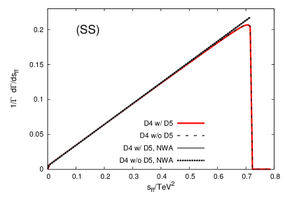
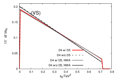
Figure 2: Differential decay rate over the invariant mass $s_{ff}$ for dim-4 couplings only (black) and including additional dim-5 (red/grey) couplings for intermediate fermions/bosons (first two row/last row). The lines correspond to: full red lines: exact spectra including dim-4 and dim-5 operators, dashed lines: exact spectra taking dim-4 operators only, full grey lines: spectra including dim-4 and dim-5 operators using NWA, dotted lines: exact spectra taking dim-4 operators only using NWA.

We show for each decay the complete dim-4 (black dashed) and dim-5 distribution (red solid) and for comparison the NWA results (dim-4 , NWA: black dotted; dim-5 , NWA: grey solid). For all decays, the NWA result is a very good approximation for the complete decays including off-shell effects. The main differences are at the kinematical endpoints. The influence of the dim-5 operators in this mass/coupling scenario is the largest in the $(FF)_{V}$ followed by the $(VS)$ decay. The first one is because in this case we have the highest power in $s_{ff}$, see eq. (3), and is a quite generic feature. The second case depends much stronger on the couplings and masses of the scenarios considered. For completeness we note, that for $(FF)_{S}$ no changes are visible when comparing the cases with and without dim-5 operators, because we show the normalized distributions.

5 Discussion and conclusions

The determination of spins of new particles is an important task at the LHC once an extension of the SM is discovered. In this way one can also discriminate between model classes, e.g. between supersymmetry and extra dimensions. In case that there are two subsequent two-body decays involving two SM fermions one can show that the spin of the intermediate particle reflects itself as in the highest power of $s_{ff}$ in the differential decay width $d\Gamma/ds_{ff}$.

There are two main theoretical uncertainties in this kind of considerations: real emission of photons and gluons in the decays. These can be calculated once the quantum numbers of the new particles are know. The second class are higher than dim-4 operators which are induced by particles close to the LHC reach. In this paper we have shown that such operators do not induce higher powers of $s_{ff}$ in the partial width and thus the existing analyses are valid even if such operators are numerically important. However, their presence can change the exact form of the slope considerably as we have seen in a concrete example. This potentially affects the determination of the underlying parameters.

Appendix

As an example for the NWA result of the decays including anomalous couplings, we give here the decay width for $S\rightarrow f\bar{f}S$. We used the following short forms for the couplings from eq. 14 and the masses used

$$\tau_{I}=\frac{m_{I}}{m_{X}}; \tau_{y}=\frac{m_{y}}{m_{x}}; 1/\Lambda_{i}=R_{i}=\frac{R^{\prime}_{i}}{m_{x}};$$

$$g_{V}=g_{r}+g_{l}; g_{A}=g_{r}-g_{l}; n_{V}=n_{r}+n_{l}; n_{A}=n_{r}-n_{l};$$

and analogous for $a_{l/r},b_{l/r},c_{l/r},x_{l/r},y_{l/r},z_{l/r}$. The NWA result in terms of these is:

$$\frac{d~{}\Gamma}{d~{}s_{ff}}=\frac{1}{(2\pi)^{3}}\frac{1}{32m_{X}}\frac{1}{m_{I}\Gamma_{I}}\left((A_{D4}+A_{D5})+s_{ff}\cdot(B_{D4}+B_{D5})\right)$$

with

$$A_{D4}= 2m_{X}^{2}\left(1-\tau_{I}^{2}\right)(\tau_{I}^{2}-\tau_{Y}^{2})\left(\left(g_{A}^{2}+g_{V}^{2}\right)\left(n_{A}^{2}+n_{V}^{2}\right)+4g_{A}g_{V}n_{A}n_{V}\right);$$

$$B_{D4}= -16g_{A}~{}g_{V}~{}n_{A}~{}n_{V}~{}\tau_{I}^{2};$$

$$A_{D5}= -2m_{X}^{2}\tau_{I}^{2}\left(\tau_{I}^{2}-1\right)(\tau_{I}^{2}-\tau_{Y}^{2})\times\left[a_{A}^{2}R^{{}^{\prime}2}_{a}\Bigl{(}n_{A}^{2}+n_{V}^{2}\right.$$

$$\left.\left.+\tau_{I}^{2}\left(R^{{}^{\prime}2}_{x}\left(x_{A}^{2}+x_{V}^{2}\right)-2R^{\prime}_{x}R^{\prime}_{z}(x_{A}z_{A}+x_{V}z_{V})+R^{{}^{\prime}2}_{z}\left(z_{A}^{2}+z_{V}^{2}\right)\right)\right)\right.$$

$$\left.+2a_{A}R^{\prime}_{a}\left(\tau_{I}^{2}\Bigl{(}2(a_{V}R^{\prime}_{a}-c_{V}R^{\prime}_{c})(R^{\prime}_{x}x_{A}-R^{\prime}_{z}z_{A})(R^{\prime}_{x}x_{V}-R^{\prime}_{z}z_{V})\right.\right.$$

$$\left.\left.\left.-c_{A}R^{\prime}_{c}\left(R^{{}^{\prime}2}_{x}\left(x_{A}^{2}+x_{V}^{2}\right)-2R^{\prime}_{x}R^{\prime}_{z}(x_{A}z_{A}+x_{V}z_{V})+R^{{}^{\prime}2}_{z}\left(z_{A}^{2}+z_{V}^{2}\right)\right)\right)\right.\right.$$

$$\left.+2a_{V}n_{A}n_{V}R^{\prime}_{a}-R^{\prime}_{c}\left(c_{A}\left(n_{A}^{2}+n_{V}^{2}\right)+2c_{V}n_{A}n_{V}\right)\Bigr{)}\right.$$

$$\left.+\tau_{I}^{2}\left[a_{V}^{2}R^{{}^{\prime}2}_{a}\left(R^{{}^{\prime}2}_{x}\left(x_{A}^{2}+x_{V}^{2}\right)-2R^{\prime}_{x}R^{\prime}_{z}(x_{A}z_{A}+x_{V}z_{V})+R^{{}^{\prime}2}_{z}\left(z_{A}^{2}+z_{V}^{2}\right)\right)\right.\right.$$

$$-2a_{V}R^{\prime}_{a}R^{\prime}_{c}\Bigr{(}2c_{A}(R^{\prime}_{x}x_{A}-R^{\prime}_{z}z_{A})(R^{\prime}_{x}x_{V}-R^{\prime}_{z}z_{V})$$

$$\left.\left.\left.+c_{V}\left(R^{{}^{\prime}2}_{x}\left(x_{A}^{2}+x_{V}^{2}\right)-2R^{\prime}_{x}R^{\prime}_{z}(x_{A}z_{A}+x_{V}z_{V})+R^{{}^{\prime}2}_{z}\left(z_{A}^{2}+z_{V}^{2}\right)\right)\right)\right.\right.$$

$$\left.\left.+R^{{}^{\prime}2}_{c}\left((c_{A}^{2}+c_{V})^{2}\left(R^{{}^{\prime}2}_{x}\left(x_{A}^{2}+x_{V}^{2}\right)-2R^{\prime}_{x}R^{\prime}_{z}(x_{A}z_{A}+x_{V}z_{V})+R^{{}^{\prime}2}_{z}\left(z_{A}^{2}+z_{V}^{2}\right)\right)\right.\right.\right.$$

$$+4c_{A}c_{V}(R^{\prime}_{x}x_{A}-R^{\prime}_{z}z_{A})(R^{\prime}_{x}x_{V}-R^{\prime}_{z}z_{V})\Bigr{)}\Bigr{]}$$

$$+a_{V}^{2}n_{A}^{2}R^{{}^{\prime}2}_{a}+a_{V}^{2}n_{V}^{2}R^{{}^{\prime}2}_{a}-4a_{V}c_{A}n_{A}n_{V}R^{\prime}_{a}R^{\prime}_{c}$$

$$-2a_{V}c_{V}n_{A}^{2}R^{\prime}_{a}R^{\prime}_{c}-2a_{V}c_{V}n_{V}^{2}R^{\prime}_{a}R^{\prime}_{c}$$

$$+c_{A}^{2}n_{A}^{2}R^{{}^{\prime}2}_{c}+c_{A}^{2}n_{V}^{2}R^{{}^{\prime}2}_{c}+4c_{A}c_{V}n_{A}n_{V}R^{{}^{\prime}2}_{c}+c_{V}^{2}n_{A}^{2}R^{{}^{\prime}2}_{c}+c_{V}^{2}n_{V}^{2}R^{{}^{\prime}2}_{c}$$

$$\left.+(g_{A}^{2}+g_{v}^{2})\left(R^{{}^{\prime}2}_{x}\left(x_{A}^{2}+x_{V}^{2}\right)-2R^{\prime}_{x}R^{\prime}_{z}(x_{A}z_{A}+x_{V}z_{V})+R^{{}^{\prime}2}_{z}\left(z_{A}^{2}+z_{V}^{2}\right)\right)\right.$$

$$+4g_{A}g_{V}(R^{\prime}_{x}x_{A}-R^{\prime}_{z}z_{A})(R^{\prime}_{x}x_{V}-R^{\prime}_{z}z_{V})\Bigr{]};$$

$$B_{D5}= -16\tau_{I}^{4}\left((a_{A}R^{\prime}_{a}-c_{A}R^{\prime}_{c})(a_{V}R^{\prime}_{a}-c_{V}R^{\prime}_{c})\left(n_{A}n_{V}\right.\right.$$

$$\left.\left.+\tau_{I}^{2}(R^{\prime}_{x}x_{A}-R^{\prime}_{z}z_{A})(R^{\prime}_{x}x_{V}-R^{\prime}_{z}z_{V})\right)\right.$$

$$\left.+g_{A}g_{V}(R^{\prime}_{x}x_{A}-R^{\prime}_{z}z_{A})(R^{\prime}_{x}x_{V}-R^{\prime}_{z}z_{V})\right).$$

References

• [1] S.Y. Choi, D.J. Miller, M.M. Mühlleitner, and P.M. Zerwas. Identifying the Higgs spin and parity in decays to Z pairs. Phys.Lett., B553:61–71, 2003.
• [2] Alexandre Alves, O.J.P. Eboli, M.C. Gonzalez-Garcia, and J.K. Mizukoshi. Deciphering the spin of new resonances in Higgsless models. Phys.Rev., D79:035009, 2009.
• [3] P. Osland, A.A. Pankov, N. Paver, and A.V. Tsytrinov. Spin identification of the Randall-Sundrum resonance in lepton-pair production at the LHC. Phys.Rev., D78:035008, 2008.
• [4] P. Osland, A.A. Pankov, A.V. Tsytrinov, and N. Paver. Spin and model identification of Z’ bosons at the LHC. Phys.Rev., D79:115021, 2009.
• [5] O. J. P. Eboli, C. S. Fong, J. Gonzalez-Fraile and M. C. Gonzalez-Garcia, Phys. Rev.  D 83 (2011) 095014 [arXiv:1102.3429 [hep-ph]].
• [6] A.J. Barr. Measuring slepton spin at the LHC. JHEP, 0602:042, 2006.
• [7] Jennifer M. Smillie and Bryan R. Webber. Distinguishing Spins in Supersymmetric and Universal Extra Dimension Models at the Large Hadron Collider. JHEP, 10:069, 2005.
• [8] Christiana Athanasiou, Christopher G. Lester, Jennifer M. Smillie, and Bryan R. Webber. Distinguishing spins in decay chains at the Large Hadron Collider. JHEP, 08:055, 2006.
• [9] Jennifer M. Smillie. Spin correlations in decay chains involving W bosons. Eur.Phys.J., C51:933–943, 2007.
• [10] Lian-Tao Wang and Itay Yavin. Spin Measurements in Cascade Decays at the LHC. JHEP, 04:032, 2007.
• [11] Patrick Meade and Matthew Reece. Top partners at the LHC: Spin and mass measurement. Phys.Rev., D74:015010, 2006.
• [12] Can Kilic, Lian-Tao Wang, and Itay Yavin. On the existence of angular correlations in decays with heavy matter partners. JHEP, 0705:052, 2007.
• [13] Alexandre Alves and Oscar Eboli. Unravelling the sbottom spin at the CERN LHC. Phys.Rev., D75:115013, 2007.
• [14] Arvind Rajaraman and Bryan T. Smith. Determining Spins of Metastable Sleptons at the Large Hadron Collider. Phys.Rev., D76:115004, 2007.
• [15] Won Sang Cho, Kiwoon Choi, Yeong Gyun Kim, and Chan Beom Park. M(T2)-assisted on-shell reconstruction of missing momenta and its application to spin measurement at the LHC. Phys.Rev., D79:031701, 2009.
• [16] Lian-Tao Wang and Itay Yavin. A Review of Spin Determination at the LHC. Int. J. Mod. Phys., A23:4647–4668, 2008.
• [17] Michael Burns, Kyoungchul Kong, Konstantin T. Matchev, and Myeonghun Park. A General Method for Model-Independent Measurements of Particle Spins, Couplings and Mixing Angles in Cascade Decays with Missing Energy at Hadron Colliders. JHEP, 0810:081, 2008.
• [18] Alan J. Barr and Christopher G. Lester. A Review of the Mass Measurement Techniques proposed for the Large Hadron Collider. J. Phys., G37:123001, 2010.
• [19] C. W. E. Chiang, N. D. Christensen, G. J. Ding and T. Han, arXiv:1107.5830 [hep-ph].
• [20] Gordon L. Kane, Alexey A. Petrov, Jing Shao, and Lian-Tao Wang. Initial determination of the spins of the gluino and squarks at LHC. J.Phys.G, G37:045004, 2010.
• [21] Csaba Csaki, Johannes Heinonen, and Maxim Perelstein. Testing Gluino Spin with Three-Body Decays. JHEP, 10:107, 2007.
• [22] Lisa Edelhäuser, Werner Porod, and Ritesh K. Singh. Spin Discrimination in Three-Body Decays. JHEP, 1008:053, 2010.
• [23] A. J. Barr. Using lepton charge asymmetry to investigate the spin of supersymmetric particles at the LHC. Phys. Lett., B596:205–212, 2004.
• [24] B.C. Allanach, C.G. Lester, Michael Andrew Parker, and B.R. Webber. Measuring sparticle masses in nonuniversal string inspired models at the LHC. JHEP, 0009:004, 2000.
• [25] H. E. Haber, “Spin formalism and applications to new physics searches,” arXiv:hep-ph/9405376.
• [26] E. Leader. Spin in particle physics. Camb.Monogr.Part.Phys.Nucl.Phys.Cosmol., 15:1, 2001.
• [27] Fawzi Boudjema and Ritesh K. Singh. A Model independent spin analysis of fundamental particles using azimuthal asymmetries. JHEP, 0907:028, 2009.
• [28] D.M Brink and G.R. Satchler. Angular momentum. Oxford University Press, London U.K., 1968.
• [29] C.F. Uhlemann and N. Kauer. Narrow-width approximation accuracy. Nucl.Phys., B814:195–211, 2009.
• [30] K. Nakamura et al. Review of particle physics. J.Phys.G, G37:075021, 2010.
• [31] W. Buchmüller and D. Wyler. Effective Lagrangian Analysis of New Interactions and Flavor Conservation. Nucl. Phys., B268:621, 1986.