XUV frequency comb metrology on the ground state of helium

Abstract

The operation of a frequency comb at extreme ultraviolet (XUV) wavelengths based on pair-wise amplification and nonlinear upconversion to the $15^{th}$ harmonic of pulses from a frequency comb laser in the near-infrared range is reported. Following a first account of the experiment [Kandula et al., Phys. Rev. Lett. 105, 063001 (2010)], an extensive review is given of the demonstration that the resulting spectrum at 51 nm is fully phase coherent and can be applied to precision metrology. The pulses are used in a scheme of direct-frequency-comb excitation of helium atoms from the ground state to the $1s4p$ and $1s5p$ ¹P₁ states. Laser ionization by auxiliary $1064$ nm pulses is used to detect the excited state population, resulting in a cosine-like signal as a function of the repetition rate of the frequency comb with a modulation contrast of up to 55%. Analysis of the visibility of this comb structure, thereby using the helium atom as a precision phase ruler, yields an estimated timing jitter between the two upconverted comb laser pulses of 50 attoseconds, which is equivalent to a phase jitter of $0.38(6)$ cycles in the XUV at $51$ nm. This sets a quantitative figure of merit for the operation of the XUV comb, and indicates that extension to even shorter wavelengths should be feasible. The helium metrology investigation results in transition frequencies of $5740806993(10)$ MHz and $5814248672(6)$ MHz for excitation of the $1s4p$ and $1s5p$ ¹P₁ states, respectively. This constitutes the first absolute frequency measurement in the XUV, attaining unprecedented accuracy in this windowless part of the electromagnetic spectrum. From the measured transition frequencies an eight-fold improved ⁴He ionization energy of $5945204212(6)$ MHz is derived. Also a new value for the ⁴He ground state Lamb shift is found of $41247(6)$ MHz. This experimental value is in agreement with recent theoretical calculations up to order $m\alpha^{6}$ and $m^{2}/M\alpha^{5}$, but with a six times higher precision, therewith providing a stringent test of quantum electrodynamics in bound two-electron systems.

I Introduction

Atomic spectroscopy has been paramount for the discovery of the laws of physics. The ordering of spectral lines in the hydrogen atom has led to the Rydberg formula and the concept of quantization in the old Bohr model led eventually to the formulation of quantum mechanics. In 1947 further advance was made with the observation by Lamb and Retherford that the $2^{2}\mathrm{S}_{1/2}$ and $2^{2}\mathrm{P}_{1/2}$ states in hydrogen are not degenerate, but differ by 1 GHz Lamb and Retherford (1947, 1950). This result lead to the development of quantum electrodynamics (QED) Feynman (1949); Schwinger (1948); Tomonaga (1946), which is the most precisely tested physics theory to date. Since the first measurement by Lamb and Retherford, QED contributions to energy levels in atoms are referred to as “Lamb shifts”. The theory has been elaborately tested and confirmed by experiments in various bound systems, ranging from atomic hydrogen Huber et al. (1999); Parthey et al. (2010), via one-electron heavy-ion systems Gumberidze et al. (2005), exotic atomic systems such as positronium Hagena et al. (1993) and muonium Meyer et al. (2000) to one-electron molecular ions Korobov et al. (2009); Koelemeij et al. (2007), while recently a test of the QED has also been reported in a neutral molecule Salumbides et al. (2011). Tests have also been performed on the anomalous magnetic dipole moment of the electron (“g-2”), so that in fact QED can now be used to derive a new value for the fine structure constant from such a measurement Hanneke et al. (2008).

The two main QED contributions to the energy of an atomic system are virtual photon interactions (”self energy”) and screening of the nuclear charge due to the creation (and annihilation) of electron-positron pairs (”vacuum polarization”). The magnitude of these effects depends on the considered system and its energy eigenstate, and is studied by means of precision spectroscopy. In atoms such as hydrogen and helium, the strongest QED effects are observed in the electronic ground states. For this reason spectroscopy involving the ground state is preferred. In the case of hydrogen this is achieved by inducing a two-photon transition at 2 $\times$ 243 nm from the $\mathrm{1S}$ ground state to the $\mathrm{2S}$ excited state, which has reached a level of precision that allows a detailed comparison between theory and experiment Fischer et al. (2004). This comparison is currently limited by the uncertainty in the measured proton charge radius Pachucki and Jentschura (2003); Fischer et al. (2004); Pohl et al. (2010), which in itself is not a QED phenomenon. Assuming that the QED calculations are correct, one can also use the $\mathrm{1S-2S}$ experiment in hydrogen to determine the effective proton charge radius. In this respect it is interesting to note that a recent experiment with muonic hydrogen (where the electron in hydrogen is replaced by a muon), has resulted in a proton size that differs 5$\sigma$ Pohl et al. (2010) with the CODATA value that is based mainly on hydrogen spectroscopy. The origin of this difference is still under debate Jentschura (2011); De Rujula (2011); Cloet and Miller (2011); Barger et al. (2011).

In principle a more stringent test of QED could be performed by experiments using atoms with a higher nuclear charge $Z$, as the non-trivial QED effects scale with $Z^{4}$ and higher. For this reason experiments have been performed on many different high-$Z$ ionic species such as $\mathrm{U}^{91+}$ Gumberidze et al. (2005). However, the required (very) short wavelengths for excitation, such as hard-X-rays, makes it very difficult to perform absolute frequency measurements (see e.g. Epp et al. (2010) and references therein).

Even for $Z=2$ in the He⁺ ion or the neutral helium atom, where QED effects are at least 16 times larger than in hydrogen, it remains difficult to perform high resolution spectroscopy. In the case of He⁺ a two-photon excitation from the ground state requires 60 nm, while for neutral helium 120 nm is required to drive the $1s^{2}$ ${}^{1}\mathrm{S}_{0}-1s2s$ ${}^{1}\mathrm{S}_{0}$ two-photon transition. One-photon transitions require even shorter wavelengths, in the extreme ultraviolet (XUV), e.g. $58$ nm to excite the $1s^{2}$ ${}^{1}\mathrm{S}_{0}-1s2p$ ${}^{1}\mathrm{P}_{1}$ first resonance line in neutral helium.

A major obstacle to precision spectroscopy in the XUV is the lack of continuous wave (CW) narrow bandwidth laser radiation. Instead pulsed-laser techniques have been used. The first laser-based measurement of the $1s^{2}$ ${}^{1}\mathrm{S}_{0}-1s2p$ ${}^{1}\mathrm{P}_{1}$ resonance line at $58.4$ nm was achieved via upconversion of the output of a grating-based pulsed dye laser Eikema et al. (1993). Subsequently, pulsed amplification of CW lasers and harmonic generation in crystals and gases led to production of narrower bandwidth XUV radiation. In this fashion spectroscopy on neutral helium has been performed from the ground state using ns-timescale single pulses of 58.4 nm Eikema et al. (1997, 1996). In an alternative scheme two-photon laser excitation of neutral helium at 120 nm was achieved Bergeson et al. (1998, 2000). In both experiments transient effects resulted in ”frequency chirping” of the generated XUV pulses, which limited the accuracy of the spectroscopy to about 50 MHz.

Here we overcome this problem by exciting transitions using a pair of phase coherent XUV pulses, produced by amplification and high-harmonic generation (HHG) of pulses from a frequency comb laser. In such a scheme most of the nonlinear phase shifts and those due to short-lived transients cancel as only differential pulse distortions enter the spectroscopic signal. In effect, a frequency comb in the XUV is generated. The employed method of spectroscopy with this XUV comb laser is a form of Ramsey spectroscopy Ramsey (1949). Early experiments using phase-coherent pulse excitation in the visible part of the spectrum used a delay line Salour and Cohen-Tannoudji (1977), a resonator Teets et al. (1977) or modelocked lasers Eckstein et al. (1978) to create two or more phase-coherent pulses. More recently, amplified ultrafast pulses have been split using a Michelson interferometer or other optical means to create two coherent XUV pulses after HHG Salieres et al. (1999); Bellini et al. (2001); Kovačev et al. (2005). Coherent excitation of argon in the XUV with a delay of up to $\approx$100 ps Liontos et al. (2010) has been demonstrated in this manner. However, with these methods no absolute calibration in the XUV has been demonstrated up to now as it is very difficult to calibrate the time delay and phase difference between the pulses with sufficient accuracy. In the present experiment we use a frequency comb laser (FCL) Diddams et al. (2000); Holzwarth et al. (2000) to obtain phase-coherent pulses in the XUV which allows for a much higher resolution and immediate absolute calibration.

Single femtosecond laser pulses can be made sufficiently intense for convenient upconversion to XUV or even soft x-ray frequencies using HHG Seres et al. (2005). However, as a consequence of the Fourier principle, the spectral bandwidth of such pulses is so large that it inhibits high spectral resolution. Frequency combs combine high resolution with high peak power by generating a continuous train of femtosecond pulses. In this case the spectrum of the pulse train exhibits narrow spectral components (modes) within the spectral envelope determined by the spectrum of a single pulse. The modes are equally spaced in frequency at positions given by:

$$f_{n}=nf_{rep}+f_{CEO}$$ (1)

were $n$ denotes the integer mode number, $f_{rep}$ is the repetition frequency of the pulses, and $f_{CEO}$ is the carrier-envelope offset frequency. The latter relates to the pulse-to-pulse phase shift $\Delta\phi_{CE}$ between the carrier wave and the pulse envelope (carrier-envelope phase or CEP) by

$$\Delta\phi_{CE}=2\pi f_{CEO}/f_{rep}.$$ (2)

Each of the comb modes can be used as a high-resolution probe almost as if it originated from a continuous single-frequency laser Fendel et al. (2007); Marian et al. (2005); Wolf et al. (2009). If the entire pulse train can be phase coherently upconverted, the generated harmonics of the central laser frequency should exhibit a similar spectrum with comb frequencies $mf_{rep}+qf_{CEO}$ , where $m$ denotes again an integer mode number, and $q$ is the integer harmonic order under consideration. By amplification of a few pulses from the train, and producing low harmonics in crystals and gases, an upconverted comb structure has been demonstrated down to $125$ nm Witte et al. (2005); Zinkstok et al. (2006). However, to reach wavelengths below $120$ nm, HHG has to be employed requiring nonlinear interaction at higher intensities in the non-perturbative regime Lewenstein et al. (1994). It is well established that HHG can be phase coherent to some degree Salieres et al. (1999); Bellini et al. (2001); Cavalieri et al. (2002); Lewenstein et al. (1994); Zerne et al. (1997); Liontos et al. (2010), and attempts have been made to generate frequency combs based on upconversion of all pulses at full repetition rate Gohle et al. (2005); Jones et al. (2005); Ozawa et al. (2008); Yost et al. (2009). However, due to the low XUV-pulse energies the comb structure could so far not be verified in the XUV-domain for those sources. That limitation can be overcome by combining parametric amplification of two frequency comb pulses in combination with harmonic upconversion. This was recently demonstrated with direct frequency comb excitation at $51$ nm in helium Kandula et al. (2010), and in this paper a full and detailed description is given of that experiment.

The article is organized as follows: in section II the measurement principle is explained, followed in section III with a description of the different parts of the experimental setup. The general measurement procedure and results are presented in section IV. In section V, part A, a discussion of all systematic effects that need to be taken into account to determine the ground state ionization potential from the measured transitions frequencies is given. This is followed in part B with a discussion of the timing jitter in the XUV, which can be derived from the measured Ramsey signal. In the final section VI the conclusions and an outlook are presented.

II Overview and principle of XUV comb generation and excitation

A frequency comb is normally based on a modelocked laser producing an infinite train of pulses with fixed repetition rate and CEP-slip between consecutive pulses. The corresponding spectrum of such a pulse train consists of a comb of narrow optical modes associated with frequencies given by Eq. 1. To convert the frequency comb to the XUV, we select only two pulses from the FCL. In this case the spectrum changes to a cosine-modulated continuum, but with the peaks of the modulation exactly at the positions of the original FCL spectrum. This “broad frequency comb” is converted in a phase-coherent manner to the XUV by amplification of the pulse pair to the millijoule level, and subsequent HHG. Once the FCL pulses (separated by the time $T=1/f_{rep}$) are upconverted, they can be used to directly probe transitions in atoms or molecules. This form of excitation with two pulses resembles an optical (XUV) version of the Ramsey method of spatially (and temporally) separated oscillatory fields Ramsey (1949); Witte et al. (2005). In the present case, the interacting fields are not separated in space, but only in time. Excitation with two (nearly) identical pulses produces a signal which is cosine-modulated according to:

$$S(T)\propto cos(2\pi(f_{tr}T)-\Delta\phi(f_{tr}))$$ (3)

when varying $T$ through adjustment of $f_{rep}$ of the comb laser. In this expression $f_{tr}$ is the transition frequency and $\Delta\phi(f_{tr})$ is the spectral phase difference at the transition frequency between the two pulses. Relation (3) is valid only for weak interaction, which is the case in the current experiment given an excitation probability of $\ll 1$ per atom.

Without HHG and in the absence of additional pulse distortions the phase shift $\Delta\phi:=\Delta\phi(f_{tr})$ is equal to $\Delta\phi_{CE}$. The excitation signal will exhibit maxima corresponding to those frequencies where the modes of the original comb laser come into resonance with the transition.

The spectral phase difference of the generated XUV pulse pair cannot be determined directly. Therefore we need to propagate the spectral phase difference from the frequency comb through the parametric amplifier and the HHG process into the interaction region. The phase shift $\Delta\psi(f)$ imprinted on the pulses by the non-collinear optical parametric double-pulse amplifier (NOPCPA) is measured direcly using an interferometric technique described previously Kandula et al. (2008). To model the HHG process we employ a slowly varying envelope approximation described in section V, which yields a differential XUV phase shift of the form

$$\Delta\phi_{q}=q(\Delta\phi_{CE}+\overline{\Delta\psi})+\Delta\psi_{q},$$ (4)

where $\overline{\Delta\psi}$ denotes the carrier envelope phase accumulated in the NOPCPA (compare Sec. IV), $q$ is the harmonic order of the resonant radiation and $\Delta\psi_{q}$ is an additional phase shift due to nonlinear and transient response in the HHG process Lewenstein et al. (1995); Pirri et al. (2007) and transient effects such as ionization. Note that only differences in phase distortion between the two subsequent pulses from the FCL affect $\Delta\phi_{q}$ and therefore the Ramsey signal. Shared distortions, such as frequency chirping due to uncompensated time-independent dispersion, have no influence on the outcome of this experiment.

The frequency accuracy of the method scales with the period of the modulation ($f_{rep}$, here equal to $100-185$ MHz) rather than the spectral width of the individual pulses (about $7$ THz in the XUV at the $15^{th}$ harmonic). An error $\delta$ in the value of $\Delta\phi_{q}$ leads to a frequency error in the spectroscopy result of $\Delta f=\delta/(2\pi T)$. Of the two components contributing to this error, $\Delta\psi(f)$ can be expected to be independent of $T$, while the transients contained in $\Delta\psi_{q}$ decay with increasing $T$. Therefore $\Delta f$ decreases at least with $1/T$, leading to a higher accuracy for a longer time separation between the pulses. In practice there is still a minimum requirement on the stability and measurement accuracy of phase shift of rms 1/200th of a cycle (at the fundamental frequency of the FCL in the near infrared). This ensures that the contribution $\overline{\delta\psi}$ to the frequency uncertainty of the measured transition frequency is small enough so that the ’mode number’ ambiguity in the transition frequency, due to the periodicity of the signal, can be resolved with confidence.

A sketch of the XUV comb principle in the frequency domain is shown in Fig. 1. A FCL serves as a source of phase-coherent pulses. A pair of such pulses is amplified in a NOPCPA to the mJ level, yielding a cosine modulated spectrum when viewed in the frequency domain. The amplified pulses are filtered spatially with two pinholes, one placed between the second and third amplification stage, and one after compression respectively. As a result the pulse pairs show less spatial intensity and phase variation compared to the unfiltered beam.

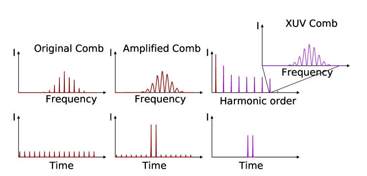
Figure 1: Principle of frequency comb generation and spectroscopy in the XUV. (a) Schematic of the spectral and temporal structure of the generated light at the different stages in the experiment (left to right): sharp equidistant frequencies from the infrared FC laser, followed by double-pulse amplification resulting in a cosine modulated spectrum, and finally HHG resulting in odd harmonics of the central frequency, where each of the harmonics consist of a XUV comb in the form of a cosine-modulated spectrum with period $f_{rep}$.

Before the IR beam is focused in a krypton jet for HHG, the center of it is blocked by a $1.9$ mm diameter copper disk, while the outside is clipped with an iris. The donut-mode shape is used to facilitate the separation of the driving IR field from the generated XUV emitted on axis (see also section III.4).

Phase shifts in the NOPCPA, which are not common for both pulses, and therefore change the position of the comb modes, are measured by means of spectral interference. A Mach-Zehnder-like configuration is used to interfere the original comb pulses with those that are amplified by the NOPCPA, as described in Kandula et al. (2008) and section III.3.

The amplified pulses are focused a few mm in front of a krypton jet, in which two phase-locked pulses of high-order harmonics are generated to create a cosine-modulated comb spectrum in the XUV. In order to avoid direct ionization of helium with higher-order harmonics, the IR intensity in the interaction region and the harmonic medium are chosen such that the desired $15^{th}$ harmonic appears at the cutoff of the HHG process. The XUV beam crosses a low-divergence beam of helium atoms perpendicularly, and excites them from the ground state to the $1snp$ ${}^{1}\mathrm{P}_{1}$ state ($n\in\{4,5\}$). A pulse of $1064$ nm radiation ionizes the excited atoms, which are subsequently detected in a time-of-flight mass spectrometer. Tuning of the XUV comb is accomplished by changing $f_{rep}$ of the FCL. The changing mode separation effectively causes the modes in the XUV to scan over the transition. An example for a scan of the repetition time corresponding to approximately $500$ attoseconds (as) is shown in Fig. 2. The number $m$ of the mode that excites the measured transition in this experiment is in the order of $50$ million. This means that the repetition rate of the fundamental FCL needs to be changed only by a few Hz in order to bring an adjacent XUV-mode $f_{m\pm 1}$ into resonance with a helium transition ($f_{m}$ is assumed to be at the transition initially). As a consequence the ionization signal will be cosine modulated. In order to resolve the resulting ambiguity in the mode-number assignment, the measurement is repeated with different repetition rates, corresponding to pulse delays between $5.4$ ns and $10$ ns.

Besides the frequency-domain perspective, this experiment can be viewed also in the time domain. In this case it can be seen as a pump-probe experiment, which tracks the dynamics of the electronic wave function that results from mixing the ground state of helium with the excited $p$-level. The first XUV pulse brings the atom into a superposition of the ground and the excited state. This superposition results in a dipole, which oscillates at the transition frequency with an amplitude that decays according to the lifetime of the excited state. The second pulse probes this oscillation. Two extreme cases can be distinguished. If the second pulse is in phase with the dipole oscillation, the amplitude of the excited state increases, and thus its detection probability. If the phase of the second pulse is shifted by $\pi$ with respect to the dipole oscillation of the helium atom, its oscillatory movement is suppressed and the probability to find an atom in the excited state is decreased.

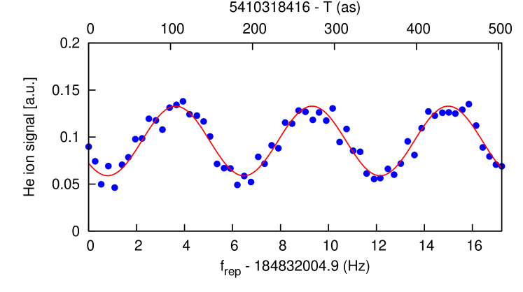
Figure 2: The excitation probability of helium at $51.5$ nm on the $1s^{2}$ ${}^{1}\mathrm{S}_{0}-1s5p$ ${}^{1}\mathrm{P}_{1}$ transition, as a function of the repetition of the frequency comb laser (lower x-axis), and the delay between the pulses (upper x-axis in attoseconds). In this example $f_{CEO}$ is locked $46.21$ MHz, and a 1:5 He:Ne mixture is used for the atomic beam.

III Experimental setup

The measurement setup consists of four major elements: a frequency comb laser, a non-collinear parametric amplifier, a phase-measurement system, and a vacuum apparatus for HHG and excitation of helium in an atomic beam. A schematic overview of the setup is given in Fig. 3.

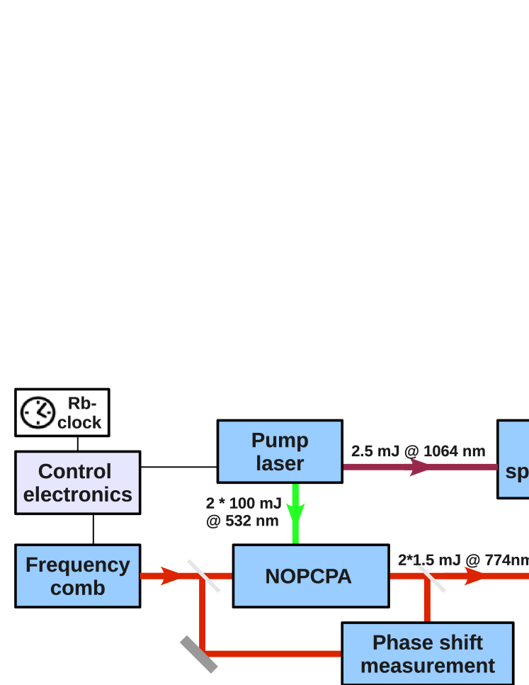
Figure 3: Scheme of the experimental setup, including: femtosecond frequency comb laser with control electronics, non-collinear optical parametric chirped-pulse amplifier (NOPCPA), a phase measurement in a Mach-Zehnder interferometer, high harmonic generation (HHG) and a spectroscopy apparatus. Part of the pump laser output at $1064$ nm is used as ionization beam.

III.1 Frequency-comb oscillator and pulse stretcher

Phase-coherent pulses are obtained from a home-built Kerr-lens mode-locked Ti:Sapphire frequency comb laser. The FCL has an adjustable repetition rate between $100$ MHz and $185$ MHz. Dispersion compensation in the cavity is obtained with a set of chirped mirrors, supporting a spectral bandwidth of $60$ nm centered around $780$ nm. The FCL is stabilized and calibrated against the signal of a rubidium clock (Stanford research PRS10), which itself is referenced to a GPS receiver so that an accuracy on the order of $10^{-11}$ is reached after a few seconds of averaging. Before sending the FCL pulses to the amplifier, the wavelength and bandwidth of the comb pulses is adjusted with a movable slit in the Fourier plane of a grating-based $4-f$ stretcher ($1200$ l/mm, $f=10$ cm). The bandwidth is set to $6$ nm in this device, ensuring that after upconversion to the XUV only one state in helium is excited at a time. The spectral clipping and losses from the gratings in the stretcher reduce the pulse energy from about $5$ nJ to $60$ pJ. At the same time the added dispersion and reduced bandwidth lengthens the pulse to about $2$ ps.

III.2 Non-collinear optical parametric amplifier

A pair of subsequent pulses obtained from the stretcher is amplified in a non-collinear optical parametric chirped-pulse amplifier based on two $5$ mm long BBO (beta-barium borate) crystals. Here we present a concise description of the system, while further details can be found in Kandula et al. (2008); Witte et al. (2006). The amplifier operates at a repetition rate of $28$ Hz, and amplifies two subsequent FC pulses to a level of typically $5$ mJ each. The bandwidth of the pulses remains essentially unchanged compared to that selected by the slit of the preceding stretcher, although saturation effects in the NOPCPA result in a ’cathedral’-like spectrum (see Fig. 4). The pump light for the NOPCPA (two pulses at $532$ nm, $50$ ps, $80-100$ mJ per pulse) is obtained by frequency doubling $1064$ nm light from a Nd:YAG-based pump laser. A relay-imaged delay line in the pump laser is used to produce these pulse pairs with a time separation between $5.5$ ns and $10$ ns. This time separation is adjusted carefully for each value of $f_{rep}$ to match the time delay between consecutive pulses from the FC laser at a few-ps level.

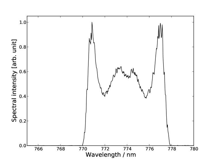
Figure 4: A typical spectrum of the pulse-pair after NOPCPA, acquired with a resolution of $0.1~{}\mathrm{nm}$ measured by an Ando AQ-6315A optical spectrum analyzer.

Electronic synchronization is employed (timing jitter less than $1$ ps) so that the pump and comb laser pulses arrive at the BBO crystals at the same time. The amplification happens in three stages, the first two located in the first BBO crystal and the last (power amplifier) stage uses the second. Between the first and second crystal spatial filtering is used to reduce phase-front errors. After amplification in the NOPCPA, and subsequent compression, a final spatial filter is employed (based on a 1:1 telescope with $f=50$ cm lenses and an $80$ micron pinhole in between, mounted in vacuum). This reduces wave-front errors and results in a Gaussian beam with a diameter of $6$ mm. The pulses of $300$ fs duration are essentially diffraction and Fourier-limited with an energy of $1-2$ mJ per pulse.

By choosing parametric amplification, a high gain ($10^{8}$) is achieved while avoiding some of the transient effects that conventional laser amplifiers suffer from, such as thermal lensing and inversion depletion. The reason for this is that in NOPCPA negligible power is dissipated in the amplifier medium (a nonlinear crystal), and that the amplified (’signal’) wave is not distorted provided the process is perfectly phase matched (see e.g. Renault et al. (2007)). Imperfections of the wave front of the pump-beam pulses can lead to a spatially-dependent phase mismatch in the NOPCPA, which in turn influences the phase of the amplified signal beam. Therefore special attention is paid to match the properties (wave front, pulse length, energy, diameter) of the two pump pulses so that induced phase effects in the two amplified signal pulses are as equal as possible. A Shack-Hartmann sensor was used to align their direction within several $\mu$rad and their propagation axis within $10~{}\mu$m. The remaining spatial differential signal distortions are reduced by the spatial filters and finally measured interferometrically as described in the next section.

III.3 Phase-shift measurements in the IR

Knowledge of the carrier-envelope phase change between consecutive pulses of a repetition-frequency stabilized mode-locked laser is a prerequisite for frequency-comb metrology. Because parametric amplification influences the phase of the amplified light Ross et al. (2002); Witte et al. (2007), a method is needed to detect a differential phase shift between the pulses. This shift is recorded for each laser shot, using spectral interferometry with the original comb pulses as a reference in a Mach-Zehnder configuration (Fig. 3).

The phase-measurement setup is an advanced version of the one published earlier Kandula et al. (2008). In order to deal with the demand for higher spectral resolution of the phase-measurement setup and the spatial dependence of the phase shift between the pulses, several improvements were made. The most important is a motorized iris (diameter: $2$ mm), which enables spatial mapping of the differential phase within 30 seconds, by scanning it along the donut mode (see also section III.4). Such a wave-front scan is made before every recording of the helium signal as it cannot be done for every individual laser shot while measuring the helium signal. However, during a recording of the helium signal the iris is opened and an average value for the shift of $\Delta\phi_{q}$ is monitored for each laser shot. This average is compared with the wave-front scan made just before a recording of the helium signal from which a correction for the average phase shift is calculated. In this way the effective phase difference change can be continuously monitored. The differential phase distortion along the donut-mode profile has a typical magnitude of $100$ mrad, and a spatial variation of $20-30$ mrad.

Perfect spatial overlap between the amplified and reference pulses is ensured by sending both beams through a $2$ meter long large-mode volume (field diameter $20$ $\mu$m) single-mode photonic fiber. Before doing so, the pulses are stretched approximately 40 times in a grating stretcher. The combination ensures that both amplified and reference beam are perfectly overlapped, while the stretching and the large mode volume of the fiber enables to increase the pulse energy for good signal-to-noise ratio without inducing self-phase modulation (SPM) in the fiber. This last aspect is particularly important because otherwise intensity differences between the pulses could induce SPM and corrupt the result of the phase shift determination.

III.4 High harmonic generation

The central part of the amplified and spatially filtered beam is blocked by a $1.9$ mm diameter copper disk to facilitate separation of the fundamental IR light and generated XUV further downstream. High harmonics are produced by focusing this donut-shaped beam ($f=500$ mm) a few mm in front of a pulsed krypton gas jet. The intensity at the focus is estimated to be less than $5\times 10^{13}$ W/cm², whle the local gas density is estimated at a few mbar. After the focus the beam encounters an iris of $0.8$ mm diameter at $40$ cm distance from the jet, which is placed in the image plane of the copper disk. The iris blocks the infrared radiation with an extinction of better than $1:27$, while the XUV light emitted on axis can freely propagate. Thereafter the XUV beam passes the interaction chamber (described below), and enters a normal-incidence focusing grating monochromator equipped with an electron multiplier to analyze the harmonic spectrum. We estimate that about $1\times 10^{8}$ photons at the $15^{th}$ harmonic at $51.5$ nm are generated per laser shot. The driving intensity is chosen on purpose at such a level that the $15^{th}$ harmonic is positioned exactly at the cut-off of the HHG process. As a result the next harmonic (the $17^{th}$, causing background counts due to direct ionization of helium atoms in the spectroscopy experiment downstream) is about $10$ times weaker.

III.5 Spectroscopy chamber

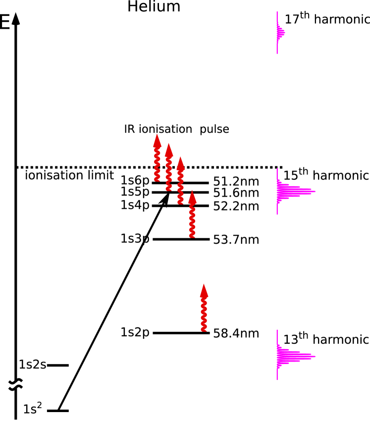
Figure 5: The XUV comb drives transitions from the $1s^{2}$ ${}^{1}\mathrm{S}_{0}$ to the $1snp$ ${}^{1}\mathrm{P}_{1}$ states with the $15^{th}$ harmonic, and excites the continuum with the $17^{th}$ and higher harmonics. The excited state population of the $1s4p$ state and above is selectively ionized using $1064$ nm radiation. Compared to this schematic, the harmonics are in reality narrower, and contain many more modes (about $50000$).

In the interaction chamber the XUV double pulse intersects a low-divergence beam of helium atoms at perpendicular angle to avoid a Doppler shift. The atomic beam is generated using a pulsed valve (General Valve, backing pressure $3$ bar) producing a supersonic expansion with either pure helium or a mixture with a noble gas (ratio $1$ He : $5$ NG). By seeding in Kr, Ar and Ne the helium velocity can be varied over a factor of $4$ to investigate Doppler effects. The divergence of the atomic beam is limited to approximately $3-4$ mrad by two skimmers: one circular skimmer of $0.3$ mm diameter and one adjustable slit skimmer of $0.25$ mm width to set the XUV-He beam angle. This divergence is similar to the divergence of the XUV beam ($<2$ mrad). Directly after interaction with the XUV-pulse pair the excited state population is detected by state-selective ionization (see Fig. 5) with a $50$ ps pulse at $1064$ nm. The resulting helium ions are detected in a time-of-flight mass spectrometer.

IV Frequency metrology on $1s^{2}-1s4p$ and $1s^{2}-1s5p$ transitions in helium

The generated XUV comb has been used to measure the $1s^{2}-1s4p$ and $1s^{2}-1s5p$ transition frequencies, from which an improved value for the helium ground state binding energy is derived. Because this involves tests of many systematic effects, a hierarchy of measurements can be identified (see table 1). The first level is that of a single recording of the helium signal as a function of the repetition rate of the frequency comb laser in the IR. To record the helium signal, the infrared FC-laser repetition frequency is scanned in steps of less than $20$ mHz, resulting in changes in the time separation between the two pulses of around $1$ attosecond. Each scan requires recording of $20000-30000$ laser pulses, which takes about $15$ minutes. For each laser shot, we record the ion signal, together with a series of other parameters, which are the frequency comb repetition frequency $f_{rep}$ and offset frequency $f_{CEO}$, the individual IR-pulse energies, energy $E_{XUV}$ of both XUV pulses and the average amplifier phase shift. The records are then binned into typically 20 groups over a Ramsey period, based on a scaled coordinate $u$ defined as

$$u:=[q(f_{CEO}+\frac{\overline{\Delta\psi}}{2\pi}f_{rep})-f_{th}]/f_{rep}$$ (5)

where $q$ is the harmonic order ($q=15$), $f_{th}$ is the theoretically predicted transition frequency, and $\overline{\Delta\psi}$ is the phase shift at the peak of the envelope, which is calculated from the phase measurement and additional corrections (see section V). We calculate the excitation probabilities $p(u)$ per laser shot, and averages of the other measured parameters within each bin, denoted by bars over the respective symbol from here on. The measured transition frequency $f_{tf}=f_{th}+f_{ex}$, average background $p_{0}$, and Ramsey-fringe amplitude $A$ are then fitting parameters in the following model:

$$p(u)=\bigg{(}p_{0}+A\cos{2\pi[u+f_{ex}/\overline{f_{rep}}(u)]}\bigg{)}/\overline{E_{XUV}(u)}$$ (6)

This results in a transition frequency $f_{ex}$ for a single scan, relative to the theoretical transition frequency $f_{th}$. The statistical error in this fit is determined via a bootstrap method Press et al. (1992), which requires no model of the noise sources.

The theoretical transition frequencies $f_{th}$, used in the fitting procedure as a reference to which the experimental value is determined, are obtained by combining recent values of the theoretical ground state energy from the literature Yerokhin and Pachucki (2010) with those of the excited states Morton et al. (2006). Predicted theoretical frequencies are $5740806963(36)$ MHz for the $1s^{2}$ ${}^{1}\mathrm{S}_{0}-1s4p$ ${}^{1}\mathrm{P}_{1}$ and $5814248632(36)$ MHz for the $1s^{2}$ ${}^{1}\mathrm{S}_{0}-1s5p$ ${}^{1}\mathrm{P}_{1}$ transitions.

In Fig. 2 a typical recording of the excitation of helium by scanning the XUV comb over the $1s^{2}$ ${}^{1}\mathrm{S}_{0}-1s5p$ ${}^{1}\mathrm{P}_{1}$ transition is shown. The contrast of the modulation (in this example $40\%$) is smaller than unity due to various effects, like Doppler broadening, frequency noise and a finite constant background of about $15\%$ due to direct ionization with the $17^{th}$ and higher harmonics. Fitting of a single recording typically shows a statistical error of $1/50$th of a modulation period. Depending on the repetition rate it amounts to an uncertainty of $2-3$ MHz, which is unprecedented in the XUV spectral region.

Several scans are then performed while changing one parameter in the setup (e.g. helium velocity) to determine the magnitude of systematic effects. Such a measurement sequence is referred to as a “series” in the following. The two most frequently performed tests (series) determine the Doppler shift (by changing the helium velocity using gas mixtures) and ionization-induced frequency shift (by varying the density in the krypton jet). Less frequently the IR-pulse ratio was also varied to test its influence on the measured transition frequency. The analysis of these tests, as well as additional experiments that have been performed to determine other systematic errors, are described in more detail in section V. Each of the series typically requires $4-6$ scans. From this data we extract (inter/extrapolate) the measured transition frequency in absence of the investigated effects and a coefficient for correcting the shifted values. For example, the extrapolation to zero velocity in a Doppler-shift measurement yields a Doppler-free frequency plus the slope, i.e. the angle between XUV and atomic beam. The angle can be used to correct the Doppler shift of scans at a finite known helium velocity. A ’session’ then consist of a number ($2-15$) of these series containing in total up to $60$ scans. Within each session, groups of series are selected so that each group contains at least one Doppler measurement and one ionization-effect measurement. If possible, also a pulse-ratio-variation measurement is included, otherwise a default dependence is used based on previous measurements.

Figure 6 gives an example for a data set acquired in a measurement session. The different series are displayed therein as red circles for Doppler-shift measurements, green triangles for ionization-shift determinations and blue squares for the measurement of the shift related to the pulse-intensity ratio. Note, that some measurements are used to derive both the Doppler and the ionization-related contribution. These separate determinations are used to mutually correct each other for the different tested aspects (so e.g. an ionization-series value is corrected for the Doppler shift measured just before or after, and vice versa). The error bar on each series depends on the statistical error of its single recordings, and the fit of the systematic effect. After grouping, a sequence of transitions frequencies results with an appropriate error bar. Additional corrections (such as Stark shift, recoil shift) are then applied, and the theoretical value for the energy of the excited state is taken into account. The weighted average over these values then leads to a session-level value for the ground state binding energy and an error estimate for it.

Each session is performed for a combination of one upper state in helium (either $4p$ or $5p$), with one repetition rate of the frequency comb laser. Most recordings were made of the $1s^{2}$ ${}^{1}\mathrm{S}_{0}-1s5p$ ${}^{1}\mathrm{P}_{1}$ transition. As an additional check also one series was measured on the $1s^{2}$ ${}^{1}\mathrm{S}_{0}-1s4p$ ${}^{1}\mathrm{P}_{1}$ transition. A weighted average over all sessions then leads to a new value for the measured transition energies.

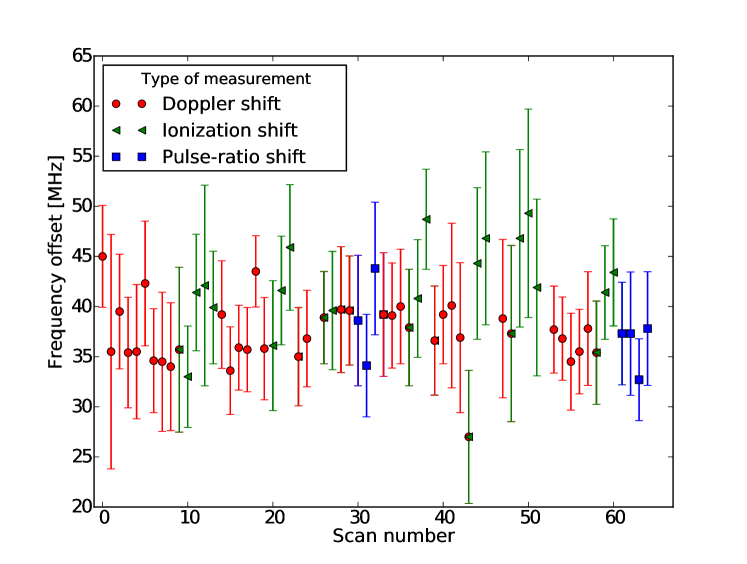
Figure 6: A measurement session performed on the $1s^{2}$ ${}^{1}\mathrm{S}_{0}-1s5p$ ${}^{1}\mathrm{P}_{1}$ transition in helium at $f_{rep}=121$ MHz. The uncorrected frequency offset from theory $f_{th}$ is displayed on the y-axis. The different shapes of the points indicate measurement series of systematic effects. Doppler-measurement series are shown as red circles, ionization shift measurement series with green triangles while the blue squares denote the measurement of pulse-intensity related effects.

V Discussion

The experiments discussed in this article yield a two-fold result. The phase coherence of the XUV-pulse pair allows to measure the frequency of an electronic transition in helium. In addition, the contrast of the Ramsey fringes, obtained for different repetition frequencies and helium velocities is used to investigate the coherence of the generated XUV radiation. Accordingly the following discussion is divided in two major parts: an evaluation of the measured transition frequencies and a contrast analysis of the observed interference signals.

V.1 Determination of the ground-state energy of helium with an XUV-frequency comb

For an absolute measurement many systematic effects have to be considered in addition to the already mentioned effects of Doppler shifts, phase shifts in the NOPCPA and in the HHG. These include recoil shifts, refractive index changes (Kerr effect) in the focusing lens for HHG and the entrance window to the vacuum setup, and the influence of the plasma generated in the HHG medium. Also AC and DC Stark effects and Zeeman shifts are considered. A new ionization energy for helium is derived from these measurements by taking the excited states ionization energy of the $4p$ and $5p$ into account. The binding energies of these states are known to an accuracy better than $20$ kHz from calculations Yerokhin and Pachucki (2010); Morton et al. (2006). From the systematic studues an improved experimental value is then obtained; an error budget for this value is listed in Table 1

To remove the ambiguity due to the periodic comb spectrum, the energy of the ground state of helium is determined by measuring the frequency of $1s^{2}$ ${}^{1}\mathrm{S}_{0}-1s5p$ ${}^{1}\mathrm{P}_{1}$ transition at different repetition rates $f_{rep}$ of the FCL between $100$ and $185$ MHz. Additionally, the frequency of the $1s^{2}$ ${}^{1}\mathrm{S}_{0}-1s4p$ ${}^{1}\mathrm{P}_{1}$ transition is measured at $f_{rep}=148.5$ MHz as a crosscheck. The correct “mode number” is found by plotting the possible energies of the helium ground state against $f_{rep}$ as shown in figure 11, (similarly as implemented in Witte et al. (2005)).

Systematic phase and frequency shifts, which occur at different stages in the experiment (like phase shifts in the NOPCPA or HHG), are measured, investigated and corrected at different stages of data analysis. In this section the magnitude and treatment of individual systematic contributions to the measured frequency is discussed.

Many error sources lead to a frequency uncertainty that is a function of the delay between the pulses in a Ramsey pulse-pair. This can be a direct influence (by phase shifts), but also indirect (e.g. Doppler shift) because the fit accuracy depends on the contrast of the Ramsey interference pattern, which in turn depends e.g. on the repetition rate, helium velocity and decay rate vs. repetition time. We take these variations into account, providing not only an error, but also an error range estimate for several contributions (see Table 1).

Some of the considered error sources relate to differential phase shifts in the IR or XUV light field (e.g. a IR wavefront error or ionization shift), while other errors shift the measured frequency (e.g Doppler shift). For this reason the corrections and errors are given either in terms of a phase shift at the $15^{th}$ harmonic, or as a frequency shift. Phase shifts convert into different frequency shifts depending on the repetition rate of the frequency comb laser, while the frequency shifts are independent of $f_{rep}$.

In the following sections, we will discuss the effect of differential phase shifts in the amplifier, in the focusing lens and the entrance window into the HHG-chamber, and in the krypton jet in which the XUV is generated. Furthermore Doppler effects, AC and DC Stark shifts, Zeeman shift, recoil shift and the contribution to the signal from the adjacent $6p$-level will be evaluated. The discussion is subdivided according to the different stages of error analysis following Table 1.

V.1.1 Single recording level errors

Unequal conditions experienced by the two laser pulses can shift their relative phase $\Delta\phi_{CE}$, and therefore the offset frequency $f_{CEO}$ of the corresponding frequency comb. Because every imprecision in the carrier-envelope phase shift $\Delta\phi_{CE}$ between the IR pulses is multiplied by the harmonic order of the harmonic upconversion process, special care must be taken to determine the resulting phase shifts. The harmonic order of $15$ employed in this experiment sets a high demand for the detection of differential phase shifts between the IR pulses. The setup used to measure the relative spatial-phase profile of the IR-pulse pair was described in section III.3. Typical measured phase shifts are on the order of $100$ mrad (both positive and negative, depending on the alignment of the pump laser and NOPCPA system). Therefore in the $15^{th}$ harmonic phase shifts on the order of $1.5$ rad in the XUV at $51$ nm are considered. The phase-shift variation across the spatial profile of the beam is typically $20-30$ mrad in the IR, which dominates the uncertainty in the propagation of the phase shift error to the XUV.

In a previous experiment Witte et al. (2005) the effective influence of the measured differential spectral phase shift $\Delta\psi(f)$ was calculated by taking a simple equal weight average of all spectral components in the pulse. However, this is an oversimplified procedure. In order to propagate IR pulse distortions to the XUV we model the HHG process using a slowly-varying-envelope approximation, neglecting depletion of the HHG medium (consistent with our operating conditions). We can then write the (complex) generated electric field at the $q^{th}$ harmonic

$$E_{H}(t)=f_{H}(A(t))e^{iq(\omega_{0}t+\phi(t))}+c.c.,$$ (7)

where $A(t)$ is the slowly varying (real) envelope, $\phi(t)$ the (chirp) phase of the pulse and $f_{H}$ the (complex) single frequency response of the HHG medium. We take $\omega_{0}$ to be the $q^{th}$ subharmonic of the transition frequency $\omega_{tr}$.

The phase shift between the driving laser field and generated XUV radiation depends on the IR intensity. On a single-atom level and in the strong-field limit it can be described analytically Lewenstein et al. (1995). This model contains several contributions to the harmonic yield. The most common of these are referred to as the ’long’ and ’short’ quantum trajectories which exhibit a different intensity-dependent linear phase. By selecting only the central part of the HHG emission we ensure that only those terms that show the smallest phase coefficient (the ’short’ trajectory) contribute. The yield of the on-axis emission from the ’short’ trajectory is optimized by placing the HHG medium slightly behind the focus of the IR fundamental beam. If we now consider the peak of the pulse, assume that only a single quantum trajectory contributes to the HHG field (as should be the case by design of the experiment) so that there is no net interference and therefore $f_{H}$ has no oscillatory behaviour, and neglect phase matching (which should be fair in a sufficiently small region around the peak amplitude), we can model the response function by:

$$f_{H}(A)=\alpha A^{n}e^{i\beta A^{2}}$$ (8)

where $\alpha$ and $\beta$ are amplitude and phase coefficients and $n$ is an exponent characterizing the HHG conversion efficiency. The harmonic field of the second pulse with a (possibly) slightly distorted envelope $A^{*}(t)=A(t)+\delta A(t),\quad\phi^{*}(t)=\phi(t)+\delta\phi(t)$ is then given by

$$E^{*}_{H}(t)\approx\left(1+\delta A\frac{f_{H}^{\prime}(A)}{f_{H}(A)}+iq\delta\phi\right)f_{H}(A(t))e^{iq(\omega_{0}t+\phi(t))}+c.c.$$ (9)

so that the Fourier transform of the distorted pulse at the transition frequency (neglecting the rapidly oscillating counter-rotating component) reads

$$\widehat{E^{*}_{H}}(\omega_{tr})\approx\int\mathrm{d}t\left[1+n\frac{\delta A(t)}{A(t)}+i(2\beta A(t)\delta A(t)+q\delta\phi(t))\right]f_{H}(A(t))e^{iq\phi(t)}.$$ (10)

By adjusting the intensity difference between the two pulses we attempt to make the $\delta A$ terms vanish. Then the phase difference at the transition frequency between the pulses is given by the expression

$$\overline{\Delta\psi}=\arg\left(\frac{\widehat{E_{H}^{*}}(\omega_{tr})}{\widehat{E_{H}}(\omega_{tr})}\right)\approx\frac{\int\mathrm{d}tq\delta\phi(t)f_{H}(A(t))e^{iq\phi(t)}}{\int\mathrm{d}tf_{H}(A(t))e^{iq\phi(t)}}.$$ (11)

For Fourier-limited pulses ($\phi(t)=0$) and real $f_{H}$ (no intensity-induced phase effect in the HHG process) this would just be a weighted average of $\delta\phi$ with $|f_{H}|$ as a weight function. However, since the IR pulse is near bandwidth limited and tuned close to the transition frequency, $\phi(t)$ can only vary a small fraction of unity during the pulse. Likewise, because we use a harmonic at the cutoff (the $15^{th}$), the XUV yield has a single maximum of limited duration around the maximum of the IR pulse. During this time we can assume the nonlinear phase $exp(i\beta A^{2})$ to be constant to first order (in t). Therefore the phase correction required at the transition frequency in the XUV is approximately equal to:

$$\overline{\Delta\psi}\approx\frac{\int\mathrm{d}tq\delta\phi(t)|f_{H}(A(t))|}{\int\mathrm{d}t|f_{H}(A(t))|}.$$ (12)

Due to the localization of the XUV emission, the weighting function $f_{H}(A(t)))$ could be replaced with any function that peaks, where the pulse does. This means that the effective phase shift in the XUV at the transition frequency can be approximated using phase information in the time domain as the XUV radiation is only generated when the IR pulse is close to its maximum intensity. We estimate $A(t)$ by assuming Fourier-limited IR pulses with the spectrum found by spectral interferometry. This should be a good approximation of the actual pulse shape in the experiment, as it leads to the highest XUV yield, and the pulse compressor was set to achieve this maximum XUV yield during the measurements. $\delta\phi(t)$ is calculated using the same assumption by just calculating the inverse Fourier transform of the two spectral-interferometry images. In a separate experiment we determined that the amount of XUV radiation at the $15^{th}$ harmonic depends on the IR intensity to the $9^{th}$ power, which has actually been used as the peaking weighting function for $\delta\phi(t)$. The temporally-averaged phase shift using the reconstructed XUV intensity and temporal phase shift results in a value of $\overline{\Delta\psi}$ for each laser shot. This is then used in the helium signal fitting procedure.

We analyzed our data using equal weight spectral averaging over the measured spectral phase as well. The resulting transition frequency coincides with our more accurate model to within $1$ MHz. However, for the simple spectral average of the measured phase shift, the spread in the values for the series with different repetition rates of the comb laser is significantly larger, which confirms that weighted temporal averaging models the phase shift better.

To minimize the intensity-related frequency shifts from HHG in the spectroscopy, we take care that the energy in the driving pulses is on average equal within $5\%$. Together with the filtered beam profile and equal temporal profile, this ensures that the intensity in the focus is equal on the few percent level. To compensate for possible intensity differences we determined the observed transition frequency as a function of IR-pulse energy difference and interpolate linearly to zero difference. First the energies of the pulses are measured with a photo-diode. The integral of the photo-diode signal is recorded with an oscilloscope for each pulse and divided by the mean value. A value for the peak intensity of a pulse is obtained from the measured energy, using again the spectral data available in the interferograms recorded for the phase measurement. We typically find a frequency shift that, linearly extrapolated, corresponds to an IR phase shift smaller than $0.2$ rad for $100\%$ relative intensity variation, which is less than $3$ rad at the $15^{th}$ harmonic. This interpolation also includes (and therefore minimizes) nonlinear phase shifts in the beam splitter, focusing lens and vacuum window, which are not included in the phase measurement using the Mach-Zehnder interferometer. Our relative intensity determination is accurate to within about $2\%$ for small pulse energy differences, so that the error due to this determination can be estimated to be $60$ mrad, corresponding to a frequency error of $1.5$ MHz at $150$ MHz repetition frequency in the XUV.

The “Amplifier phase” error in Table 1 combines the uncertainty of the phase measurement and wavefront deviation in the fundamental IR beam. The latter is calculated based on an average over the wavefront scan over the donut mode of the IR pulses. However, in principle there can be a systematic error for this effect at the level of a single helium signal recording, especially if the intensity profile is not perfectly homogeneous. In that case the average of the phase measured over the beam is not representative for the phase shift at the $15^{th}$ harmonic. To minimize this effect, we employ tight spatial filtering just before the phase-measurement setup to reduce wave-front errors and to smoothen the intensity profile to the lowest order Gaussian. During a session the pinhole we use for spatial filtering typically starts to wear out after a few hours of operation, leading to slightly asymmetric intensity distributions over time that vary randomly for each measurement session. The pinhole was also regularly replaced and realigned, as was the NOPCPA, so that the intensity and phase variations average down significantly over the near $200$ scans that were analyzed. Therefore the error due to the phase deviations and measurement accuracy is listed as a statistical error, conservatively based on the rms amplitude of the phase deviations as measured for each helium signal scan.

V.1.2 Measurement series level errors

Some of the systematic effects are related to the condition of the setup during the measurement. In particular transient and alignment-related effects are investigated alternately during a measurement session, forming series of measurements, which can be used to derive and mutually correct systematic shifts.

Transient phase shifts occur when the first pulse changes the propagation conditions for the second one. In this case the condition of equal pulses is not sufficient to avoid an additional phase shift. Transient shifts that occur within the Mach-Zehnder interferometer are readily detected and corrected for. This includes shifts that are caused in the optics after the NOPCPA.

The largest transient effect is due to ionization of the HHG medium. What matters is only the ionization between the two points in time where the $15^{th}$ harmonic is generated. Ionization leads to a lowering of the refractive index especially for the IR fundamental pulse, to the effect that the phase velocity of the second pulse becomes faster than that of the first pulse. Ionization is intimately linked to the HHG efficiency and therefore cannot be avoided completely. As we vary the IR intensity (by adjusting an iris size in the IR beam path) we find that at too high intensity, the second XUV pulse can be strongly suppressed due to ionization of the medium and resulting phase-mismatching effects induced by the first pulse. In order to keep the latter to a minimum, we operate at an intensity at which a reasonable XUV yield is obtained, while simultaneously keeping the XUV pulse-energy imbalance to within less than $20\%$ (see Fig. 7). In order to determine the remaining effect due to ionization, we change the pressure in the HHG medium (by adjusting the valve driver), thereby varying the plasma density, and record the measured transition frequency effectively for different ion densities in the HHG medium.

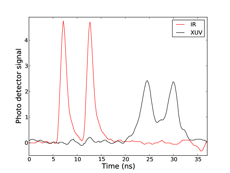
Figure 7: (color online) A typical example of the measured IR-pulse photo-detector signals (red) together with the corresponding XUV-yield at the $15^{th}$ harmonic (black).

The simultaneously measured XUV energy is used as a relative gauge for the density of ions in the HHG interaction zone, as no direct measurement of the level of ionization of the HHG medium was available for the helium measurements. If the phase matching conditions are not severely altered due to ionization, a quadratic dependence of the XUV output on krypton density is expected, while the plasma density, and therefore the phase shift, should be proportional to the density of krypton atoms. We assume that the induced plasma density is proportional to the krypton density, and that no recombination takes place on a timescale of 10 ns.

The relation between XUV yield and ion density was verified in a separate experiment by determining the amount of ionization in the HHG process using a collector grid just below the krypton jet. The voltage applied to this grid was on the order of a few volts to avoid secondary emission. For the conditions in the experiment the relation between XUV energy and recorded number of ions is equal to a power law with an exponent of $2.1(6)$, in good agreement with the expected $2.0$.

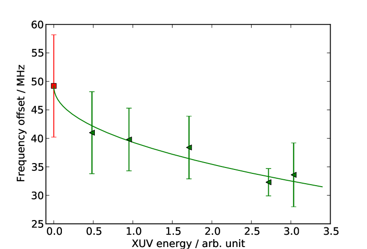
Figure 8: A typical measurement of the frequency offset $f_{ex}$ (the experimental transition frequency relative to the theoretical reference value) as a function of the XUV energy. The XUV energy was varied by changing the gas density in the HHG jet. The green curve is the fitted dependence, while the red square indicates $f_{ex}$ for zero gas density in HHG.

To obtain the ’ionization free’ frequency we extrapolate the frequency offset vs. XUV energy (when varying Kr density) to zero XUV energy using this experimentally determined exponent (see Fig. 8). From the extrapolations we typically find shifts between $0$ and $2$ rad at the $15^{th}$ harmonic for standard conditions, with uncertainties in the range between $0.5$ and $2.0$ rad. The average correction is on the order of $0.1$ XUV cycles. Figure 8 shows the fitting of a typical ionization measurement series, from which a value is derived for $f_{ex}$ at zero gas density in the HHG jet and therefore at zero XUV intensity.

We also have considered krypton atoms in the HHG medium possibly left in an excited state after the first pulse. These excited state atoms would have a different nonlinear susceptibility and therefore produce a different nonlinear phase shift. Such a shift would not be detected by reducing the gas density. However, the HHG cutoff energy for such excited state atoms would lie far below the cutoff energy of the ground state atoms, as the first excited state is about $10$ eV above the ground state. Because the cutoff is already set to the $15^{th}$ harmonic for ground state krypton, this radiation can not be produced by the excited Kr atoms.

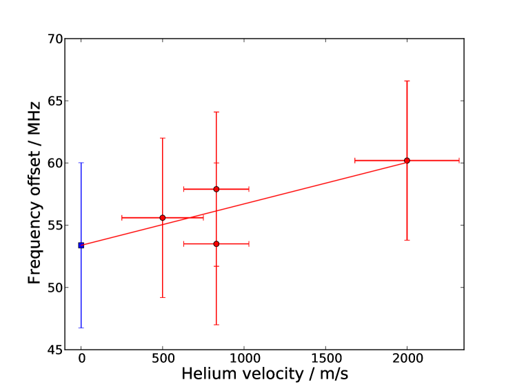
Figure 9: A typical measurement of the frequency offset $f_{ex}$ with respect to the velocity of the helium atoms in the beam. The red line is the fitted dependence, the blue square is the extrapolated Doppler-shift free frequency for zero helium velocity.

The Doppler effect is monitored by varying the helium-beam velocity using mixtures with noble gases. The velocity of helium in the atomic beam is measured (in a separate experiment) by monitoring the frequency shift in the helium signal for different angles between atomic and XUV beam. Helium atoms in the pulsed atomic beam have a speed of $2000(320)$ m/s for a pure-helium expansion, helium in neon (pressure ratio 1:5) results in a speed of $830(200)$ m/s, and helium in argon (pressure ratio 1:5) is slowed down to $500(250)$ m/s). The XUV and atomic beam can be aligned perpendicularly using the different gas mixtures within approximately $10^{-4}$ rad, resulting in a typical statistical error of $13$ MHz for a single Doppler shift determination. Figure 9 shows a typical series, measured with pure helium and the two noble-gas mixtures. A systematic error in the Doppler shift is introduced by the uncertainty in the atomic beam velocity for the different gas mixtures. Because errors in the He velocity lead to a systematic error in the Doppler correction that is proportional to $\cos\phi$ ($\phi$ being the XUV-atomic beam angle) and the angle is kept small with changing signs by readjusting it, the systematic Doppler shift in the ground state energy is smaller than $0.5$ MHz, which is included in the error budget.

V.1.3 Measurement session level errors

The biggest correction at the measurement session level comes from the recoil shift on the considered transitions and can be calculated with high precision. It amounts to $18.28$ and $18.75$ MHz for the $1s$ ${}^{1}\mathrm{S}_{1}-np$ ${}^{1}\mathrm{P}_{1}(n\in 4,5)$ transitions respectively.

As discussed in section III.4, the IR beam is separated from the XUV beam an iris placed after the HHG interaction zone. However, some diffracted IR light can still reach the spectroscopy zone. Compared to the original IR beam, the diffracted light is found to be at least 27 times lower in intensity. this light can still produce an AC-Stark shift but only during the time of the excitation pulses (and not in between), Therefore it shows up in our measurement as a phase shift, which results in a different frequency shift for different $f_{rep}$.

The required correction is determined from a measurement with the beam block removed (i.e. with full IR intensity present in the interaction region). In this case we find a shift of $17.5(6.0)$ MHz on the $1s^{2}$ ${}^{1}\mathrm{S}_{0}-1s5p$ ${}^{1}\mathrm{P}_{1}$ at $148$ MHz repetition frequency. With the beam block inserted for the regular helium measurements, a shift of less then $0.65$ MHz is expected. Converting this to an equivalent phase shift of $14(14)$ mrad in the XUV allows to correct the other measurements performed at different repetition rates.

We have also estimated the theoretically expected frequency shift at $f_{rep}=148$ MHz for the same case. The estimated average peak intensity with the beam stop removed is about $25$ GW/cm², over a pulse duration of $300$ fs. Between the two pulses the intensity is zero. The AC-Stark shift can be calculated by taking the time-averaged intensity Fendel et al. (2007) (for pulses $6.7$ ns apart) of $1$ MW/cm². It leads to a theoretical AC-Stark shift of $20$ MHz, in good agreement with the experimental value, measured with the full IR beam passing the interaction zone.

Finally, we need to consider that the pulses for the phase measurement are split off via a $1$ mm thick beam splitter (with fused silica as substrate material). After this point the pulses travel through the focusing lens (few mm BK7 glass) and enter the vacuum setup for HHG via a Brewster window (another few mm BK7). Any difference in intensity between the two subsequent pulses that are used for the XUV comb generation, or any transient effect in these glass pieces, can cause an additional phase shift which is not taken into account by the generic phase-measurement procedure during recordings of the helium transition. To be able to still correct for this phase shift, a separate experiment was performed removing the IR/XUV separation iris in the vacuum setup. In this way the IR pulses could travel through the interaction zone to the monochromator, where they were coupled out through a window. Two beam splitters inside the monochromator vacuum chamber reduced the pulse energy to less than $0.1\%$ of the original energy, thus avoiding spurious phase effects in the output window and other optics. A phase measurement was then performed on these pulses, while varying the pulse-energy ratio (which can be adjusted via the pump laser). This measurement resulted in an additional correction and uncertainty due to the optics placed between the phase-measurement setup and HHG (beam splitter, lens and Brewster window) of $8.5(15)$ mrad in the IR. This contribution (multiplied by 15 to take the harmonic order into account) is called “NL-phase shift” in the error budget in Table 1, where NL stands for the nonlinear origin of these differential phase shifts.

From Table 1 it is clear that the error contributions differ between the sessions due to different sizes of the corresponding data sets. Also a higher accuracy is achieved for the lower repetition rates in part because phase errors there result in smaller frequency errors. The highest uncertainty of $25$ MHz at $f_{rep}=185$ MHz is based on a very short measurement session, consisting of only one set of Doppler and ’ionization’ series.

V.1.4 Evaluation of the He ground state energy

In the evaluation of the error in the ground state energy, the combined statistical and systematic error based on all sessions ($3.7$ MHz) is combined with several systematic errors represented as frequencies.

The biggest contribution to the uncertainty comes from the ionization shift model. This error contribution listed under “Ionization shift model” in Table 1 refers to the error introduced by the uncertainty in the power law of $2.1(6)$ between the XUV intensity and the amount of ionization (and therefore phase shift) in the harmonic generation region. As this power law is used to correct for the ionization-induced shifts for all measurements at the measurement series level, it results in a systematic error. This is determined by re-analyzing the helium ionization potential for a power law of $1.5$ and $2.7$, resulting in a variation of $4.9$ MHz. As an additional test of (mostly) ionization-induced errors, we also determined the ground state energy using only data points selected within a limited range of XUV-pulse energy, relative to the average XUV energy for each scan. Tests were performed for symmetric and anti-symmetric XUV energy distributions with $5\%$ and $15\%$ deviation from the average XUV energy. A maximum deviation of $5$ MHz (from the value based on all points) was obtained in case of an asymmetric selection of data points with an XUV energy higher than $1.15$ times the average energy. This is comparable with the estimated accuracy of the ionization model as it is based on a typical XUV yield and full distribution of XUV energies.

During the excitation time interval, the extraction fields for the time-of-flight spectrometer are switched off. The estimated residual field of less than $0.5$ V/cm results in a calculated DC-Stark shift on the $5p$, $m=0$ state of less than $20$ kHz. There can be an additional field due to ions in the interaction zone left from the first excitation pulse. However, even for $1000$ ions these fields are too small to cause a significant shift.

The influence of the Zeeman effect is estimated based on the magnetic field measured in the interaction region of $5\times 10^{-5}$ T. Because the excitation radiation originates from HHG, which has essentially zero yield for circular polarization, we can assume the circular component to be less than $1\%$. Since the ground state has no angular momentum, optical pumping cannot occur. Therefore only a weak ($1\%$) $\Delta m=\pm 1$ component has to be taken into account, leading to a Zeeman shift of less than $7$ kHz.

It is vital for Ramsey excitation, that only one transition is excited at a time. Excitation of other states would contribute also with a cosine of almost the same period, but a different phase (which changes quickly with the repetition rate of the FCL). A contribution from the $1s^{2}-1s2p$ transition, which is in the vicinity of the $13^{th}$-harmonic can be excluded, as it can not be ionized with a single $1064$ nm photon. But for the excitation of the $5p$ also the $6p$ level could possibly be excited.

To investigate this, the bandwidth of the XUV pulses was determined by coarse tuning of the IR central wavelength by moving the slit in the Fourier plane of the pulse stretcher, located before the parametric amplifier. As a result, the XUV comb spectrum is tuned as well, and scanned over the transitions. From the signal we subtracted a constant background signal from direct ionization due the $17^{th}$ and higher harmonics. This background has been found by blocking the ionization beam. A typical scan (corrected for the background) is depicted in Fig. 10. The solid line is a Gaussian fit of both the $5p$ and the $6p$ resonance, yielding a 1/e half width of the XUV spectrum of $0.07$ nm at the $15^{th}$ harmonic.

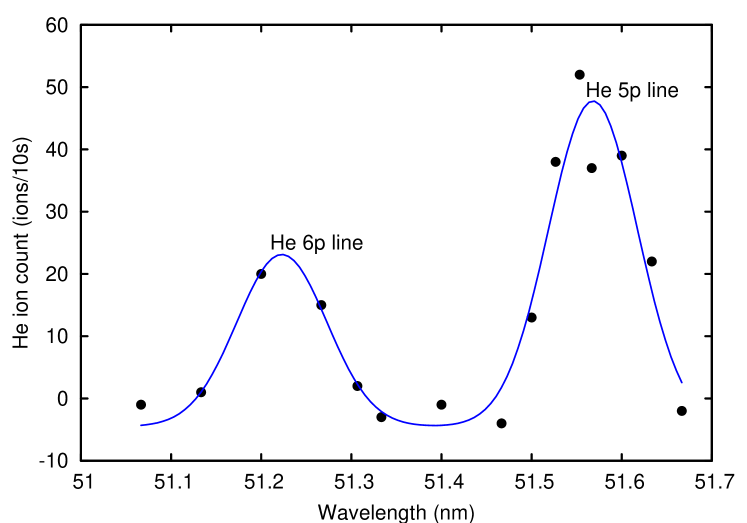
Figure 10: Excitation spectrum (single pulse) from the ground state to the $1s5p$ ${}^{1}\mathrm{P}_{1}$ and $1s6p$ ${}^{1}\mathrm{P}_{1}$ levels in helium, obtained by course scanning of the central wavelength of the fundamental and therefore its $15^{th}$ harmonic over the transitions.

From this width and the Gaussian profile we conservatively estimate a contribution to the $5p$ signal from the $6p$ resonance of less than $1\%$. This can cause a shift of the Ramsey pattern of at most $10$ mrad (in the XUV). However, in practice the influence of this shift on the final transition frequency averages down for different repetition frequencies, so that the maximum error due to excitation of the $6p$ is less than $30$ kHz for all measurements combined.

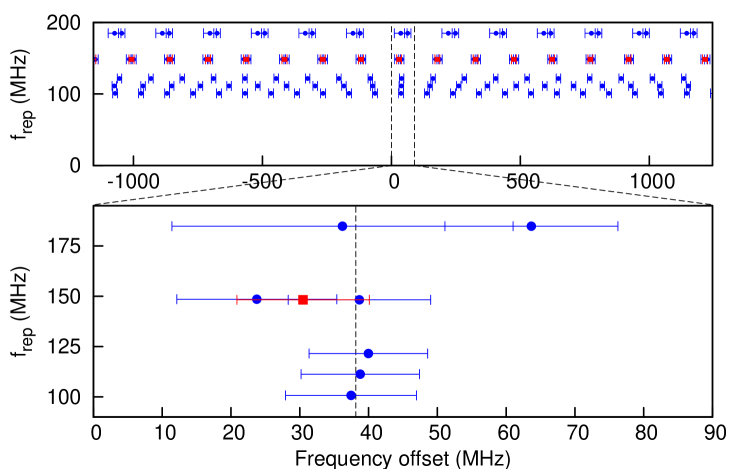
Figure 11: Measured ⁴He ground state binding energy ($\pm nf_{rep}$ ) relative to the theoretical value of $5945204174$ MHz Yerokhin and Pachucki (2010), plotted against the repetition frequency $f_{rep}$ of the comb laser. A clear coincidence is seen at $+37(6)$ MHz relative to theory. The values indicated with a blue solid circle symbol are based on the $1s^{2}$ ${}^{1}\mathrm{S}_{0}-1s5p$ ${}^{1}\mathrm{P}_{1}$ transition. As a cross check, also a value based on the recorded $1s^{2}$ ${}^{1}\mathrm{S}_{0}-1s4p$ ${}^{1}\mathrm{P}_{1}$ transition is included (red square symbol at $f_{rep}=148$ MHz), resulting in a consistent ground state energy.

After incorporating all the systematic corrections, a clear coincidence can be seen between the results for different repetition rates. A new ground state energy for ⁴He of $5945204212(6)$ MHz is found by taking a weighted average over all measured frequencies at the coincidence location. The two most recent theoretical predictions of $5945204174(36)$ MHz from Yerokhin and Pachucki (2010) and $5945204175(36)$ MHz from Drake and Yan (2008) are in agreement with this value within the combined uncertainty of theory and experiment. (The uncertainty of $36$ MHz in both theoretical values is based on estimated but yet uncalculated higher-order QED contributions.) Remarkably, very good agreement is found with the prediction of Korobov Korobov and Yelkhovsky (2001), who calculates $5945204223(42)$ MHz, employing non-relativistic quantum electrodynamics theory, in which the problematic divergences of QED are canceled at the operator level. However, the uncertainties in the present calculations are too large to decide, which of the theoretical approaches is better suited to calculate the energy structure of few electron atoms.

Compared with the best previous determinations using single nanosecond laser pulses Eikema et al. (1997); Bergeson et al. (1998), our new value is almost an order of magnitude more accurate. Good agreement is found with the value of $5945204215(45)$ MHz from Eikema et al. (1997) (based on the measured transition energy in that paper, but corrected for a $14.6$ MHz recoil shift that was previously not taken into account, and using the most recent $2p$ state ionization energy from Yerokhin and Pachucki (2010)). However, there is a difference of nearly $3\sigma$ with the value of $5945204356(50)$ MHz from Bergeson et al. (1998).

Table 1: The error budget for the measurement of the ground-state binding energy of helium. The corrections and uncertainties are given either in radians or in MHz at the $15^{th}$ harmonic, depending on the type of effect (see text). The NL-phase shift denotes the differential phase shift (multiplied by $15$ to account for its effect at the $15^{th}$ harmonic) induced in the optics after the phase measurement but before the HHG jet (see V.1.3).

Effect	Correction	Systematic uncertainty	Statistical uncertainty
Single recording level
Statistical fit error	—	—	typ. 50–150 mrad
Amplifier phase	$0-2.25$ rad	—	$75-375$ mrad
Combined error single recording		—	typ. $160-360$ mrad
Series level
Doppler shift	$0-10$ MHz	see text	$8-18$ MHz
Ionization shift	$0-2$ rad	see ’ionization shift model’	$0.5-2.0$ rad
Session level
AC-Stark shift	$14$ mrad	$14$ mrad - see text	—
NL - phase shift	$128$ mrad	$225$ mrad	—
Recoil shift 4p	18.28 MHz	$\ll 1$ MHz	—
Recoil shift 5p	18.75 MHz	$\ll 1$ MHz	—
Combined error single session		$9-25$ MHz
Ground state evaluation
Weighted mean of sessions	—	$3.7$ MHz
Ionization shift model	—	$4.9$ MHz	—
Doppler shift	—	$500$ kHz	—
DC-Stark shift	—	$<1$ kHz	—
Adjacent 6p-level	—	$<30$ kHz	—
Zeeman shift	—	$<7$ kHz	—
Total error in ground state energy		$6$ MHz

V.2 Signal contrast and phase stability of HHG

In the previous section phase information of the obtained cosine-shaped signals was used to determine the ground state ionization energy of helium. In the following we use the observed contrast of the same helium signals to investigate the phase stability of the generated XUV frequency comb. The signal visibility (ion signal modulation amplitude divided by the average signal) depends on a combination of effects.

The biggest contributions come from the line width of the observed transition, phase stability of the $15^{th}$ harmonic, Doppler broadening, and the width of the IR-FCL modes. In one extreme case ($f_{rep}=185$ MHz, helium seeded in argon) we find a fringe contrast of $55\%$, while for $f_{rep}=100$ MHz and pure helium the contrast is below $5\%$. In Figure 12 the signal contrast is shown for several experimental conditions.

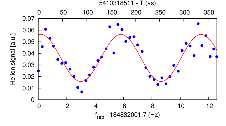
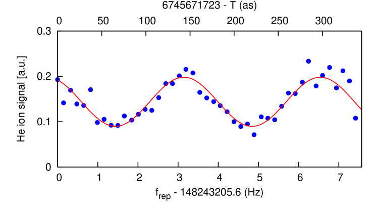
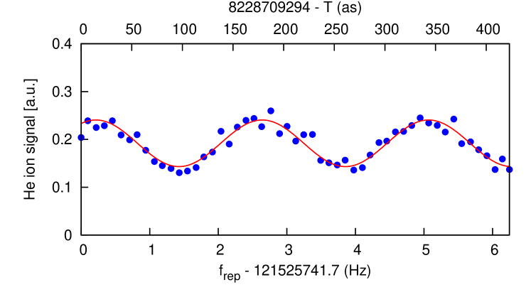
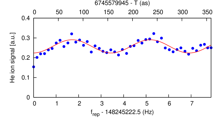
(a) (b) (c) (d)

Figure 12: Ramsey signal of helium, acquired with different experimental conditions. (a) $f_{rep}=185$ MHz, $1s^{2}$ ${}^{1}\mathrm{S}_{0}-1s5p$ ${}^{1}\mathrm{P}_{1}$ transition, helium seeded in argon, contrast: $56\%$, (b) $f_{rep}=148$ MHz, $1s^{2}$ ${}^{1}\mathrm{S}_{0}-1s5p$ ${}^{1}\mathrm{P}_{1}$ transition, helium seeded in neon, contrast: $38\%$, (c) $f_{rep}=121$ MHz, $1s^{2}$ ${}^{1}\mathrm{S}_{0}-1s5p$ ${}^{1}\mathrm{P}_{1}$ transition, helium seeded in neon, contrast: $25\%$, (d) $f_{rep}=148$ MHz, $1s^{2}$ ${}^{1}\mathrm{S}_{0}-1s4p$ ${}^{1}\mathrm{P}_{1}$ transition, pure helium beam, contrast: $13\%$.

From an analysis of the observed visibility of the interference pattern as a function of the helium-beam velocity and comb repetition frequency, an estimate for the XUV comb phase jitter and of the effective width of the angular distribution of the atomic beam can be derived. We model the Ramsey pattern assuming Gaussian phase noise, while the Doppler effect is taken into account with various distributions, including Gaussian and rectangular. Both Doppler and phase-noise distribution widths are fitted in the procedure to the observed visibilities, and scans are included that were used in the frequency determination, plus additional scans that were performed on the $6p$ and $7p$ transitions. In all cases we assume a common background count rate of $15\%$. The resulting Doppler width and phase jitter depends on the function used for the Doppler distribution. For a Gaussian profile, we find a FWHM angular beam divergence of $2.4$ mrad and $0.42$ cycles XUV jitter. A rectangular distribution leads to a divergence angle of $4.3$ mrad and $0.35$ cycles XUV phase jitter. In both cases the model seems to have deficiencies. While in the former case the visibility seems to be systematically underestimated for slow beams, in the latter case this underestimation is less pronounced and the fit becomes worse for the fast He beams where the angular distribution is important. We therefore estimate an intermediate value of $0.38(6)$ cycles for the XUV phase jitter.

If we consider the contributions to the XUV comb jitter then the biggest contribution arises from the bandwidth of the modes of the FC in the IR. The bandwidth of the FC was measured in a separate experiment by beating the FC modes with a frequency doubled narrow bandwidth Er-fiber laser (NP Photonics, with a short-term line width of $5$ kHz) to yield a value of $1.6$ MHz FWHM, corresponding to a jitter of $1/6$ of an XUV cycle.

A second contribution comes from the phase uncertainty of $47$ mrad FWHM in the amplified pulses after correction for the measured phase shift (evaluated near the peak intensity of the pulse), leading to a jitter of $1/9$ cycle in the XUV. For HHG we take into account that the phase of the generated harmonics is proportional to the intensity of the fundamental beam Lewenstein et al. (1994), with an estimated factor of $\approx 10^{-13}$ rad cm²/ W, using the results presented in Corsi et al. (2006). Combined with an NOPCPA pulse-ratio distribution FWHM of $2.5\%$, this gives a small expected jitter of $0.02$ XUV cycles. Fluctuations of $6\%$ in the IR pulse intensity lead to variations in the level of ionization in the HHG jet of more than $35\%$ (as ionization scales with at least the $7^{th}$ power of the IR intensity for the conditions in the experiment). If we adopt a typical average ionization correction of $0.1$ XUV cycles, then this induces a phase jitter of $0.04$ XUV cycles. Krypton density fluctuations ($<20\%$) induce less than half this value.

Statistically independent combination of these noise sources leads to a total expected phase jitter in the XUV of $0.21$ cycles. This is lower, but comparable to the jitter extracted from the contrast measurements. The difference might be due to uncertainties in the exact experimental conditions, in particular the Doppler broadening and the bandwidth of the frequency comb laser modes during the experiments.

The (estimated) contributions to the jitter suggest that the contrast should hardly be influenced by intensity-induced phase noise from the HHG process. This was investigated experimentally by taking only a subset of the data points to determine the contrast, using a selection criterion based on the measured XUV intensity. With this procedure we find that the visibility of the interference does not change (within a few percent) if we restrict the XUV intensity variation to symmetric bands of $5\%$, and $40\%$ around the mean XUV energy. We therefore conclude that intensity dependent effects do not play a significant role as a source of phase noise in the XUV comb in the present experiment.

VI Conclusions and outlook

The metrology presented in this article represents a significant advance in the history of precision extreme ultraviolet spectroscopy. As is illustrated in the historical overview of the spectroscopy of the helium atom, depicted in Fig. 13, the theoretical and experimental accuracy of the value of the binding energy of helium improved by many orders of magnitude over the last hundred years. Experimentally the biggest progress has always been initiated by new methods, which in turn also lead to advances in the theoretical understanding. The pioneering measurement by Herzberg Herzberg (1958) in 1958 based on a helium lamp and grating spectrometer was not significantly improved upon until the first laser excitation in 1993 Eikema et al. (1993).

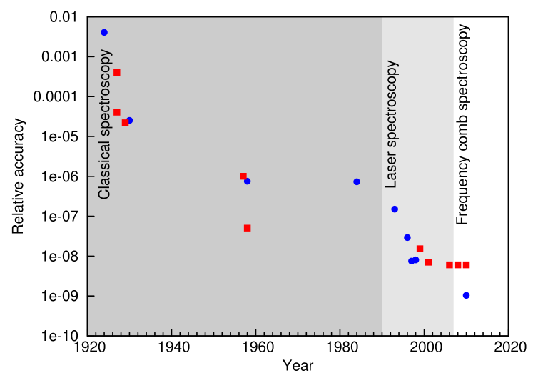
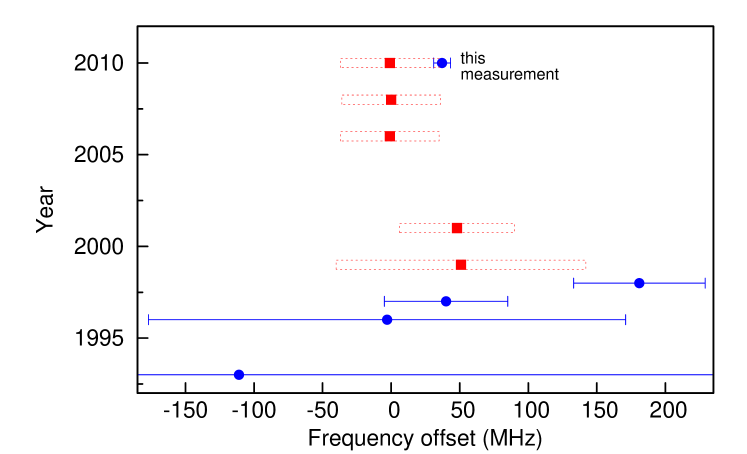
(a) (b)

Figure 13: (color online) (a) Advance in theoretical and spectroscopic accuracy of the ground state energy of helium over the last 100 years. The shaded areas emphasize new spectroscopic tools that allowed to overcome limits of previous technologies. Red squares represent the precision of calculations. The precision obtained in experiments is indicated with blue circles. (b) Comparison of helium ground state ionization energy values obtained experimentally (blue circles) and theoretically (red squares) in the last two decades. The values are plotted with respect to the most recent theoretical result Bergeson et al. (1998); Eikema et al. (1997); Herzberg (1958); Hylleraas (1929); Kabir and Salpeter (1957); Hopfield (1930); Kellner (1927); Slater (1927); Yerokhin and Pachucki (2010); Baig et al. (1984); Drake (1999); Drake and Yan (2008); Eikema et al. (1993, 1996); Korobov and Yelkhovsky (2001); Lyman (1924); Pachucki (2006); Sucher (1958).

In this paper we have described the first absolute frequency measurement in the XUV spectral region, based on parametric amplification and harmonic upconversion of two pulses from an IR frequency comb laser. Direct frequency comb excitation in the XUV of helium from the ground state is demonstrated, leading to an almost 10-fold improved ground state ionization energy, and in good agreement with theory.

For the employed method it is vitally important to control and detect phase shifts in the amplification and harmonic upconversion process. An important aspect of direct excitation with an upconverted frequency comb is the possibility to detect systematic errors due to phase shifts between the pulses from the NOPCPA, HHG and ionization, but also from the AC-Stark effect. Uncorrected errors of this kind show up as a frequency shift that is proportional to $f_{rep}$, and can therefore be detected easily. In the current experiment no dependence on the repetition rate is observed in the measurements (see Fig. 11), indicating that the systematic effects have been taken into account properly. The accuracy of the presented method scales with $f_{rep}$, which also means that it can be improved by orders of magnitude by choosing frequency comb pulses further apart. If the pulse delay would be extended to $>150$ ns, then the ionization shift introduced in the HHG process would in fact vanish altogether, as the time between the pulses would be sufficiently long to replace the gas in the focal region with a new sample before the second pulse arrives. This would reduce the error in the spectroscopy significantly because the biggest source of uncertainty is currently due to ionization effects in the HHG process. To fully exploit the enhanced accuracy with larger pulse delays, the sample has to be trapped and cooled to reduce Doppler and time-of-flight broadening which would otherwise wash out the ever denser signal modulation. In view of this, measurements on He⁺ are particularly interesting. This ion has a hydrogen-like electronic configuration which can be excited from the ground state using a two-photon transition at $60$ nm. Such an experiment has the potential to perform QED tests beyond what has been possible so far in atomic hydrogen Fischer et al. (2004); Herrmann et al. (2009).

In the present work a frequency comb laser in the XUV range is demonstrated, for the first time at wavelengths as short as $51$ nm. The phase jitter of the XUV frequency comb modes is found to be $0.38(6)$ cycles. From the results we conclude that the observed comb jitter in the XUV is not dominated by the HHG upconversion process, but most likely by the stability of the original comb in the infrared. This form of technical noise can be considerably reduced by locking the comb laser to a stable optical reference cavity. It seems therefore feasible to extend comb generation and spectroscopy to even shorter wavelengths into the soft-X-ray region, provided that the carrier-phase noise of the fundamental and upconverted pulses is kept low enough. Further possibilities would arise if not subsequent pulses from the FC, but any two-pulse sequence could be selected for upconversion. This would increase the accuracy significantly below 1 MHz as the pulses could have a much increased time delay, thus making it possible to resolve multiple transitions with discrete Fourier transform spectroscopy techniques. In view of these possibilities, we envision applications such as QED test of He⁺ and highly charged ions, precision spectroscopy of simple molecules such as $\mathrm{H}_{2}$, coherent XUV or X-ray imaging, and possibly even the emergence of X-ray nuclear clocks.

References

- Lamb and Retherford (1947) W. E. Lamb and R. C. Retherford, Phys. Rev., 72, 241 (1947).
- Lamb and Retherford (1950) W. E. Lamb and R. C. Retherford, Phys. Rev., 79, 549 (1950).
- Feynman (1949) R. P. Feynman, Phys. Rev., 76, 769 (1949).
- Schwinger (1948) J. Schwinger, Phys. Rev., 74, 1439 (1948).
- Tomonaga (1946) S. Tomonaga, Prog. Theor. Phys., 1, 27 (1946).
- Huber et al. (1999) A. Huber, B. Gross, M. Weitz, and T. W. Hänsch, Phys. Rev. A, 59, 1844 (1999).
- Parthey et al. (2010) C. G. Parthey, A. Matveev, J. Alnis, R. Pohl, T. Udem, U. D. Jentschura, N. Kolachevsky, and T. W. Hänsch, Phys. Rev. Lett., 104, 233001 (2010).
- Gumberidze et al. (2005) A. Gumberidze, T. Stohlker, D. Banas, K. Beckert, P. Beller, H. F. Beyer, F. Bosch, S. Hagmann, C. Kozhuharov, D. Liesen, F. Nolden, X. Ma, P. H. Mokler, M. Steck, D. Sierpowski, and S. Tashenov, Phys. Rev. Lett., 94, 223001 (2005).
- Hagena et al. (1993) D. Hagena, R. Ley, D. Weil, G. Werth, W. Arnold, and H. Schneider, Phys. Rev. Lett., 71, 2887 (1993).
- Meyer et al. (2000) V. Meyer, S. N. Bagayev, P. E. G. Baird, P. Bakule, M. G. Boshier, A. Breitrück, S. L. Cornish, S. Dychkov, G. H. Eaton, A. Grossmann, D. Hübl, V. W. Hughes, K. Jungmann, I. C. Lane, Y.-W. Liu, D. Lucas, Y. Matyugin, J. Merkel, G. zu Putlitz, I. Reinhard, P. G. H. Sandars, R. Santra, P. V. Schmidt, C. A. Scott, W. T. Toner, M. Towrie, K. Träger, L. Willmann, and V. Yakhontov, Phys. Rev. Lett., 84, 1136 (2000).
- Korobov et al. (2009) V. I. Korobov, L. Hilico, and J.-P. Karr, Phys. Rev. A, 79, 012501 (2009).
- Koelemeij et al. (2007) J. C. J. Koelemeij, B. Roth, A. Wicht, I. Ernsting, and S. Schiller, Phys. Rev. Lett., 98, 173002 (2007).
- Salumbides et al. (2011) E. J. Salumbides, G. D. Dickenson, T. I. Ivanov, and W. Ubachs, Phys. Rev. Lett., 107, 043005 (2011).
- Hanneke et al. (2008) D. Hanneke, S. Fogwell, and G. Gabrielse, Phys. Rev. Lett., 100, 120801 (2008).
- Fischer et al. (2004) M. Fischer, N. Kolachevsky, M. Zimmermann, R. Holzwarth, Th. Udem, T. W. Hänsch, M. Abgrall, J. Grünert, I. Maksimovic, S. Bize, H. Marion, F. Pereira Dos Santos, P. Lemonde, G. Santarelli, P. Laurent, A. Clairon, C. Salomon, M. Haas, U. Jentschura, and C. Keitel, Phys. Rev. Lett., 92, 230802 (2004).
- Pachucki and Jentschura (2003) K. Pachucki and U. D. Jentschura, Phys. Rev. Lett., 91, 113005 (2003).
- Pohl et al. (2010) R. Pohl, A. Antognini, F. Nez, F. D. Amaro, F. Biraben, J. M. R. Cardoso, D. S. Covita, A. Dax, S. Dhawan, L. M. P. Fernandes, A. Giesen, T. Graf, T. W. Hansch, P. Indelicato, L. Julien, C. Y. Kao, P. Knowles, E. O. Le Bigot, Y. W. Liu, J. A. M. Lopes, L. Ludhova, C. M. B. Monteiro, F. Mulhauser, T. Nebel, P. Rabinowitz, J. M. F. dos Santos, L. A. Schaller, K. Schuhmann, C. Schwob, D. Taqqu, J. F. C. A. Veloso, and F. Kottmann, Nature, 466, 213 (2010).
- Jentschura (2011) U. D. Jentschura, Eur. Phys. J. D., 61, 7 (2011).
- De Rujula (2011) A. De Rujula, Phys. Lett. B, 697, 26 (2011).
- Cloet and Miller (2011) I. C. Cloet and G. A. Miller, Phys. Rev. C, 83, 012201 (2011).
- Barger et al. (2011) V. Barger, C. W. Chiang, W. Y. Keung, and D. Marfatia, Phys. Rev. Lett., 106, 153001 (2011).
- Epp et al. (2010) S. W. Epp, J. R. C. Lopez-Urrutia, M. C. Simon, T. Baumann, G. Brenner, R. Ginzel, N. Guerassimova, V. Mackel, P. H. Mokler, B. L. Schmitt, H. Tawara, and J. Ullrich, J. Phys. B - At. Mol. Opt., 43, 194008 (2010).
- Eikema et al. (1993) K. Eikema, W. Ubachs, W. Vassen, and W. Hogervorst, Phys. Rev. Lett., 71, 1690 (1993).
- Eikema et al. (1997) K. S. E. Eikema, W. Ubachs, W. Vassen, and W. Hogervorst, Phys. Rev. A, 55, 1866 (1997).
- Eikema et al. (1996) K. S. E. Eikema, W. Ubachs, W. Vassen, and W. Hogervorst, Phys. Rev. Lett., 76, 1216 (1996).
- Bergeson et al. (1998) S. D. Bergeson, A. Balakrishnan, K. G. H. Baldwin, T. B. Lucatorto, J. P. Marangos, T. J. McIlrath, T. R. O’Brian, S. L. Rolston, C. J. Sansonetti, J. Wen, N. Westbrook, C. H. Cheng, and E. E. Eyler, Phys. Rev. Lett., 80, 3475 (1998).
- Bergeson et al. (2000) S. D. Bergeson, K. G. H. Baldwin, T. B. Lucatorto, T. J. McIlrath, C. H. Cheng, and E. E. Eyler, J. Opt. Soc. Am. B, 17, 1599 (2000).
- Ramsey (1949) N. F. Ramsey, Phys. Rev., 76, 996 (1949).
- Salour and Cohen-Tannoudji (1977) M. M. Salour and C. Cohen-Tannoudji, Phys. Rev. Lett., 38, 757 (1977).
- Teets et al. (1977) R. Teets, J. Eckstein, and T. W. Hänsch, Phys. Rev. Lett., 38, 760 (1977).
- Eckstein et al. (1978) J. Eckstein, A. I. Ferguson, and T. W. Hänsch, Phys. Rev. Lett., 40, 847 (1978).
- Salieres et al. (1999) P. Salieres, L. Le Deroff, T. Auguste, P. Monot, P. d’Oliveira, D. Campo, J. F. Hergott, H. Merdji, and B. Carre, Phys. Rev. Lett., 83, 5483 (1999).
- Bellini et al. (2001) M. Bellini, S. Cavalieri, C. Corsi, and M. Materazzi, Opt. Lett., 26, 1010 (2001).
- Kovačev et al. (2005) M. Kovačev, S. V. Fomichev, E. Priori, Y. Mairesse, H. Merdji, P. Monchicourt, P. Breger, J. Norin, A. Persson, A. L’Huillier, C.-G. Wahlström, B. Carré, and P. Salières, Phys. Rev. Lett., 95, 223903 (2005).
- Liontos et al. (2010) I. Liontos, S. Cavalieri, C. Corsi, R. Eramo, S. Kaziannis, A. Pirri, E. Sali, and M. Bellini, Opt. Lett., 35, 832 (2010).
- Diddams et al. (2000) S. A. Diddams, D. J. Jones, J. Ye, S. T. Cundiff, J. L. Hall, J. K. Ranka, R. S. Windeler, R. Holzwarth, Th. Udem, and T. W. Hänsch, Phys. Rev. Lett., 84, 5102 (2000).
- Holzwarth et al. (2000) R. Holzwarth, Th. Udem, T. W. Hänsch, J. C. Knight, W. J. Wadsworth, and P. St. J. Russel, Phys. Revi. Lett., 85, 2264 (2000).
- Seres et al. (2005) J. Seres, E. Seres, A. J. Verhoef, G. Tempea, C. Strelill, P. Wobrauschek, V. Yakovlev, A. Scrinzi, C. Spielmann, and F. Krausz, Nature, 433, 596 (2005).
- Fendel et al. (2007) P. Fendel, S. D. Bergeson, Th. Udem, and T. W. Hänsch, Opt. Lett., 32, 701 (2007).
- Marian et al. (2005) A. Marian, M. C. Stowe, D. Felinto, and J. Ye, Phys. Rev. Lett., 95, 023001 (2005).
- Wolf et al. (2009) A. L. Wolf, S. A. van den Berg, W. Ubachs, and K. S. E. Eikema, Phys. Rev. Lett., 102, 223901 (2009).
- Witte et al. (2005) S. Witte, R. Th. Zinkstok, W. Ubachs, W. Hogervorst, and K. S. E. Eikema, Science, 307, 400 (2005).
- Zinkstok et al. (2006) R. Th. Zinkstok, S. Witte, W. Ubachs, W. Hogervorst, and K. S. E. Eikema, Phys. Rev. A, 73, 061801 (2006).
- Lewenstein et al. (1994) M. Lewenstein, Ph. Balcou, M. Yu. Ivanov, A. L’Huillier, and P. B. Corkum, Phys. Rev. A, 49, 2117 (1994).
- Cavalieri et al. (2002) S. Cavalieri, R. Eramo, M. Materazzi, C. Corsi, and M. Bellini, Phys. Rev. Lett., 89, 133002 (2002).
- Zerne et al. (1997) R. Zerne, C. Altucci, M. Bellini, M. B. Gaarde, T. W. Hänsch, A. L’Huillier, C. Lyngå, and C. G. Wahlström, Phys. Rev. Lett., 79, 1006 (1997).
- Gohle et al. (2005) Ch. Gohle, Th. Udem, M. Herrmann, J. Rauschenberger, R. Holzwarth, H. A. Schuessler, F. Krausz, and T. W. Hänsch, Nature, 436, 234 (2005).
- Jones et al. (2005) R. J. Jones, K. D. Moll, M. J. Thorpe, and J. Ye, Phys. Rev. Lett., 94, 193201 (2005).
- Ozawa et al. (2008) A. Ozawa, J. Rauschenberger, Ch. Gohle, M. Herrmann, D. R. Walker, V. Pervak, A. Fernandez, R. Graf, A. Apolonski, R. Holzwarth, F. Krausz, T. W. Hänsch, and Th. Udem, Phys. Rev. Lett., 100, 253901 (2008).
- Yost et al. (2009) D. C. Yost, T. R. Schibli, J. Ye, J. L. Tate, J. Hostetter, M. B. Gaarde, and K. J. Schafer, Nat. Phys., 5, 815 (2009).
- Kandula et al. (2010) D. Z. Kandula, C. Gohle, T. J. Pinkert, W. Ubachs, and K. S. E. Eikema, Phys. Rev. Lett., 105, 063001 (2010).
- Kandula et al. (2008) D. Z. Kandula, A. Renault, Ch. Gohle, A. L. Wolf, S. Witte, W. Hogervorst, W. Ubachs, and K. S. E. Eikema, Opt. Express, 16, 7071 (2008).
- Lewenstein et al. (1995) M. Lewenstein, P. Salières, and A. L’Huillier, Phys. Rev. A, 52, 4747 (1995).
- Pirri et al. (2007) A. Pirri, C. Corsi, E. Sali, A. Tortora, and M. Bellini, Laser Phys., 17, 138 (2007).
- Witte et al. (2006) S. Witte, R. Th. Zinkstok, A. L. Wolf, W. Hogervorst, W. Ubachs, and K. S. E. Eikema, Opt. Express, 14, 8168 (2006).
- Renault et al. (2007) A. Renault, D. Z. Kandula, S. Witte, A. L. Wolf, R. Th. Zinkstok, W. Hogervorst, and K. S. E. Eikema, Opt. Lett., 32, 2363 (2007).
- Ross et al. (2002) I. N. Ross, P. Matousek, G. H. C. New, and K. Osvay, J. Opt. Soc. Am. B, 19, 2945 (2002).
- Witte et al. (2007) S. Witte, R. Th. Zinkstok, W. Hogervorst, and K. S. E. Eikema, Appl. Phys. B, 87, 677 (2007).
- Press et al. (1992) W. H. Press, S. A. Teukolsky, W. T. Vetterling, and B. P. Flannery, Numerical Recipes in C: the Art of Scientific Computing (Cambridge University Press, 1992) p. 1235.
- Yerokhin and Pachucki (2010) V. A. Yerokhin and K. Pachucki, Phys. Rev. A, 81, 022507 (2010).
- Morton et al. (2006) D. C. Morton, Q. Wu, and G. W. F. Drake, Can. J. Phys., 84, 83 (2006).
- Drake and Yan (2008) G. W. F. Drake and Z. C. Yan, Can. J. Phys., 86, 45 (2008).
- Korobov and Yelkhovsky (2001) V. Korobov and A. Yelkhovsky, Phys. Rev. Lett., 87, 193003 (2001).
- Corsi et al. (2006) C. Corsi, A. Pirri, E. Sali, A. Tortora, and M. Bellini, Phys. Rev. Lett., 97, 023901 (2006).
- Herzberg (1958) G. Herzberg, P. R. Soc. Lond. A - Conta., 248, 309 (1958).
- Hylleraas (1929) E. A. Hylleraas, Z. Phys., 54, 347 (1929).
- Kabir and Salpeter (1957) P. K. Kabir and E. E. Salpeter, Phys. Rev., 108, 1256 (1957).
- Hopfield (1930) J. J. Hopfield, Astrophys. J., 72, 133 (1930).
- Kellner (1927) G. W. Kellner, Z. Phys., 44, 91 (1927).
- Slater (1927) J. C. Slater, P. Natl. Acad. Sci. USA, 13, 423 (1927).
- Baig et al. (1984) M. A. Baig, J. P. Connerade, C. Mayhew, G. Noeldeke, and M. J. Seaton, J. Phys. B- At. Mol. Opt., 17, L383 (1984).
- Drake (1999) G. W. F. Drake, Phys. Scripta, 1999, 83 (1999).
- Lyman (1924) T. Lyman, Astrophys. J., 60, 1 (1924).
- Pachucki (2006) K. Pachucki, Phys. Rev. A, 74, 022512 (2006).
- Sucher (1958) J. Sucher, Phys. Rev., 109, 1010 (1958).
- Herrmann et al. (2009) M. Herrmann, M. Haas, U. D. Jentschura, F. Kottmann, D. Leibfried, G. Saathoff, C. Gohle, A. Ozawa, V. Batteiger, S. Knünz, N. Kolachevsky, H. A. Schüssler, T. W. Hänsch, and Th. Udem, Phys. Rev. A, 79, 052505 (2009).