Nonholonomic LL systems on central extensions and
the hydrodynamic Chaplygin sleigh with circulation

Abstract

We consider nonholonomic systems whose configuration space is the central extension of a Lie group and have left invariant kinetic energy and constraints. We study the structure of the associated Euler-Poincaré-Suslov equations and show that there is a one-to-one correspondence between invariant measures on the original group and on the extended group. Our results are applied to the hydrodynamic Chaplygin sleigh, that is, a planar rigid body that moves in a potential flow subject to a nonholonomic constraint modeling a fin or keel attached to the body, in the case where there is circulation around the body.

1 Introduction and outline

In this paper, we study the equations of motion for mechanical systems on central extension type Lie groups with nonholonomic constraints, where both the constraints and the kinetic energy are invariant under the left action of the group on itself. Our main motivating example comes from hydrodynamics and consists of a nonholonomic sleigh immersed in a two-dimensional potential flow with circulation.

The Euler-Poincaré-Suslov equations.

An LL system is a mechanical system on a Lie group $G$ with a kinetic energy Lagrangian and a set of nonholonomic constraints, so that both the Lagrangian and the constraints are left-invariant under the action of $G$ on itself. Due to the invariance under the group action, the dynamics reduce to the Lie algebra $\mathfrak{g}$, or to its dual $\mathfrak{g}^{*}$ if working with the momentum formulation. The resulting reduced equations are termed the Euler-Poincaré-Suslov (EPS) equations [8].

In this paper, we consider EPS equations associated to nonholonomic LL systems for which the underlying Lie group is a central extension. We apply the criterion of Jovanović [10] (see also [14]) to obtain necessary and sufficient conditions on the existence of invariant measures for these equations. One of our theoretical results is Theorem 3.1, which states that an EPS system on a central extension $\widehat{G}$ has an invariant measure if and only if the corresponding system on the original Lie group $G$ has an invariant measure.

The hydrodynamic Chaplygin sleigh.

Our motivating example of an EPS system on a central extension is given by the motion of a two-dimensional rigid body which moves inside a potential flow with circulation $\kappa\neq 0$, where the nonholonomic constraint precludes motion transversal to the body, modeling, for instance, a very effective keel or fin.

This model was first considered in the absence of circulation in [6], where it was termed the hydrodynamic Chaplygin sleigh. This terminology reflects the fact that in the absence of the fluid, the nonholonomic constraint models the effect of a sharp blade in the classical Chaplygin sleigh problem [5] which prevents the sleigh from moving in the lateral direction. In the presence of the fluid, the constraint can be interpreted as modeling the effect of a very effective keel or fin on the body [6]. It is an interesting historic coincidence that the name of Chaplygin is linked both to the development of the Chaplygin-Lamb equations [4] as well as to the nonholonomic Chaplygin sleigh [5]. Similar models for two-dimensional swimmers have been studied in [12] (see also [23]). The motion of the hydrodynamic Chaplygin sleigh in the presence of circulation is treated in [7]. However, to the best of our knowledge this is the first time that the geometric nature of the system is elucidated.

The Chaplygin-Lamb equations.

When the effect of the keel is ignored, so that there are no nonholonomic constraints, the equations of motion for the hydrodynamic sleigh reduce to the Chaplygin-Lamb equations [4, 15]. We show that these equations can be viewed in two different, but equivalent ways:

1. As a left-invariant system on the group $\operatorname{SE}(2)$ of translations and rotations in the plane, moving under the influence of a gyroscopic force. The latter is termed the Kutta-Zhukowski force [18] and models the effect of nonvanishing circulation on the body.

2. As a geodesic system on a central extension of $\operatorname{SE}(2)$ by $\mathbb{R}^{3}$ that we denote by $\widehat{G}$, where the extra variables in the $\mathbb{R}^{3}$-factor describe the circulation. In this way, the Kutta-Zhukowski force becomes a geometric effect, which is not added explicitly to the system but appears a posteriori as a consequence of how the central extension is constructed.

A classical counterpart of this duality is the description of a particle of charge $e$ moving under the influence of a magnetic field $B$ perpendicular to the plane of motion. As is well known, such a particle may be modeled either as moving under the influence of the Lorentz force, or as a particle moving in the Heisenberg group $\mathbb{R}^{2}\times\mathbb{S}^{1}$ equipped with a group multiplication involving the magnetic field (see [19]). In the example of the hydrodynamic Chaplygin sleigh, the circulation $\kappa$ plays the role of the charge, and the cocycle will be discussed below.

The nature of the cocycles.

In constructing the extension $\widehat{G}$ of $\operatorname{SE}(2)$ by $\mathbb{R}^{3}$, we introduce an $\mathbb{R}^{3}$-valued two-cocycle $C:\mathfrak{se}(2)\times\mathfrak{se}(2)\to\mathbb{R}^{3}$ which can be decomposed on fluid-dynamical grounds as $C=(C_{1},C_{2})$, where $C_{1}$ takes values in $\mathbb{R}$ while $C_{2}$ is $\mathbb{R}^{2}$-valued. As we have pointed out before, each of these cocycles is responsible for the appearance of certain gyroscopic forces in the equations of motion, and we now discuss these forces some more.

The first cocycle, $C_{1}$, is “essential” in the sense that it cannot be written as the coboundary (defined below) of a one-cocycle $\mathcal{A}$, and we argue that this is a consequence of Kelvin’s theorem, which states that circulation is constant. By contrast, the second cocycle $C_{2}$ is exact, and we show that it can be “gauged away” by adequately choosing the origin of the body reference frame. From a physical point of view, the cocycle $C_{2}$ is associated to the moment generated by the Kutta-Zhukowski force. While it would have been possible to get rid of $C_{2}$, this would complicate the description of the nonholonomic constraint that we discuss below.

Adding nonholonomic constraints.

The effect of the keel gives rise to a nonholonomic constraint on the system, which can be viewed as follows: if we affix a frame $\{\mathbf{E}_{1},\mathbf{E}_{2}\}$ to the body, with $\mathbf{E}_{1}$ aligned with the keel and $\mathbf{E}_{2}$ perpendicular to it, the effect of the keel is to preclude motion in the $\mathbf{E}_{2}$-direction, or in other words

$$v_{2}=0,$$ (1.1)

where $v_{2}$ is the component of the body velocity in the direction of $\mathbf{E}_{2}$. This is a constraint on the velocities which cannot be integrated to give a relation between the admissible configurations of the body, and is therefore nonholonomic. Just as the kinetic energy, this constraint is left invariant under the action of the central extension $\widehat{G}$ on itself, and therefore gives rise to an EPS system on $\widehat{\mathfrak{g}}$, the Lie algebra of $\widehat{G}$.

Using the geometric structure of the equations, we are able to obtain necessary and sufficient conditions for the existence of an invariant measure (Proposition 4.3). Among other things, we show that the existence of an invariant measure is independent of the circulation.

Outline.

The paper is organized as follows. In Section 2 we recall the necessary preliminaries on the theory of central extensions of Lie groups with the viewpoint on their mechanical applications. In Section 3 we consider the EPS equations of LL systems whose underlying Lie group is a central extension and give conditions for the existence of invariant measures in Theorem 3.1.

Section 4 considers the structure of the equations of motion for planar rigid bodies moving on a perfect fluid with circulation. Our contributions are contained in Theorem 4.2 that describes the geometric structure of the most general form of the Chaplygin-Lamb equations and in the construction in subsection 4.3 where we show that the reduced equations for the hydrodynamic Chaplygin sleigh with circulation are of EPS type, and where we give conditions for measure preservation. These results rely on the introduction of the group cocycle that defines a central extension of the group $\operatorname{SE}(2)$ described above, and that is studied in detail in Section 5.

2 Central extensions of Lie groups

We briefly recall the definitions and basic properties of central extensions of Lie groups to introduce the relevant notation. A detailed account of the geometry of central extensions in the context of mechanics can be found in [17, 16, 13].

Definition.

Let $G$ be a Lie group and $A$ an abelian Lie group. We will use additive notation for the group operation in $A$. For our purposes, a central extension of $G$ by $A$ is a Lie group $\widehat{G}$ such that $\widehat{G}=G\times A$ equipped with the group multiplication

$$(g,\alpha)(h,\beta)=(gh,\alpha+\beta+B(g,h)),$$ (2.2)

where $B:G\times G\to A$ is a normalized group two-cocycle. Associativity of the multiplication on $\widehat{G}$ is equivalent to the two-cocycle identity,

$$B(f,g)+B(fg,h)=B(f,gh)+B(g,h)\qquad\mbox{for all}\qquad f,g,h\in G.$$

The assumption that the two-cocycle $B$ is normalized can be made without loss of generality and amounts to

$$B(g,e)=B(e,g)=0\qquad\mbox{for all}\qquad g\in G,$$

implying that $B(g,g^{-1})=B(g^{-1},g)$.

Central extension of Lie algebras.

The Lie algebra $\widehat{\mathfrak{g}}$ of $\widehat{G}$ is isomorphic as a vector space to $\mathfrak{g}\times\mathfrak{a}$, and is equipped with the following bracket:

$$[(\xi,a),(\eta,b)]_{\widehat{\mathfrak{g}}}=([\xi,\eta]_{\mathfrak{g}},C(\xi,\eta))$$

for $(\xi,a),\,(\eta,b)\in\widehat{\mathfrak{g}}$. Here, the $\mathfrak{a}$-valued Lie algebra two-cocycle $C:\mathfrak{g}\times\mathfrak{g}\to\mathfrak{a}$ is defined by

$$C(\xi,\eta):=\left.\frac{\partial^{2}}{\partial s\partial t}\right|_{s=t=0}(B(g(t),h(s))-B(h(s),g(t))),\qquad i=1,2,$$ (2.3)

with $g(t),\,h(s)$ smooth curves on $G$ satisfying $\dot{g}(0)=\xi,\;\dot{h}(0)=\eta$.

It may happen that $C$ can be written in terms of a one-cocycle $\mathcal{A}:\mathfrak{g}\to\mathfrak{a}$ as $C(\xi,\eta)=-\mathcal{A}([\xi,\eta])$ for all $\xi,\eta\in\mathfrak{g}$. In this case, $C$ is a coboundary in the sense of Lie algebra cohomology, and we write $C=\delta\mathcal{A}$. When this happens, the central extension is said to be trivial, as the mapping

$$\Psi_{\mathcal{A}}:\mathfrak{g}\times\mathfrak{a}\to\widehat{\mathfrak{g}},\quad(\xi,a)\mapsto(\xi,a-\mathcal{A}(\xi))$$ (2.4)

then determines a Lie algebra isomorphism between the Lie algebra $\mathfrak{g}\times\mathfrak{a}$ with the product bracket and the central extension $\widehat{\mathfrak{g}}$.

Lie-Poisson structures.

As a vector space, the dual Lie algebra $\widehat{\mathfrak{g}}^{*}$ equals $\mathfrak{g}^{*}\times\mathfrak{a}^{*}$. For $(\mu,\sigma)\in\widehat{\mathfrak{g}}^{*}$, the $\pm$ Lie-Poisson bracket of functions $F,K\in C^{\infty}(\widehat{\mathfrak{g}}^{*})$ is readily computed to be

$$\{F,K\}_{\widehat{\mathfrak{g}}^{*}}^{\pm}(\mu,\sigma)=\pm\left\langle\mu,\left[\frac{\delta F}{\delta\mu},\frac{\delta K}{\delta\mu}\right]\right\rangle\pm\left\langle\sigma,C\left(\frac{\delta F}{\delta\mu},\frac{\delta K}{\delta\mu}\right)\right\rangle.$$ (2.5)

Notice that this bracket only involves functional derivatives with respect to $\mu$ so the components of $\sigma$ are Casimir functions. Therefore, if we fix the value of $\sigma\in\mathfrak{a}^{\ast}$ in (2.5), we obtain a non-canonical Poisson bracket on $\mathfrak{g}^{\ast}$, given by formally the same expression as (2.5): for $f,k\in C^{\infty}(\mathfrak{g}^{\ast})$ we have

$$\{f,k\}^{\pm}_{\sigma}(\mu)=\pm\left\langle\mu,\left[\frac{\delta f}{\delta\mu},\frac{\delta k}{\delta\mu}\right]\right\rangle\pm\left\langle\sigma,C\left(\frac{\delta f}{\delta\mu},\frac{\delta k}{\delta\mu}\right)\right\rangle,$$ (2.6)

where $\sigma\in\mathfrak{a}^{\ast}$ is now regarded as fixed. Roughly speaking, we therefore have a one-to-one correspondence between Poisson brackets on $\mathfrak{g}^{\ast}$ which are the sum of a Lie-Poisson term and a cocycle, and Lie-Poisson brackets on central extensions $\widehat{\mathfrak{g}}^{*}$. This can be made rigorous by observing that the injection $\iota_{\sigma}:\mathfrak{g}^{\ast}\hookrightarrow\widehat{\mathfrak{g}}^{*}$, given by $\iota_{\sigma}(\mu):=(\mu,\sigma)$ for $\sigma$ fixed, is a Poisson map taking the non-canonical Poisson structure (2.6) into the Lie-Poisson structure (2.5).

In the case of a trivial central extension, the cocycle term in (2.6) can be “gauged away”: let $C=\delta\mathcal{A}$. For $\sigma\in\mathfrak{a}^{\ast}$, we denote by $\mathcal{A}_{\sigma}:\mathfrak{g}\to\mathbb{R}$ the linear map defined by $\mathcal{A}_{\sigma}(\xi):=\left<\sigma,\mathcal{A}(\xi)\right>$ for all $\xi\in\mathfrak{g}$. Note that $\mathcal{A}_{\sigma}\in\mathfrak{g}^{\ast}$. The Poisson bracket (2.5) can then be rewritten as

$$\{F,K\}_{\widehat{\mathfrak{g}}^{*}}^{\pm}(\mu,\sigma) =\pm\left\langle\mu,\left[\frac{\delta F}{\delta\mu},\frac{\delta K}{\delta\mu}\right]\right\rangle\mp\left\langle\sigma,\mathcal{A}\left(\left[\frac{\delta F}{\delta\mu},\frac{\delta K}{\delta\mu}\right]\right)\right\rangle$$

$$=\pm\left\langle\mu-\mathcal{A}_{\sigma},\left[\frac{\delta F}{\delta\mu},\frac{\delta K}{\delta\mu}\right]\right\rangle,$$

so that the cocycle vanishes apart from a shift $\mu\mapsto\mu-\mathcal{A}_{\sigma}$ in the momenta of the system.

Proposition 2.1.

The shift map $\Phi_{\mathcal{A}}:\widehat{\mathfrak{g}}^{\ast}\to\mathfrak{g}^{\ast}\times\mathfrak{a}^{\ast}$, given by $\Phi_{\mathcal{A}}(\mu,\sigma)=(\mu-\mathcal{A}_{\sigma},\sigma)$ is the dual of the trivialization mapping (2.4). Moreover, the shift map is a Poisson map, taking the Lie-Poisson structure (2.5) on $\widehat{\mathfrak{g}}^{\ast}$ into the product Lie-Poisson structure on $\mathfrak{g}^{\ast}\times\mathfrak{a}^{\ast}$.

Hamiltonian vector fields.

The Hamiltonian vector field of a function $H$ on $\widehat{\mathfrak{g}}^{*}$ is defined by the equation

$$\left(\dot{\mu},\dot{\sigma}\right)=\mp\widehat{\mbox{$\text{{ad}}$}^{*}}_{\left(\frac{\delta H}{\delta\mu},\frac{\delta H}{\delta\sigma}\right)}(\mu,\sigma)=\left(\mp\left(\mbox{$\text{{ad}}$}^{*}_{\frac{\delta H}{\delta\mu}}\mu+\sigma\circ C\left(\frac{\delta H}{\delta\mu},\cdot\right)\right)\,,\,0\right).$$ (2.7)

where $\widehat{\mbox{$\text{{ad}}$}^{*}}$ (respectively, ${\mbox{$\text{{ad}}$}^{*}}$) denotes the infinitesimal coadjoint action on $\widehat{\mathfrak{g}}^{*}$ (respectively, on $\mathfrak{g}^{*}$). Notice that $\sigma$ is constant throughout the motion as expected.

A well-known but instructive example of a mechanical system on a central extension is given by the motion of a charged particle under the influence of a constant magnetic field $B$ perpendicular to the plane of motion (see [19]). We assume that the motion takes place in the $xy$-plane, while $\mathbf{B}=B\mathbf{e}_{z}$ is parallel to the $z$-axis. For this example the group $G$ is $\mathbb{R}^{2}$, the Abelian group $A$ is $U(1)\cong\mathbb{S}^{1}$, and the magnetic field defines a cocycle on $\mathbb{R}^{2}$ with values in $\mathbb{R}\cong\mathfrak{u}(1)$ given by

$$C(\mathbf{x},\mathbf{y})=\mathbf{B}\cdot(\mathbf{x}\times\mathbf{y}),$$

for all $\mathbf{x},\mathbf{y}\in\mathbb{R}^{2}$. The central extension obtained in this way is the Heisenberg group. The Lie algebra of this group is $\mathfrak{h}\cong\mathbb{R}^{2}\times\mathbb{R}$, equipped with the Lie bracket $[(\mathbf{v},\alpha),(\mathbf{w},\beta)]=(\mathbf{0},C(\mathbf{v},\mathbf{w}))$. For the equations of motion (2.7) we then have that the $\mathrm{ad}^{\ast}$-term on the right hand side vanishes, since $\mathbb{R}^{2}$ is Abelian. If we denote $\mu$ as $\mathbf{p}=(p_{x},p_{y})$ and let $\mathbf{v}:=\delta H/\delta\mu$, we have that (2.7), with the minus sign, becomes

$$\dot{\mathbf{p}}=\sigma\mathbf{v}\times\mathbf{B},\quad\text{and}\quad\dot{\sigma}=0,$$

where the former can be integrated to $\sigma=e$, a constant. This shows that the canonical equations of motion on the Heisenberg group give rise to the familiar Lorentz equations of electrodynamics. This example shows that the effect of having the cocycle in the equations (2.7) is to add a gyroscopic force to the system (i.e. a force which is at right angles to the velocity). We will extend this observation to the dynamics of a rigid body moving under the influence of the Kutta-Zhukowski force in Section 5.

3 Nonholonomic LL systems on central extensions

To the best of our knowledge, the derivation of the Euler–Poincaré–Suslov (EPS) equations has never been made explicit in the case where the underlying Lie group is a central extension. Here we develop the general theory in detail. In section 4, we apply this theory to the hydrodynamic Chaplygin sleigh with circulation.

3.1 Euler-Poincaré-Suslov equations on a Lie group $G$.

In general, a nonholonomic system on a Lie group $G$ with a left invariant kinetic energy Lagrangian and left invariant constraints is termed an LL system. Due to invariance, the dynamics reduce to the Lie algebra $\mathfrak{g}$, or to its dual $\mathfrak{g}^{*}$ if working with the momentum formulation. We start from a reduced Lagrangian $L:\mathfrak{g}\rightarrow\mathbb{R}$, which defines an inertia operator $\mathbb{I}:\mathfrak{g}\rightarrow\mathfrak{g}^{*}$ by the relation

$$L(\xi)=\frac{1}{2}\langle\mathbb{I}\xi,\xi\rangle,\qquad\mbox{for}\;\;\xi\in\mathfrak{g},$$

where $\langle\cdot,\cdot\rangle$ denotes the duality pairing. The reduced Hamiltonian, $H:\mathfrak{g}^{*}\rightarrow\mathbb{R}$, is then given by

$$H(\mu)=\frac{1}{2}\langle\mu,\mathbb{I}^{-1}\mu\rangle,\qquad\mbox{for}\;\;\mu\in\mathfrak{g}^{*}.$$

The nonholonomic constraints are expressed in terms of $n$ linearly independent fixed covectors $\nu_{i}\in\mathfrak{g}^{*}$, $i=1,\ldots,n$: we say that an instantaneous velocity $\xi\in\mathfrak{g}$ satisfies the constraints if

$$\langle\nu_{i},\xi\rangle=0,\qquad i=1,\dots,n.$$ (3.8)

We let $\mathcal{D}\subset\mathfrak{g}$ be the vector subspace of all velocities satisfying the constraints, and we say that the constraints are nonholonomic if $\mathcal{D}$ is not a Lie subalgebra of $\mathfrak{g}$.

The reduced EPS equations on $\mathfrak{g}^{*}$ are given by, see e.g. [1],

$$\dot{\mu}=\mbox{$\text{{ad}}$}^{*}_{\mathbb{I}^{-1}\mu}\mu+\sum_{i=1}^{n}\lambda_{i}\nu_{i},$$ (3.9)

where the multipliers $\lambda_{i},\,i=1,\dots,n$, are certain scalars that are uniquely determined by the condition that the constraints (3.8) are satisfied. Explicitly, the Lagrange multipliers are given by

$$\lambda_{j}=-\sum_{i=1}^{n}(D^{-1})_{ij}\langle\mbox{$\text{{ad}}$}^{*}_{\mathbb{I}^{-1}\mu}\mu,\mathbb{I}^{-1}\nu_{i}\rangle,$$ (3.10)

where $D$ is the matrix with components $D_{ij}:=\langle\nu_{i},\mathbb{I}^{-1}\nu_{j}\rangle,\;i,j=1,\dots n$, and $D^{-1}$ is its inverse.

3.2 Euler-Poincaré-Suslov equations on central extensions.

Now suppose that $\widehat{G}$ is a central extension of $G$ by the abelian Lie group $A$ as explained in Section 2. We assume that $\widehat{G}\cong G\times A$ as a manifold and with the multiplication given by (2.2). We let $L$ be a left-invariant Lagrangian on $G$, with associated Hamiltonian $H$, and we let $\nu_{i}\in\mathfrak{g}^{\ast}$, $i=1,\ldots,n$ be a set of linearly independent constraint covectors. We now wish to “lift” these data to the central extension $\widehat{G}$, so that we can derive the corresponding EPS equations on the co-algebra $\widehat{\mathfrak{g}}^{*}$.

By left translating the co-vectors $\nu_{i}\in\mathfrak{g}^{*}$ one can define left-invariant constraint one-forms $\epsilon_{i},$ on $G$, given by $\epsilon_{i}(g)=T_{g}^{*}L_{g^{-1}}\nu_{i}\in T_{g}^{*}G,\;i=1,\dots,n$. Since $\widehat{G}\cong G\times A$, these constraint one-forms naturally induce constraint one-forms $\widehat{\epsilon}_{i}$ on $\widehat{G}$, given by $\widehat{\epsilon}_{i}(g,\alpha)=(\epsilon(g),0)$. Likewise, the co-vectors $\nu_{i}\in\mathfrak{g}^{*}$ can be lifted to co-vectors $\widehat{\nu}_{i}=(\nu_{i},0)$ in $\widehat{\mathfrak{g}}^{\ast}$, and we have that $\widehat{\epsilon}_{i}(g,\alpha)=T^{\ast}_{(g,\alpha)}L_{(g,\alpha)^{-1}}\widehat{\nu}_{i}$.

Secondly, we define the left invariant, kinetic energy Hamiltonian $H_{T^{*}\widehat{G}}:T^{*}\widehat{G}\to\mathbb{R}$, whose value at the identity is given by

$$H_{\widehat{\mathfrak{g}}^{*}}(\mu,\sigma)=H(\mu)+\frac{1}{2}||\sigma||^{2},\qquad\mbox{for}\;(\mu,\sigma)\in\mathfrak{g}^{*}\times\mathfrak{a}^{*}=\widehat{\mathfrak{g}}^{*},$$ (3.11)

where $||\cdot||^{2}$ denotes any positive definite, quadratic form on $\mathfrak{a}^{*}$. For convenience we write

$$H_{\widehat{\mathfrak{g}}^{*}}(\mu,\sigma)=\left\langle\,(\mu,\sigma)\,,\,\widehat{\mathbb{I}}^{-1}(\mu,\sigma)\,\right\rangle$$

where the non-degenerate, extended, inertia tensor $\widehat{\mathbb{I}}:\widehat{\mathfrak{g}}\to\widehat{\mathfrak{g}}^{*}$ is determined from (3.11). As we shall see, the choice of the quadratic form $||\cdot||^{2}$ on $\mathfrak{a}^{*}$ does not affect the final form of the equations.

We have thus extended the left invariant constraints and kinetic energy on $G$ to define an LL system on the central extension $\widehat{G}$. The corresponding EPS equations (3.9) become,

$$\begin{split}(\dot{\mu},\dot{\sigma})&=\widehat{\mbox{$\text{{ad}}$}^{*}}_{\widehat{\mathbb{I}}^{-1}(\mu,\sigma)}(\mu,\sigma)+\sum_{i=1}^{n}\lambda_{i}\widehat{\nu}_{i}\\ &=(\mbox{$\text{{ad}}$}^{*}_{\mathbb{I}^{-1}\mu}\mu+\sigma\circ C(\mathbb{I}^{-1}\mu,\cdot),0)+\sum_{i=1}^{n}\lambda_{i}(\nu_{i},0),\end{split}$$

where we have used (2.7). Here, the Lie algebra two-cocycle $C:\mathfrak{g}\times\mathfrak{g}\to\mathfrak{a}$ is defined by (2.3).

The above equations can be written as

$$\begin{split}\dot{\mu}=\mbox{$\text{{ad}}$}^{*}_{\mathbb{I}^{-1}\mu}\mu+\sigma\circ C(\mathbb{I}^{-1}\mu,\,\cdot\,)+\sum_{i=1}^{n}\lambda_{i}\nu_{i},\qquad\dot{\sigma}=0,\end{split}$$ (3.12)

and one finds the following expression for the multipliers:

$$\lambda_{j}=-\sum_{i=1}^{n}(D^{-1})_{ij}\left(\langle\mbox{$\text{{ad}}$}^{*}_{\mathbb{I}^{-1}\mu}\mu,\mathbb{I}^{-1}\nu_{i}\rangle+\langle\sigma,C(\mathbb{I}^{-1}\mu,\,\mathbb{I}^{-1}\nu_{i})\rangle\,\right).$$ (3.13)

Notice that these equations are independent of the choice of the quadratic form $||\cdot||^{2}$ on $\mathfrak{a}^{*}$ as advertised, and reduce to (3.9), (3.10) if $\sigma=0$.

3.3 Existence of invariant measures.

It is natural to ask whether the equations (3.12) and (3.13) possess an invariant measure. We answer this question using the criterion of Jovanović [10] for the existence of an invariant measure for the EPS equations on the Lie algebra of an arbitrary Lie group. We assume that there is only one constraint, so that $n=1$; the case of multiple constraints can be dealt with in a similar way. Following [10], the necessary and sufficient condition for equations (3.8), (3.9) to have an invariant measure is that the constraint covector $\widehat{\nu}=\widehat{\nu}_{1}\in\widehat{\mathfrak{g}}^{*}$ satisfies

$$\frac{1}{\langle\widehat{\nu},\widehat{\mathbb{I}}^{-1}\widehat{\nu}\rangle}\,\widehat{\operatorname{ad}^{*}}_{\widehat{\mathbb{I}}^{-1}\widehat{\nu}}\widehat{\nu}+\widehat{T}=c\widehat{\nu},\qquad c\in\mathbb{R},$$ (3.14)

where $\widehat{T}\in\widehat{\mathfrak{g}}^{*}$ is defined by the relation $\langle\widehat{T},\widehat{\xi}\rangle=\operatorname{trace}(\widehat{\operatorname{ad}}_{\widehat{\xi}})$, $\widehat{\xi}\in\widehat{\mathfrak{g}}$.

However, for $(\xi,a),(\eta,b)\in\mathfrak{g}\times\mathfrak{a}=\widehat{\mathfrak{g}}$ we have

$$\widehat{\operatorname{ad}}_{(\xi,a)}(\eta,b)=(\operatorname{ad}_{\xi}\eta,C(\xi,\eta)).$$

It follows that the operator $\widehat{\operatorname{ad}}_{(\xi,a)}:\widehat{\mathfrak{g}}=\mathfrak{g}\times\mathfrak{a}\to\widehat{\mathfrak{g}}=\mathfrak{g}\times\mathfrak{a}$ has matrix representation

$$\left(\begin{array}[]{cc}\operatorname{ad}_{\xi}&0\\ C(\xi,\cdot)&0\end{array}\right).$$

Hence $\operatorname{trace}(\widehat{\operatorname{ad}}_{(\xi,a)})=\operatorname{trace}({\operatorname{ad}}_{\xi})$ and we can write $\widehat{T}=(T,0)\in\mathfrak{g}^{*}\times\mathfrak{a}^{*},$ where $T\in{\mathfrak{g}}^{*}$ is defined by $\langle{T},{\xi}\rangle=\operatorname{trace}({\operatorname{ad}}_{{\xi}})$ for $\xi\in\mathfrak{g}$. In addition, since $\widehat{\nu}=(\nu,0)$, we can write (3.14) in components as

$$\frac{1}{\langle\nu,\mathbb{I}^{-1}{\nu}\rangle}\,{\operatorname{ad}^{*}}_{({\mathbb{I}}^{-1}{\nu},0)}({\nu},0)+({T},0)=c({\nu},0),\qquad c\in\mathbb{R}.$$

Therefore, the condition (3.14) is equivalent to

$$\frac{1}{\langle\nu,\mathbb{I}^{-1}{\nu}\rangle}\,{\operatorname{ad}^{*}}_{{\mathbb{I}}^{-1}{\nu}}{\nu}+{T}=c{\nu},\qquad c\in\mathbb{R},$$

which is precisely the necessary and sufficient condition for the equations (3.9), (3.10) to possess an invariant measure. This analysis can be generalized to the case where the number $n$ of constraints is arbitrary. This shows:

Theorem 3.1.

The Euler-Poincaré-Suslov equations (3.12) and (3.13) on the dual Lie algebra $\widehat{\mathfrak{g}}^{*}$ of the central extension $\widehat{G}$ of the Lie group $G$, possess an invariant measure for an arbitrary value of $\sigma\in\mathfrak{a}^{*}$ if and only if they possess an invariant measure for the specific value $\sigma=0$. In other words, such an invariant measure exists if and only if the Euler-Poincaré-Suslov equations (3.9), (3.10) on ${\mathfrak{g}}^{*}$ possess an invariant measure.

4 The motion of a planar rigid body in a perfect fluid

We will now present a mechanical example that fits the geometric construction given in section 3. This example concerns the generalization of the hydrodynamic version of the Chaplygin sleigh treated in [6] to the case when there is circulation around the body.

Most of the material in sections 4.1 and 4.2 ahead contain the preliminaries necessary to treat our problem and can be found, for instance, in [21, 11] as well as in the classical works of Lamb [15] and Milne-Thomson [18]. However we reach out to give an original result in Theorem 4.2 that describes the geometric structure of the most general version of the Chaplygin-Lamb equations. The treatment of the hydrodynamic Chaplygin sleigh with circulation is presented in section 4.3.

4.1 Kinematics

We adopt Euler’s approach to the study of the rigid body dynamics and consider an orthonormal body frame $\{{\bf E}_{1},{\bf E}_{2}\}$ that is attached to the body. This frame is related to a fixed space frame $\{{\bf e}_{1},{\bf e}_{2}\}$ by a rotation by an angle $\theta$ that specifies the orientation of the two dimensional body at each time. We will denote by ${\bf x}=(x,y)\in\mathbb{R}^{2}$ the spatial coordinates of the origin of the body frame and we do not assume that the origin of the body frame is located at the center of mass. We will denote by $(a,b)$ the (constant) coordinates of the center of mass in the body frame (see Figure 1). The configuration of the body at any time is completely determined by the element $g$ of the two dimensional Euclidean group $\operatorname{\operatorname{SE}}(2)$ given by

$$g=\left(\begin{array}[]{ccc}\cos\theta&-\sin\theta&x\\ \sin\theta&\cos\theta&y\\ 0&0&1\end{array}\right)\in\operatorname{\operatorname{SE}}(2).$$

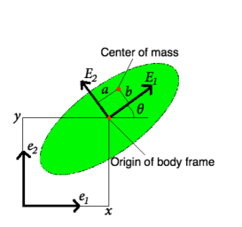
(a) Body frame is aligned with axes of symmetry of the body.

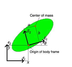
(b) Arbitrary position and orientation of the body frame.

Figure 1: Two different choices of the body frame for an elliptical two-dimensional rigid body. In both cases the origin of the body frame does not coincide with the center of mass.

We will often denote the above element in $g\in\operatorname{\operatorname{SE}}(2)$ by $g=(R_{\theta},{\bf x})$, where $R_{\theta}\in\operatorname{SO}(2)$ is the rotation matrix determined by the angle $\theta$. Let $(v_{1},v_{2})\in\mathbb{R}^{2}$ be the linear velocity of the origin of the body frame written in the body coordinates, and denote by $\omega=\dot{\theta}$ the body’s angular velocity. They define the element $\xi$ in the Lie algebra $\mathfrak{se}(2)$ given by

$$\xi=g^{-1}\dot{g}=\left(\begin{array}[]{ccc}0&-\omega&v_{1}\\ \omega&0&v_{2}\\ 0&0&0\end{array}\right)\in\mathfrak{se}(2).$$ (4.15)

Explicitly we have

$$\dot{\theta}=\omega,\qquad v_{1}=\dot{x}\cos\theta+\dot{y}\sin\theta,\quad v_{2}=-\dot{x}\sin\theta+\dot{y}\cos\theta.$$ (4.16)

For convenience, we will sometimes identify $\mathfrak{se}(2)$ with $\mathbb{R}^{3}$ as vector spaces, and denote $\xi\in\mathfrak{se}(2)$ as the column vector $(\omega,v_{1},v_{2})^{T}\in\mathbb{R}^{3}$. The Lie algebra commutator takes the form

$$\left[\,(\omega,v_{1},v_{2})\,,\,(\omega^{\prime},v_{1}^{\prime},v_{2}^{\prime})\,\right]_{\mathfrak{se}(2)}=(\,0\,,\,v_{2}\omega^{\prime}-\omega v_{2}^{\prime}\,,\,\omega v_{1}^{\prime}-v_{1}\omega^{\prime}\,).$$

For future reference, we give an explicit description of the dual space $\mathfrak{se}(2)^{\ast}$. Since $\mathfrak{se}(2)$ is isomorphic to $\mathbb{R}^{3}$ and using the Euclidian inner product, we have that $\mathfrak{se}(2)^{\ast}\cong\mathbb{R}^{3}$. A typical element $\mu$ is represented as a row vector $\mu=(k,p_{1},p_{2})$. The duality pairing between $\mu$ and an element $\xi=(\omega,v_{1},v_{2})^{T}$ of $\mathfrak{se}(2)$ is given by

$$\langle\mu,\xi\rangle=\mu\xi=k\omega+p_{1}v_{1}+p_{2}v_{2}.$$

The dual space $\mathfrak{se}(2)^{\ast}$ is equipped with the (minus) Lie-Poisson bracket, which is given by

$$\{F,K\}^{-}_{\mathfrak{se}(2)^{\ast}}(\mu)=-\left<\mu,\left[\frac{\delta F}{\delta\mu},\frac{\delta K}{\delta\mu}\right]\right>$$

for all functions $F,K$ on $\mathfrak{se}(2)^{\ast}$. In coordinates, we have

$$\{F,K\}^{-}_{\mathfrak{se}(2)^{\ast}}(\mu)=(\nabla_{\mu}F)^{T}\begin{pmatrix}0&-p_{2}&p_{1}\\ p_{2}&0&0\\ -p_{1}&0&0\end{pmatrix}(\nabla_{\mu}K),$$ (4.17)

where $\nabla_{\mu}F$ is the gradient of $F$ with respect to the variables $(k,p_{1},p_{2})=\mu$.

The fluid flow at a given instant.

Consider now the motion of the fluid that surrounds the body. Suppose that at a given instant the body occupies a region $\mathcal{B}\subset\mathbb{R}^{2}$. The flow is assumed to take place in the connected unbounded region $\mathcal{U}:=\mathbb{R}^{2}\setminus\mathcal{B}$ that is not occupied by the body. We assume that the flow is potential so the Eulerian velocity of the fluid ${\bf u}$ can be written as ${\bf u}=\nabla\Phi$ for a fluid potential $\Phi:\mathcal{U}\to\mathbb{R}$. Incompressibility of the fluid implies that $\Phi$ is harmonic,

$$\nabla^{2}\Phi=0\qquad\mbox{on}\qquad\mathcal{U}.$$

The boundary conditions for $\Phi$ come from the following considerations. On the one hand it is assumed that, up to a purely circulatory flow around the body, the motion of the fluid is solely due to the motion of the body. This assumption requires the fluid velocity $\nabla\Phi$ to vanish at infinity. Secondly, to avoid cavitation or penetration of the fluid into the body, we require the normal component of the fluid velocity at a material point $p$ on the boundary of $\mathcal{B}$ to agree with the normal component of the velocity of $p$. Suppose that the vector $(X,Y)\in\mathbb{R}^{2}$ gives body coordinates for $p$. The latter boundary condition is expressed as

$$\left.\frac{\partial\Phi}{\partial n}\right|_{p\in\partial\mathcal{B}}=(v_{1}-\omega Y)n_{1}+(v_{2}+\omega X)n_{2},$$

where ${\bf n}=(n_{1},n_{2})$ is the outward unit normal vector to $\mathcal{B}$ at $p$ written in body coordinates. These conditions determine the flow of the fluid up to a purely circulatory flow around the body that would persist if the body is brought to rest. The latter is specified by the value of the circulation $\kappa$ around the body as we now discuss.

The potential $\Phi$ that satisfies the above boundary value problem can be written in terms of the body’s velocities $\omega,v_{1},v_{2}$, in Kirchhoff form:

$$\Phi=\omega\chi+v_{1}\phi_{1}+v_{2}\phi_{2}+\phi_{0},$$ (4.18)

where $\phi_{i}$, $i=0,1,2$, and $\chi$ are harmonic functions on $\mathcal{U}$ whose gradients vanish at infinity and satisfy:

$$\left.\frac{\partial\phi_{i}}{\partial n}\right|_{\partial\mathcal{B}}=n_{i},\;i=1,2,\qquad\left.\frac{\partial\chi}{\partial n}\right|_{\partial\mathcal{B}}=Xn_{2}-Yn_{1},\qquad\left.\frac{\partial\phi_{0}}{\partial n}\right|_{\partial\mathcal{B}}=0.$$

The potential $\phi_{0}$ is multi-valued and defines the circulatory flow around the body. The circulation $\kappa$ of the fluid around the body satisfies

$$\kappa=\oint_{\partial\mathcal{B}}{\bf u}\cdot d{\mathbf{l}}=\oint_{\partial\mathcal{B}}\nabla\phi_{0}\cdot d{\mathbf{l}},$$ (4.19)

and remains constant during the motion.

The total kinetic energy of the fluid-body system.

Disregarding the circulatory motion, the kinetic energy of the fluid is given by

$$T_{\mathcal{F}}=\frac{\rho}{2}\int_{\mathcal{U}}||\nabla(\Phi-\phi_{0})||^{2}\,dA,$$

where $dA$ is the area element in $\mathbb{R}^{2}$ and $\rho$ is the (constant) fluid density. We have subtracted the circulatory part from the velocity potential, as it is known to give rise to an infinite contribution to the fluid kinetic energy and needs to be regularized away, as in [15, 18, 25].

By substituting (4.18) into the above, one can express $T_{\mathcal{F}}$ as the quadratic form

$$T_{\mathcal{F}}=\frac{1}{2}\left(\sum_{i,j=1}^{2}\mathcal{M}^{ij}_{\mathcal{F}}v_{i}v_{j}+2\sum_{i=1}^{2}\mathcal{K}^{i}_{\mathcal{F}}v_{i}\omega+\mathcal{I}_{\mathcal{F}}\omega^{2}\right),$$ (4.20)

where $\mathcal{M}_{\mathcal{F}}^{ij},\mathcal{K}_{\mathcal{F}}^{i}$, $i,j=1,2$, and $\mathcal{I}_{\mathcal{F}}$ are certain constants that only depend on the body shape. Explicitly one has (see [15] for details),

$$\begin{split}&\mathcal{M}^{ij}_{\mathcal{F}}=-\rho\int_{\partial\mathcal{B}}\phi_{i}\frac{\partial\phi_{j}}{\partial n}\,dl=-\rho\int_{\partial\mathcal{B}}\phi_{j}\frac{\partial\phi_{i}}{\partial n}\,dl,\;i,j=1,2,\qquad\mathcal{I}_{\mathcal{F}}=-\rho\int_{\partial\mathcal{B}}\chi\frac{\partial\chi}{\partial n}\,dl\\ &\mathcal{K}^{i}_{\mathcal{F}}=-\rho\int_{\partial\mathcal{B}}\phi_{i}\frac{\partial\chi}{\partial n}\,dl=-\rho\int_{\partial\mathcal{B}}\chi\frac{\partial\phi_{i}}{\partial n}\,dl,\;i=1,2.\end{split}$$

These constants are referred to as added masses and are conveniently written in $3\times 3$ matrix form to define the (symmetric) added inertia tensor:

$$\mathbb{I}_{\mathcal{F}}:=\left(\begin{array}[]{cc}\mathcal{I}_{\mathcal{F}}&\mathcal{K}_{\mathcal{F}}\\ \mathcal{K}_{\mathcal{F}}^{T}&\mathcal{M}_{\mathcal{F}}\end{array}\right),$$

that defines $T_{\mathcal{F}}$ as a quadratic form on $\mathfrak{se}(2)$.

On the other hand, the kinetic energy of the body is given by

$$T_{\mathcal{B}}=\frac{1}{2}\left((\mathcal{I}+m(a^{2}+b^{2}))\omega^{2}+mv_{1}^{2}+mv_{2}^{2}-mb\omega v_{1}+ma\omega v_{2}\right),$$

where $m$ is the total mass of the body and $\mathcal{I}$ is its moment of inertia of the body about its center of mass. We can write $T_{\mathcal{B}}$ as a quadratic form on $\mathfrak{se}(2)$ with matrix

$$\mathbb{I}_{\mathcal{B}}:=\left(\begin{array}[]{ccc}\mathcal{I}+m(a^{2}+b^{2})&-mb&ma\\ -mb&m&0\\ ma&0&m\end{array}\right).$$

We define $\mathbb{I}:=\mathbb{I}_{\mathcal{F}}+\mathbb{I}_{\mathcal{B}}$ as the total inertia tensor of the system. We consider it as an operator $\mathbb{I}:\mathfrak{se}(2)\to\mathfrak{se}(2)^{*}$ that satisfies that the left invariant Lagrangian defined at the identity by

$$L(\xi)=\frac{1}{2}\langle\mathbb{I}\xi,\xi\rangle,$$

is the total kinetic energy of the fluid-body system.

4.2 The Kirchhoff and Chaplygin-Lamb equations

The Kirchhoff equations.

The (reduced) equations of motion for the motion of a planar body in a potential flow, in the absence of circulation are the well-known Kirchhoff equations

$$\begin{split}\dot{k}&=v_{2}p_{1}-v_{1}p_{2},\\ \dot{p}_{1}&=\omega p_{2},\quad\quad\dot{p}_{2}=-\omega p_{1}.\end{split}$$ (4.21)

Here $k$ and $(p_{1},p_{2})$ are known as “impulsive pair” and “impulsive force” respectively. They are linearly related to the body’s velocities $\omega,v_{1},v_{2}$ via the total inertia tensor $\mathbb{I}$. The above equations are readily shown to be Hamiltonian with respect to the Lie-Poisson bracket (4.17) and the Hamiltonian function $H:\mathfrak{se}(2)^{*}\rightarrow\mathbb{R}$ given by

$$H(\mu)=\frac{1}{2}\mu\mathbb{I}^{-1}\mu^{T}.$$ (4.22)

The Chaplygin-Lamb equations.

In the presence of circulation, the Kirchhoff equations on $\mathfrak{se}(2)^{*}$ have to be modified to include the Kutta-Zhukowski force. This is a gyroscopic force, which is proportional to the circulation $\kappa$. In this case, the equations of motion are referred to as the Chaplygin-Lamb equations and they are given by

$$\begin{split}\dot{k}&=v_{2}p_{1}-v_{1}p_{2}-\rho(\alpha v_{1}+\beta v_{2}),\\ \dot{p}_{1}&=\omega p_{2}-\kappa\rho v_{2}+\rho\alpha\omega,\\ \dot{p}_{2}&=-\omega p_{1}+\kappa\rho v_{1}+\rho\beta\omega,\end{split}$$ (4.23)

where the constants $\alpha$ and $\beta$ are proportional to the circulation $\kappa$ and depend on the position and orientation of the body axes. They are explicitly given by:

$$\alpha=\oint_{\partial\mathcal{B}}X\nabla\phi_{0}\cdot\,d\mathbf{l},\qquad\beta=\oint_{\partial\mathcal{B}}Y\nabla\phi_{0}\cdot\,d\mathbf{l},$$ (4.24)

where, as before, $(X,Y)$ are body coordinates for material points in $\partial\mathcal{B}$. The Chaplygin-Lamb equations were first derived in [4, 15] and analyzed further in [2] (see also the references therein). In [29], the Chaplygin-Lamb equations were derived by considering the interaction between a rigid body and a potential flow with circulation, using techniques from symplectic reduction theory.

Remark 4.1.

One easily verifies that if the center of the body axes is displaced to the point with body coordinates $(r,s)$, so that the new body coordinates are $\tilde{X}=X-r,\;\tilde{Y}=Y-s$, then the circulation constants relative to the new coordinate axes take the form $\tilde{\alpha}=\alpha-r\kappa,\;\tilde{\beta}=\beta-s\kappa$. Thus, there is a unique choice of the body axes that makes these constants vanish. On the other hand, it is also often desirable to choose the body axes so that the total inertia tensor $\mathbb{I}$ is diagonal. For an asymmetric body, these two choices are in general incompatible, see e.g. [15]. $\diamond$

For our purposes, looking ahead to the introduction of the nonholonomic constraint, it is useful to consider equations (4.23) in their full generality where $\alpha,\,\beta\neq 0$, and $\mathbb{I}$ is not diagonal. This contrasts with the treatment in [29] where it is assumed that $\alpha=\beta=0$ and with [2] where the complementary assumption, namely that $\mathbb{I}$ is diagonal, is made.

It is shown in [29] that, if both circulation constants $\alpha$ and $\beta$ vanish, the Chaplygin-Lamb equations (4.23) can be interpreted as Lie-Poisson equations on the oscillator group that is a central extension of $\operatorname{SE}(2)$ by $\mathbb{R}$ and will be reviewed in Section 5. We will give a generalization of this result to the case in which $\alpha$ and $\beta$ are arbitrary. To do so, notice, by a direct calculation, that the equations (4.23) are Hamiltonian with respect to the usual Hamiltonian $H:\mathfrak{se}(2)^{*}\to\mathbb{R}$ given in (4.22) and with respect to the following non-canonical bracket of functions on $\mathfrak{se}(2)^{*}$:

$$\{F,K\}_{\kappa,\alpha,\beta}(\mu)=(\nabla_{\mu}F)^{T}\begin{pmatrix}0&-p_{2}&p_{1}\\ p_{2}&0&0\\ -p_{1}&0&0\end{pmatrix}(\nabla_{\mu}K)-\begin{pmatrix}\rho\kappa\\ -\rho\beta\\ \rho\alpha\end{pmatrix}\cdot\left((\nabla_{\mu}F)\times(\nabla_{\mu}K)\right).$$ (4.25)

Here “$\times$” denotes the standard vector product in $\mathbb{R}^{3}$, and, as before, $\nabla_{\mu}F$ is the gradient of $F$ with respect to the variables $(k,p_{1},p_{2})=\mu$. In fact we have:

Theorem 4.2.

The Chaplygin–Lamb equations (4.23) are of Lie-Poisson type on the dual Lie algebra $\widehat{\mathfrak{g}}^{*}=\mathfrak{se}(2)^{*}\times\mathbb{R}^{3}$ of a central extension of $\operatorname{\operatorname{SE}}(2)$ by $\mathbb{R}^{3}$.

The proof of this theorem is postponed to Section 5 where we introduce the appropriate central extension $\widehat{G}$ of $\operatorname{SE}(2)$. The explicit formula for the Lie-Poisson bracket on $\widehat{\mathfrak{g}}^{*}$ is given in Proposition 5.1. The non-canonical bracket (4.25) on $\mathfrak{se}(2)^{*}$ arises from the Lie-Poisson bracket on $\widehat{\mathfrak{g}}^{*}$ when one fixes the value $\boldsymbol{\sigma}=(\rho\kappa,-\rho\beta,\rho\alpha)\in\mathbb{R}^{3}$ as explained in Section 2, equations (2.5), (2.6).

4.3 The hydrodynamic Chaplygin sleigh with circulation

We now introduce the nonholonomic constraint. Recall that the classical Chaplygin sleigh problem (going back to 1911, [5]) describes the motion of a planar rigid body with a knife edge (a blade) sliding on a horizontal plane. The nonholonomic constraint forbids the motion in the direction perpendicular to the blade. In its hydrodynamic version, the body is surrounded by a potential fluid and the nonholonomic constraint models the effect of a very effective fin or keel, see [6].

With the notation of section 4.1, we let $\{{\bf E}_{1},{\bf E}_{2}\}$ be a body frame located at the contact point of the sleigh and the plane, and so that the ${\bf E}_{1}$-axis is aligned with the blade (see Figure 2).

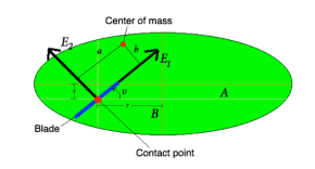
Figure 2: The hydrodynamic Chaplygin sleigh consists of a rigid body moving in a potential fluid equipped with a very effective fin or blade, which prevents motion in the direction lateral to the fin. The body frame $\{\mathbf{E}_{1},\mathbf{E}_{2}\}$ is taken so that $\mathbf{E}_{1}$ is aligned with the fin. The fin does not have to be aligned with any symmetry axes of the body, and we make no assumptions about the relative location of the center of mass, the geometric center of the body, and the contact point of the fin. We have depicted an elliptical body shape, but our results are valid for arbitrary convex shapes.

The resulting nonholonomic constraint is given by $v_{2}=0$, and is clearly left invariant under the action of $\operatorname{\operatorname{SE}}(2)$, as it is solely written in terms of the velocity of the body as seen in the body frame.

In the absence of constraints, the motion of the body is described by the Chaplygin–Lamb equations (4.23) that, as we have shown (Theorem 4.2), are Lie-Poisson equations on the dual Lie algebra of the central extension of $\operatorname{\operatorname{SE}}(2)$ by $\mathbb{R}^{3}$ and with respect to the kinetic energy Hamiltonian (4.22).

The reduced nonholonomic equations are thus of EPS type on $\widehat{\mathfrak{g}}^{*}=\mathfrak{se}(2)^{*}\times\mathbb{R}^{3}$. Note that the co-vector $(0,0,1)\in\mathfrak{g}^{*}$ annihilates all elements $\xi=(\omega,v_{1},v_{2})\in\mathfrak{se}(2)$ that satisfy the constraints. Thus, in agreement with the results of Theorem 4.2, by putting $\mu=(k,p_{1},p_{2})\in\mathfrak{se}(2)^{*}$ and $\sigma=(\rho\kappa,-\rho\beta,\rho\alpha)\in\mathbb{R}^{3}$, we get the following explicit expression for the reduced nonholonomic equations (3.12),

$$\begin{split}\dot{k}&=v_{2}p_{1}-v_{1}p_{2}-\rho(\alpha v_{1}+\beta v_{2}),\\ \dot{p}_{1}&=\omega p_{2}-\kappa\rho v_{2}+\rho\alpha\omega,\\ \dot{p}_{2}&=-\omega p_{1}+\kappa\rho v_{1}+\rho\beta\omega+\lambda,\end{split}$$ (4.26)

where the multiplier $\lambda$ is determined from the condition $v_{2}=0$.

Detailed equations of motion.

In the sequel we assume that the shape of the sleigh is arbitrary convex and that its center of mass does not necessarily coincide with the origin, which leads to the general total inertia tensor

$$\mathbb{I}=\left(\begin{array}[]{ccc}J&-L_{2}&L_{1}\\ -L_{2}&M&Z\\ L_{1}&Z&N\end{array}\right),$$

and with arbitrary circulation constants $\alpha,\,\beta$. The particular expressions for $\alpha,\beta$ and $\mathbb{I}$ in the case that the body is of elliptic shape are given in [7].

In accordance with (3.10), the multiplier $\lambda$ is given by:

$$\lambda=-\frac{1}{({\mathbb{I}^{-1}})_{33}}\left(\mathbb{I}^{-1}\left(\begin{array}[]{c}v_{2}p_{1}-v_{1}p_{2}-\rho(\alpha v_{1}+\beta v_{2})\\ \omega p_{2}-\kappa\rho v_{2}+\rho\alpha\omega\\ -\omega p_{1}+\kappa\rho v_{1}+\rho\beta\omega)\end{array}\right)\right)_{3},$$

where

$$\mathbb{I}^{-1}=\frac{1}{\mbox{det}(\mathbb{I})}\left(\begin{array}[]{ccc}MN-Z^{2}&ZL_{1}+NL_{2}&-ZL_{2}-ML_{1}\\ ZL_{1}+NL_{2}&JN-L_{1}^{2}&-L_{1}L_{2}-JZ\\ -ZL_{2}-ML_{1}&-L_{1}L_{2}-JZ&JM-L_{2}^{2}\end{array}\right).$$

A long but straightforward calculation shows that, by expressing $\omega,v_{1}$ and $v_{2}$ in terms of $k,p_{1},p_{2}$, substituting into (4.26), and enforcing the constraint $v_{2}=0$, one obtains:

$$\begin{split}\dot{\omega}&=\frac{1}{D}\left(L_{1}\omega+Zv_{1}+\rho\alpha\right)\left(L_{2}\omega-Mv_{1}\right),\\ \dot{v}_{1}&=\frac{1}{D}\left(L_{1}\omega+Zv_{1}+\rho\alpha\right)\left(J\omega-L_{2}v_{1}\right),\end{split}$$ (4.27)

where we set $D=\operatorname{det}(\mathbb{I})({\mathbb{I}^{-1}})_{33}=MJ-L_{2}^{2}$. Note that $D>0$ since $\mathbb{I}$ and $\mathbb{I}^{-1}$ are positive definite. Note as well that if $\alpha=0$ we recover the system with zero circulation treated in [6] so from now on we assume $\alpha\neq 0$.

The full motion of the sleigh on the plane is determined by the reconstruction equations which, in our case with $v_{2}=0$, reduce to

$$\dot{\theta}=\omega,\qquad\dot{x}=v_{1}\cos\theta,\qquad\dot{y}=v_{1}\sin\theta.$$

The reduced energy integral has

$$H=\frac{1}{2}\left(J\omega^{2}+Mv_{1}^{2}-2L_{2}\omega v_{1}\right),$$

and its level sets are ellipses on the $(\omega\,v_{1})$-plane.

As seen from the equations, the straight line $\ell=\{L_{1}\omega+Zv_{1}+\rho\alpha=0\}$ consists of equilibrium points for the system. Each of these equilibria corresponds to a uniform circular motion on the plane along a circumference of radius $\left|\frac{v_{1}}{\omega}\right|$.

Notice that if $Z=L_{1}=0$ the line $\ell$ of equilibra disappears. In fact, it is shown in [6] that in the absence of circulation the system possesses an invariant measure only for this specific value of the parameters. In view of Theorem 3.1 we conclude

Proposition 4.3.

The equations of motion (4.27) possess an invariant measure if and only if $Z=L_{1}=0$.

In this case we obtain simple harmonic motion on the reduced plane $\omega,v_{1}$. The reduced phase space in the case where $Z\neq 0$ and $L_{1}\neq 0$ is illustrated in Figure 3. As shown in [7], in this case there exists a positive value of the energy $h_{0}$ that divides periodic from heteroclinic orbits. The separatrix corresponding to $H=h_{0}$ is a homoclinic orbit.

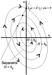
Figure 3: Reduced phase portrait. The line $\ell$ consists of equilibria that are either stable (filled dots) or unstable (empty dots). The trajectories are contained in the level surfaces of the Hamiltonian $H$ that are ellipses on the $v_{1}\;\omega$ plane.

For any value of the parameters the reduced system (4.27) can be checked to be Hamiltonian with respect to the following Poisson bracket of functions of $\omega,v_{1}$ that can be obtained using the results of [9]

$$\{F_{1},F_{2}\}:=-\frac{1}{D}\left(L_{1}\omega+Zv_{1}+\rho\alpha\right)\left(\frac{\partial F_{1}}{\partial\omega}\frac{\partial F_{2}}{\partial v_{1}}-\frac{\partial F_{1}}{\partial v_{1}}\frac{\partial F_{2}}{\partial\omega}\right).$$

The invariant symplectic leaves consist of the semi-planes separated by the equilibria line $\ell$ and the zero-dimensional leaves formed by the points on this line.

The integration of the reduced equations as well as a detailed study of the motion of the sleigh on the plane is given in [7].

5 Central extensions of the euclidean group $\operatorname{SE}(2)$

The purpose of this section is to explain in detail the central extension of $\operatorname{SE}(2)$ that encodes the effects of circulation in the Chaplygin-Lamb equations and appears in the statement of Theorem 4.2 and allows for the construction given in section 4.3.

5.1 The oscillator group

We start by defining the real valued $\operatorname{\operatorname{SE}}(2)$-two-cocycle $B_{1}:\operatorname{\operatorname{SE}}(2)\times\operatorname{\operatorname{SE}}(2)\to\mathbb{R}$ by

$$B_{1}((R_{\theta},{\bf x}),(R_{\theta^{\prime}},{\bf x}^{\prime}))=\frac{1}{2}{\bf x}\cdot\mathbb{J}R_{\theta}{\bf x}^{\prime},$$ (5.28)

where $\mathbb{J}$ is the $2\times 2$ symplectic matrix

$$\mathbb{J}=\left(\begin{array}[]{cc}0&1\\ -1&0\end{array}\right).$$

This cocycle differs from the one used in [29] by a multiplicative factor of $\frac{1}{2}$. On the Lie algebra level, we have by (2.3) that the infinitesimal cocycle $C_{1}:\mathfrak{se}(2)\times\mathfrak{se}(2)\to\mathbb{R}$ is given by

$$C_{1}\left((\omega,v_{1},v_{2}),(\omega^{\prime},v_{1}^{\prime},v_{2}^{\prime})\right)=v_{1}v_{2}^{\prime}-v_{2}v_{1}^{\prime}.$$

The central extension of $\operatorname{SE}(2)$ by $\mathbb{R}$ using the cocycle $B_{1}$ is referred to as the oscillator group [27], and will be denoted as $\mathrm{Osc}$. The Lie algebra $\mathfrak{osc}$ of the oscillator group is isomorphic to $\mathfrak{se}(2)\times\mathbb{R}$, with Lie bracket

$$\left[\,(\omega,v_{1},v_{2};z)\,,\,(\omega^{\prime},v_{1}^{\prime},v_{2}^{\prime};z^{\prime})\,\right]_{\mathfrak{osc}} =\left(\left[\,(\omega,v_{1},v_{2})\,,\,(\omega^{\prime},v_{1}^{\prime},v_{2}^{\prime})\,\right]_{\mathfrak{se}(2)}\,;\,C_{1}\left((\omega,v_{1},v_{2}),(\omega^{\prime},v_{1}^{\prime},v_{2}^{\prime})\right)\right)$$

$$=(\,0\,,\,v_{2}\omega^{\prime}-\omega v_{2}^{\prime}\,,\,\omega v_{1}^{\prime}-v_{1}\omega^{\prime}\,;\,v_{1}v_{2}^{\prime}-v_{2}v_{1}^{\prime}\,).$$

On the dual $\mathfrak{osc}^{\ast}\cong\mathfrak{se}(2)^{\ast}\times\mathbb{R}^{\ast}$, the (minus) Lie-Poisson bracket is given by (2.5), or explicitly by

$$\{F,K\}^{-}_{\mathfrak{osc}^{\ast}}(\mu,\sigma_{0})=\{F,K\}^{-}_{\mathfrak{se}(2)^{\ast}}(\mu)-\sigma_{0}C_{1}\left(\frac{\delta F}{\delta\mu},\frac{\delta K}{\delta\mu}\right),$$ (5.29)

for $(\mu,\sigma_{0})\in\mathfrak{se}(2)^{\ast}\times\mathbb{R}^{\ast}$. It is easy to see that this bracket coincides with the bracket (4.25) in the case where the circulation constants $\alpha$ and $\beta$ vanish, and where $\sigma_{0}$ plays the role of the circulation $\rho\kappa$. We conclude that, modulo the presence of non-zero circulation constants $\alpha$ and $\beta$, the effect of non-zero circulation can be described in terms of the geometry of the oscillator group, and more precisely the cocycle (5.28). This had already been established in [29].

In terms of Lie algebra cohomology, it is easy to show that $C_{1}$ is a closed two-cocycle which is not exact. Furthermore, as $H^{2}(\mathfrak{se}(2),\mathbb{R})$ is isomorphic to $\mathbb{R}$, we have that $C_{1}$ determines a generator of the second cohomology. Since isomorphy classes of central extensions are classified by the second Lie algebra cohomology, we may refer to the oscillator group as the central extension of $\operatorname{SE}(2)$ by $\mathbb{R}$.

5.2 A central extension of $\operatorname{\operatorname{SE}}(2)$ by $\mathbb{R}^{3}$.

We now describe the effect of nonzero $\alpha$ and $\beta$ in the Poisson bracket (4.25). To this end, we observe that the equations of motion (4.23) for nonzero $\alpha$ and $\beta$ can be obtained from the equations where $\alpha=\beta=0$ by making the substitution, or momentum shift,

$$p_{1}\leadsto p_{1}+\sigma_{1},\quad p_{2}\leadsto p_{2}+\sigma_{2},$$ (5.30)

where $\sigma_{1}=-\rho\beta$ and $\sigma_{2}=\rho\alpha$, while the angular momentum $k$ remains invariant. This observation seems natural in view of Remark 4.1.

The momentum shift (5.30) can be described in geometric terms as follows. Let $\mathcal{A}:\mathfrak{se}(2)\to\mathbb{R}^{3}$ be the linear map $\mathcal{A}(\omega,v_{1},v_{2})=(0,v_{1},v_{2})$. This map is a one-cocycle on $\mathfrak{se}(2)$ with values in $\mathbb{R}^{3}$ and its derivative is given by

$$\delta\mathcal{A}((\omega,v_{1},v_{2}),(\omega^{\prime},v_{1}^{\prime},v_{2}^{\prime}))=-\mathcal{A}([(\omega,v_{1},v_{2}),(\omega^{\prime},v_{1}^{\prime},v_{2}^{\prime})]_{\mathfrak{se}(2)})=(\,0\,,\,\omega v_{2}^{\prime}-v_{2}\omega^{\prime}\,,\,v_{1}\omega^{\prime}-\omega v_{1}^{\prime}\,).$$

Now, consider fixed values $\sigma_{1},\sigma_{2}\in\mathbb{R}$ and define the linear map $\mathcal{A}_{(\sigma_{1},\sigma_{2})}:\mathfrak{se}(2)\to\mathbb{R}$ given by

$$\mathcal{A}_{(\sigma_{1},\sigma_{2})}(\omega,v_{1},v_{2}):=\left<(0,\sigma_{1},\sigma_{2}),\mathcal{A}(\omega,v_{1},v_{2})\right>=\sigma_{1}v_{1}+\sigma_{2}v_{2}.$$

As $\mathcal{A}_{(\sigma_{1},\sigma_{2})}$ is an element of $\mathfrak{se}(2)^{\ast}$, we may write the momentum shift (5.30) more formally as the map $\Phi_{\mathcal{A}}:\mathfrak{se}(2)^{\ast}\to\mathfrak{se}(2)^{\ast}$ given by

$$\Phi_{\mathcal{A}}(\mu)=\mu-\mathcal{A}_{(\sigma_{1},\sigma_{2})},$$ (5.31)

for all $\mu\in\mathfrak{se}(2)^{\ast}$. The minus sign is due to the fact that this is the active version of the transformation (5.30): if we denote the new momenta of the system by $\bar{p}_{1},\bar{p}_{2}$, then the effect of performing the substitution (5.30) is that the old and the new momenta are related by $p_{1}=\bar{p}_{1}+\sigma_{1},p_{2}=\bar{p}_{2}+\sigma_{2}$, which is just (5.31).

As the dual of the Lie algebra of the oscillator group is just the Cartesian product $\mathfrak{se}(2)^{\ast}\times\mathbb{R}^{\ast}$, the map $\Phi_{\mathcal{A}}$ gives rise to a map $(\mu,\sigma_{0})\mapsto(\Phi_{\mathcal{A}}(\mu),\sigma_{0})$ on $\mathfrak{osc}^{\ast}$ which we denote by $\Phi_{\mathcal{A}}$ as well. We now investigate the behavior of the Poisson structure (5.29) under the map $\Phi_{\mathcal{A}}$. Since $\Phi_{\mathcal{A}}$ is a constant shift map, we have for arbitrary functions $F,K$ on $\mathfrak{osc}^{\ast}$ that

$$\frac{\delta(F\circ\Phi_{\mathcal{A}}^{-1})}{\delta\mu}=\frac{\delta F}{\delta\mu},$$

and similarly for $K$, so that $\{F\circ\Phi_{\mathcal{A}}^{-1},K\circ\Phi_{\mathcal{A}}^{-1}\}^{-}_{\mathfrak{osc}^{\ast}}(\mu,\sigma)=\{F,K\}^{-}_{\mathfrak{osc}^{\ast}}(\mu,\sigma)$. On the other hand,

$$\{F,K\}^{-}_{\mathfrak{osc}^{\ast}}(\Phi_{\mathcal{A}}^{-1}(\mu),\sigma) =\{F,K\}^{-}_{\mathfrak{se}(2)^{\ast}}(\Phi_{\mathcal{A}}^{-1}(\mu))-\sigma_{0}C_{1}\left(\frac{\delta F}{\delta\mu},\frac{\delta K}{\delta\mu}\right)$$

$$=\{F,K\}^{-}_{\mathfrak{se}(2)^{\ast}}(\mu)-\left<\mathcal{A}_{(\sigma_{1},\sigma_{2})},\left[\frac{\delta F}{\delta\mu},\frac{\delta K}{\delta\mu}\right]\right>-\sigma_{0}C_{1}\left(\frac{\delta F}{\delta\mu},\frac{\delta K}{\delta\mu}\right)$$

$$=\{F,K\}^{-}_{\mathfrak{se}(2)^{\ast}}(\mu)-\left(\sigma_{0}C_{1}-\delta\mathcal{A}_{(\sigma_{1},\sigma_{2})}\right)\left(\frac{\delta F}{\delta\mu},\frac{\delta K}{\delta\mu}\right),$$ (5.32)

so that $\Phi_{\mathcal{A}}$ takes the Lie-Poisson bracket on $\mathfrak{osc}^{\ast}$ into the bracket (5.32) modified by a cocycle. The cocycle $\sigma_{0}C_{1}-\delta\mathcal{A}_{(\sigma_{1},\sigma_{2})}$ can be made more explicit by noting that

$$(\sigma_{0}C_{1}-\delta\mathcal{A}_{(\sigma_{1},\sigma_{2})})((\omega,v_{1},v_{2}),(\omega^{\prime},v^{\prime}_{1},v^{\prime}_{2}))=\begin{bmatrix}\sigma_{0}\\ \sigma_{1}\\ \sigma_{2}\end{bmatrix}\cdot\begin{bmatrix}v_{1}v_{2}^{\prime}-v_{2}v_{1}^{\prime}\\ v_{2}\omega^{\prime}-\omega v_{2}^{\prime}\\ \omega v_{1}^{\prime}-v_{1}\omega^{\prime}\end{bmatrix}=\boldsymbol{\sigma}\cdot\left(\begin{bmatrix}\omega\\ v_{1}\\ v_{2}\end{bmatrix}\times\begin{bmatrix}\omega^{\prime}\\ v_{1}^{\prime}\\ v_{2}^{\prime}\end{bmatrix}\right),$$ (5.33)

where $\boldsymbol{\sigma}:=(\sigma_{0},\sigma_{1},\sigma_{2})$. Note that this is precisely the cocycle in the Poisson bracket (4.25) for the specific value of $\boldsymbol{\sigma}:=(\rho\kappa,-\rho\beta,\rho\alpha)$. We conclude that the effect of introducing nonzero $\sigma_{1},\sigma_{2}$ is to modify the Lie-Poisson bracket on $\mathfrak{osc}^{\ast}$ by a trivial $\mathbb{R}^{2}$-valued cocycle $-\delta\mathcal{A}_{(\sigma_{1},\sigma_{2})}$. We now let $C_{2}$ be equal to $-\delta\mathcal{A}$: this is an $\mathbb{R}^{3}$-valued cocycle on $\mathfrak{se}(2)$, which can be integrated to a group two-cocycle $B_{2}$ on $\operatorname{SE}(2)$, given by

$$B_{2}((R_{\theta},{\bf x}),(R_{\theta^{\prime}},{\bf x}^{\prime}))=(0,R_{\theta}{\bf x}^{\prime}-{\bf x}^{\prime}).$$ (5.34)

As we showed previously, we can describe the cocycle bracket (5.32) by considering the central extension of the oscillator group by the cocycle $B_{2}$ given in (5.34). This is equivalent to extending $\operatorname{SE}(2)$ by $\mathbb{R}^{3}$ using the combined cocycle $B:=(B_{1},B_{2}):\operatorname{SE}(2)\times\operatorname{SE}(2)\to\mathbb{R}^{3}$; the result is an extension $\widehat{G}$ which is isomorphic to $\operatorname{SE}(2)\times\mathbb{R}^{3}$ with multiplication

$$(R_{\theta},\mathbf{x};\mathbf{w})\cdot(R_{\theta^{\prime}},\mathbf{x}^{\prime};\mathbf{w}^{\prime})=(R_{\theta+\theta^{\prime}},\mathbf{x}+R_{\theta}\mathbf{x}^{\prime};\mathbf{w}+\mathbf{w}^{\prime}+B((R_{\theta},\mathbf{x}),(R_{\theta^{\prime}},\mathbf{x}^{\prime}))).$$

The infinitesimal cocycle $C:\mathfrak{se}(2)\times\mathfrak{se}(2)\to\mathbb{R}^{3}$ associated to $B$ is given by $C=(C_{1},C_{2})$, or

$$\begin{split}C((\omega,v_{1},v_{2}),(\omega^{\prime},v_{1}^{\prime},v_{2}^{\prime}))&=(v_{1}v_{2}^{\prime}-v_{2}v_{1}^{\prime},v_{2}\omega^{\prime}-\omega v_{2}^{\prime},\omega v_{1}^{\prime}-v_{1}\omega^{\prime})\\ &=(\omega,v_{1},v_{2})\times(\omega^{\prime},v_{1}^{\prime},v_{2}^{\prime}),\end{split}$$ (5.35)

which is precisely the cocycle appearing on the right-hand side of (5.33). The bracket on the algebra $\widehat{\mathfrak{g}}:=\mathrm{Lie}(\widehat{G})$ is then given by

$$\begin{split}[(\omega,v_{1},v_{2};{\bf z}),(\omega^{\prime},v_{1}^{\prime},v^{\prime}_{2};{\bf z}^{\prime})]_{\widehat{\mathfrak{g}}}&=\left(\left[\,(\omega,v_{1},v_{2})\,,\,(\omega^{\prime},v_{1}^{\prime},v_{2}^{\prime})\,\right]_{\mathfrak{se}(2)}\,;\,C\left((\omega,v_{1},v_{2}),(\omega^{\prime},v_{1}^{\prime},v_{2}^{\prime})\right)\right)\\ &=\left(\,0\,,\,v_{2}\omega^{\prime}-\omega v_{2}^{\prime}\,,\,\omega v_{1}^{\prime}-v_{1}\omega^{\prime}\,;\,v_{1}v_{2}^{\prime}-v_{2}v_{1}^{\prime},v_{2}\omega^{\prime}-\omega v_{2}^{\prime},\omega v_{1}^{\prime}-v_{1}\omega^{\prime}\,\right).\end{split}$$

The Lie-Poisson bracket on $\widehat{\mathfrak{g}}^{*}$.

We write explicitly the (minus) Lie-Poisson bracket on the dual Lie algebra $\widehat{\mathfrak{g}}^{*}$. Note first that as a vector space $\widehat{\mathfrak{g}}^{*}$ is just $\mathfrak{se}(2)^{*}\times\mathbb{R}^{3}$, so that an element $\nu$ of $\widehat{\mathfrak{g}}^{*}$ can be written as $\nu:=(\mu,\boldsymbol{\sigma})$ where $\mu\in\mathfrak{se}(2)^{*}$ and $\boldsymbol{\sigma}\in\mathbb{R}^{3}$. In view of (2.5) and (5.35) we obtain:

Proposition 5.1.

The (minus) Lie-Poisson bracket of functions $F,K\in C^{\infty}(\widehat{\mathfrak{g}}^{*})$ is given by

$$\{F,K\}^{-}_{\widehat{\mathfrak{g}}^{*}}(\mu,\boldsymbol{\sigma})=\{F,K\}^{-}_{{\mathfrak{se}(2)}^{*}}(\mu)-\boldsymbol{\sigma}\cdot\left(\frac{\delta F}{\delta\mu}\times\frac{\delta K}{\delta\mu}\right),$$

where we identify $\mathfrak{se}(2)$ with $\mathbb{R}^{3}$ in the usual way to make sense of the vector product of the functional derivatives.

In coordinates, the Poisson structure of the above proposition is

$$\{F,K\}^{-}_{\widehat{\mathfrak{g}}^{*}}(\mu,\boldsymbol{\sigma})=(\nabla_{(\mu,\boldsymbol{\sigma})}F)^{T}\,\left(\begin{array}[]{cccccc}0&-p_{2}-\sigma_{2}&p_{1}+\sigma_{1}&0&0&0\\ p_{2}+\sigma_{2}&0&-\sigma_{0}&0&0&0\\ -p_{1}-\sigma_{1}&\sigma_{0}&0&0&0&0\\ 0&0&0&0&0&0\\ 0&0&0&0&0&0\\ 0&0&0&0&0&0\end{array}\right)\,(\nabla_{(\mu,\boldsymbol{\sigma})}K),$$

where as usual $\mu=(k,p_{1},p_{2})\in\mathfrak{se}(2)^{*}$ and $\boldsymbol{\sigma}=(\sigma_{0},\sigma_{1},\sigma_{2})\in\mathbb{R}^{3}$.

Proof of Theorem 4.2.

Proof.

The reduced kinetic energy Hamiltonian $H(\mu)=\frac{1}{2}\mu\cdot\mathbb{I}^{-1}\mu$ on $\mathfrak{se}(2)^{*}$ defined in (4.22) is naturally interpreted as a Hamiltonian on $\widehat{\mathfrak{g}}^{*}$. The equations of motion for this Hamiltonian and the bracket $\{\cdot,\cdot\}^{-}_{\widehat{\mathfrak{g}}^{*}}$ are then given in coordinates by

$$\begin{split}\dot{k}&=-p_{2}v_{1}+p_{1}v_{2}-\sigma_{2}v_{1}+\sigma_{1}v_{2},\\ \dot{p}_{1}&=p_{2}\omega+\sigma_{2}\omega-\sigma_{0}v_{2},\\ \dot{p}_{2}&=-p_{1}\omega-\sigma_{1}\omega+\sigma_{0}v_{1},\\ \dot{\boldsymbol{\sigma}}&=0,\end{split}$$

that coincide with (4.23) if we put $\sigma_{0}=\rho\kappa,\;\sigma_{1}=-\rho\beta,\;\sigma_{2}=\rho\alpha$. ∎

Finally, we mention that the above equations possess the conserved quantity

$$\bar{F}(\mu,\boldsymbol{\sigma})=p_{1}^{2}+p_{2}^{2}+2\sigma_{0}k+2\sigma_{1}p_{1}+2\sigma_{2}p_{2},$$

which is a Casimir function of the bracket $\{\cdot,\cdot\}^{-}_{\widehat{\mathfrak{g}}^{*}}$. For a fixed value of $\boldsymbol{\sigma}$, the regular level sets of $\bar{F}$ define a symplectic foliation of $\mathfrak{se}(2)^{*}$. It is easily seen that the leaves of such foliation are paraboloids if $\sigma_{0}\neq 0$, and cylinders otherwise. The trajectories of the system are contained in the intersection of the level sets of $\bar{F}$ and $H$.

Future work

For the future, we intend to study the motion of the hydrodynamic Chaplygin sleigh coupled to point vortices in the fluid [20]. The equations of motion for interacting point vortices and rigid bodies (without nonholonomic constraints) were recently derived in [26, 3] and since then there have been significant efforts towards discerning integrability and chaoticity [22, 24] and towards uncovering the underlying geometry of these models [28]. We plan on coupling the nonholonomic Chaplygin sleigh with one or several point vortices in the flow, taking these models as our starting point. We hope to report with progress on these problems in the near future.

Acknowledgments.

We thank the GMC (Geometry, Mechanics and Control Network, project MTM2009-08166-E, Spain) for facilitating our collaboration during the events that it organizes. We thank Yuri Fedorov for his valuable suggestions and remarks. We are also thankful to Hassan Aref, Larry Bates, Paul Newton and J ‘ e drzej Śniatycki for useful and interesting discussions. JV is partially supported by the irses project geomech (nr. 246981) within the 7th European Community Framework Programme, and is on leave from a Postdoctoral Fellowship of the Research Foundation–Flanders (FWO-Vlaanderen). LGN thanks the hospitality of the Dipartimento de Matematica Pura e Applicata of University of Padova where part of this work was done.

References

• [1] A. Bloch. Nonholonomic mechanics and control, volume 24 of Interdisciplinary Applied Mathematics. Springer-Verlag, Berlin, 2003.
• [2] A. V. Borisov and I. S. Mamaev. On the motion of a heavy rigid body in an ideal fluid with circulation. Chaos, 16(1):013118, 7, 2006.
• [3] A. V. Borisov, I. S. Mamaev, and S. M. Ramodanov. Motion of a circular cylinder and $n$ point vortices in a perfect fluid. Regul. Chaotic Dyn., 8(4):449–462, 2003.
• [4] S. A. Chaplygin. On the effect of a plane-parallel air flow on a cylindrical wing moving in it. The Selected Works on Wing Theory of Sergei A. Chaplygin., pages 42–72, 1956. Translated from the 1933 Russian original by M. A. Garbell.
• [5] S. A. Chaplygin. On the theory of motion of nonholonomic systems. The reducing-multiplier theorem. Regul. Chaotic Dyn., 13(4):369–376, 2008. Translated from ıt Matematicheskiĭ sbornik (Russian) 28 (1911), no. 1 by A. V. Getling.
• [6] Y. N. Fedorov and L. C. García-Naranjo. The hydrodynamic Chaplygin sleigh. J. Phys. A, 43(43):434013, 18, 2010.
• [7] Y. N. Fedorov, L. C. García-Naranjo, and J. Vankerschaver. The motion of the 2D hydrodynamic Chaplygin sleigh in the presence of circulation. Accepted for publication in Disc. Cont. Dyn. Sys. A., 2012.
• [8] Y. N. Fedorov and V. V. Kozlov. Various aspects of $n$-dimensional rigid body dynamics. In Dynamical systems in classical mechanics, volume 168 of Amer. Math. Soc. Transl. Ser. 2, pages 141–171. Amer. Math. Soc., Providence, RI, 1995.
• [9] L. García-Naranjo. Reduction of almost Poisson brackets for nonholonomic systems on Lie groups. Regul. Chaotic Dyn., 12(4):365–388, 2007.
• [10] B. Jovanović. Non-holonomic geodesic flows on Lie groups and the integrable Suslov problem on ${\rm SO}(4)$. J. Phys. A, 31(5):1415–1422, 1998.
• [11] E. Kanso, J. E. Marsden, C. W. Rowley, and J. B. Melli-Huber. Locomotion of articulated bodies in a perfect fluid. J. Nonlinear Sci., 15(4):255–289, 2005.
• [12] S. D. Kelly and R. B. Hukkeri. Mechanics, Dynamics, and Control of a Single-Input Aquatic Vehicle With Variable Coefficient of Lift. IEEE Trans. on Robotics, 22(6):1254–1264, 2006.
• [13] B. Khesin and R. Wendt. The geometry of infinite-dimensional groups, volume 51 of Ergebnisse der Mathematik und ihrer Grenzgebiete. 3. Folge. A Series of Modern Surveys in Mathematics [Results in Mathematics and Related Areas. 3rd Series. A Series of Modern Surveys in Mathematics]. Springer-Verlag, Berlin, 2009.
• [14] V. V. Kozlov. Invariant measures of the Euler-Poincaré equations on Lie algebras. Funktsional. Anal. i Prilozhen., 22(1):69–70, 1988.
• [15] H. Lamb. Hydrodynamics. Dover Publications, 1945. Reprint of the 1932 Cambridge University Press edition.
• [16] P. Libermann and C.-M. Marle. Symplectic geometry and analytical mechanics, volume 35 of Mathematics and its Applications. D. Reidel Publishing Co., Dordrecht, 1987. Translated from the French by Bertram Eugene Schwarzbach.
• [17] J. E. Marsden, G. Misiołek, J.-P. Ortega, M. Perlmutter, and T. S. Ratiu. Hamiltonian reduction by stages, volume 1913 of Lecture Notes in Mathematics. Springer, Berlin, 2007.
• [18] L. Milne-Thomson. Theoretical hydrodynamics. London: MacMillan and Co. Ltd., fifth edition, revised and enlarged edition, 1968.
• [19] R. Montgomery. A tour of subriemannian geometries, their geodesics and applications, volume 91 of Mathematical Surveys and Monographs. American Mathematical Society, Providence, RI, 2002.
• [20] P. K. Newton. The $N$-vortex problem. Analytical techniques, volume 145 of Applied Mathematical Sciences. Springer-Verlag, New York, 2001.
• [21] S. P. Novikov. Variational methods and periodic solutions of equations of Kirchhoff type. II. Funktsional. Anal. i Prilozhen., 15(4):37–52, 96, 1981.
• [22] S. M. Ramodanov. Motion of a circular cylinder and a vortex in an ideal fluid. Regul. Chaotic Dyn., 6(1):33–38, 2001.
• [23] R. H. Rand and D. V. Ramani. Relaxing Nonholonomic Constraints. In A. Guran, editor, Proceedings of the First International Symposium on Impact and Friction of Fluids, Structures, and Intelligent Machines, pages 113–116, Singapore, 2000. World Scientific Publishing Co. Inc.
• [24] J. Roenby and H. Aref. Chaos in body-vortex interactions. Proc. R. Soc. Lond. Ser. A Math. Phys. Eng. Sci., 466(2119):1871–1891, 2010.
• [25] P. G. Saffman. Vortex dynamics. Cambridge Monographs on Mechanics and Applied Mathematics. Cambridge University Press, New York, 1992.
• [26] B. N. Shashikanth, J. E. Marsden, J. W. Burdick, and S. D. Kelly. The Hamiltonian structure of a two-dimensional rigid circular cylinder interacting dynamically with $N$ point vortices. Phys. Fluids, 14(3):1214–1227, 2002.
• [27] R. F. Streater. The representations of the oscillator group. Comm. Math. Phys., 4:217–236, 1967.
• [28] J. Vankerschaver, E. Kanso, and J. E. Marsden. The Geometry and Dynamics of Interacting Rigid Bodies and Point Vortices. J. Geom. Mech., 1(2):223–266, 2009.
• [29] J. Vankerschaver, E. Kanso, and J. E. Marsden. The dynamics of a rigid body in potential flow with circulation. Reg. Chaot. Dyn. (Special volume for the 60th birthday of V. V. Kozlov), 15(4-5):606–629, 2010.